| Issue |
A&A
Volume 501, Number 3, July III 2009
|
|
|---|---|---|
| Page(s) | 1013 - 1030 | |
| Section | Stellar structure and evolution | |
| DOI | https://doi.org/10.1051/0004-6361/200811073 | |
| Published online | 29 April 2009 | |
Variability of the transitional T Tauri star
T Chamaeleontis![[*]](/icons/foot_motif.png) ,
,
E. Schisano1,2 - E. Covino1 - J. M. Alcalá1 - M. Esposito3 - D. Gandolfi4 - E. W. Guenther4
1 -
INAF - Osservatorio Astronomico di Capodimonte,
via Moiariello 16,
80131 Napoli,
Italy
2 -
Università degli Studi di Napoli ``Federico II'',
Corso Umberto I,
80138 (NA)
Italy
3 -
Hamburger Sternwarte,
Gojenbergsweg 122,
21029 Hamburg,
Germany
4 -
Thüringer Landessternwarte Tautenburg,
Sternwarte 5,
07778 Tautenburg,
Germany
Received 2 October 2008 / Accepted 9 March 2009
Abstract
Context. It is known that for solar-mass stars planet formation begins in a circumstellar disc. The study of transitional objects exhibiting clear signs of evolution in their discs, such as the growth of dust particles and beginning of disc dispersal, is fundamental to understanding the processes governing dust-grain coagulation and the onset of planet formation.
Aims. We attempt to characterise the physical properties of T Chamaeleontis, a transitional T Tauri star showing UX Ori-type variability, and of its associated disc, and probe the possible effects of disc-clearing processes.
Methods. Different spectral diagnostics were examined, based on a rich collection of optical high- and low-resolution spectra. The cross-correlation technique was used to determine radial and projected rotational velocities, shape changes of photospheric lines were analysed via bisector-method applied to the cross-correlation profile, and the equivalent widths of both the Li I ![]() 6708 Å photospheric absorption and the most prominent emission lines (e.g., H
6708 Å photospheric absorption and the most prominent emission lines (e.g., H![]() ,
H
,
H![]() and [O I] 6300 Å) were measured. Variability in the main emission features was inspected by means of line-profile correlation matrices. Available optical and near-infrared photometry combined with infrared data from public catalogues was used to construct the spectral energy distribution (SED) and infer basic stellar and disc properties.
and [O I] 6300 Å) were measured. Variability in the main emission features was inspected by means of line-profile correlation matrices. Available optical and near-infrared photometry combined with infrared data from public catalogues was used to construct the spectral energy distribution (SED) and infer basic stellar and disc properties.
Results. Remarkable variability on timescale of days in the main emission lines, H![]() changing from pure emission to nearly photospheric absorption, is correlated with variations in visual extinction of over three magnitudes, while the photospheric absorption spectrum shows no major changes. The strength of emission in H
changing from pure emission to nearly photospheric absorption, is correlated with variations in visual extinction of over three magnitudes, while the photospheric absorption spectrum shows no major changes. The strength of emission in H![]() and H
and H![]() is highly variable and well correlated with that of the [O I] lines. The structure of the H
is highly variable and well correlated with that of the [O I] lines. The structure of the H![]() line-profile also varies on a daily time-span, while the absence of continuum veiling suggests very low or no mass accretion. Variations of up to nearly 10 km s-1 in the radial velocity of the star are measured on analogous timescales, but with no apparent periodicity. SED modelling confirms the existence of a gap in the disc.
line-profile also varies on a daily time-span, while the absence of continuum veiling suggests very low or no mass accretion. Variations of up to nearly 10 km s-1 in the radial velocity of the star are measured on analogous timescales, but with no apparent periodicity. SED modelling confirms the existence of a gap in the disc.
Conclusions. Variable circumstellar extinction is inferred to be responsible for the conspicuous variations observed in the stellar continuum flux and for concomitant changes in the emission features by contrast effect. Clumpy structures, incorporating large dust grains and orbiting the star within a few tenths of AU, obscure episodically the star and, eventually, part of the inner circumstellar zone, while the bulk of the hydrogen-line emitting-zone and outer low-density wind region traced by the [O I] remain unaffected. In agreement with this scenario, the detected radial velocity changes are also explainable in terms of clumpy material transiting and partially obscuring the star.
Key words: stars: variables: general - stars: pre-main sequence - stars: late-type - stars: individual: T Cha - stars: circumstellar matter - stars: planetary systems: protoplanetary discs
1 Introduction
T Tauri stars (TTS) are low-mass (
![]() )
pre-main sequence
(PMS) stars (Appenzeller & Mundt 1989).
They are commonly classified into two sub-groups, the classical TTS (cTTSs),
which are surrounded by an optically thick disc from which they accrete
material, and the weak TTS (wTTSs), presumably representing the final
stages of accretion and disc-clearing processes (Bertout et al. 2007).
Hence, the cTTS-wTTS dichotomy is ascribed to different physical
processes associated with the evolution of these young solar-type stars and
their circumstellar environment.
The equivalent width of the H
)
pre-main sequence
(PMS) stars (Appenzeller & Mundt 1989).
They are commonly classified into two sub-groups, the classical TTS (cTTSs),
which are surrounded by an optically thick disc from which they accrete
material, and the weak TTS (wTTSs), presumably representing the final
stages of accretion and disc-clearing processes (Bertout et al. 2007).
Hence, the cTTS-wTTS dichotomy is ascribed to different physical
processes associated with the evolution of these young solar-type stars and
their circumstellar environment.
The equivalent width of the H![]() emission is commonly used as an
empirical criterion to distinguish between cTTS and wTTS (White & Basri 2003).
However, due to possible variability, no clean distinction can be made between
the two subgroups based on the H
emission is commonly used as an
empirical criterion to distinguish between cTTS and wTTS (White & Basri 2003).
However, due to possible variability, no clean distinction can be made between
the two subgroups based on the H![]() emission alone.
emission alone.
Besides the traditional cTTS versus wTTS scheme, Herbst et al. (1994) introduced
an additional class, the early-type T Tauri stars (eTTSs), from
simple analysis of the photometric variability. ETTSs are earlier than K0 and
have large-amplitude irregular variations (up to ![]() 3 mag in V) with no
sign of continuum veiling. Within this class, those authors also included some
Herbig Ae/Be stars (HAEBEs) of the UX Ori type (Herbst et al. 1999). Studying
this kind of variability along with stellar mass, Bertout (2000)
concluded that T Tauri stars can display a similar phenomenology.
Well-studied cases such as RY Lup (Gahm et al. 1989) and AA Tau (Bouvier et al. 2003)
support this hypothesis.
3 mag in V) with no
sign of continuum veiling. Within this class, those authors also included some
Herbig Ae/Be stars (HAEBEs) of the UX Ori type (Herbst et al. 1999). Studying
this kind of variability along with stellar mass, Bertout (2000)
concluded that T Tauri stars can display a similar phenomenology.
Well-studied cases such as RY Lup (Gahm et al. 1989) and AA Tau (Bouvier et al. 2003)
support this hypothesis.
How can all these observations be interpreted coherently in a scenario of star and circumstellar environment evolution is still questioned. Grinin (1988) modelled this kind of variability with dusty clumps in Keplerian orbits that temporarily obscure the central star. The rapid temporal evolution of such events indicates that the dust clouds usually appear in the disc close to the dust sublimation radius, probably in the inner rim region (Dullemond et al. 2003; Natta et al. 2001). This model implies a high inclination angle, while imaging and near-infrared interferometry of some of those stars are inconsistent with it (see the review by Millan-Gabet et al. 2007, and references therein). Another scenario was proposed by Vinkovic & Jurkic (2007), in which a dusty outflow creates a halo in the inner-disc region, where clumps of dust occasionally intercept the line of sight and mask the stellar photosphere.
T Tauri discs evolve on a timescale of a few million years and the
circumstellar raw material from which planets are constructed is affected
different processes. In the inner part of the disc (![]() 10 AU),
the gas is accreted onto the star or expelled by bipolar jets,
while the outer part of the disc may be dissipated by photoevaporation
(Clarke et al. 2001; Alexander & Armitage 2007).
On the other hand, dust grains settle in the midplane, grow in size, and
form planetesimals (Dullemond & Dominik 2005; Sicilia-Aguilar et al. 2007).
As the disc becomes progressively optically thin, solid particles migrate
inward or outward, depending on their size, due to the combined action of
different perturbing forces (photophoresis, gravity, radiation pressure, and gas drag),
until they reach a stability distance from the star (Hermann et al. 2007).
It remains unclear how planetesimals are formed in circumstellar discs and whether
the hypothetical
dusty clumps in highly variable TTS are related or not to the evolution of
circumstellar dust until the formation of planetesimals.
Detailed studies of the observed properties of objects with intermediate
characteristics, in-between those of cTTS and wTTS, are expected to provide
key constraints on star and planet formation scenarios.
10 AU),
the gas is accreted onto the star or expelled by bipolar jets,
while the outer part of the disc may be dissipated by photoevaporation
(Clarke et al. 2001; Alexander & Armitage 2007).
On the other hand, dust grains settle in the midplane, grow in size, and
form planetesimals (Dullemond & Dominik 2005; Sicilia-Aguilar et al. 2007).
As the disc becomes progressively optically thin, solid particles migrate
inward or outward, depending on their size, due to the combined action of
different perturbing forces (photophoresis, gravity, radiation pressure, and gas drag),
until they reach a stability distance from the star (Hermann et al. 2007).
It remains unclear how planetesimals are formed in circumstellar discs and whether
the hypothetical
dusty clumps in highly variable TTS are related or not to the evolution of
circumstellar dust until the formation of planetesimals.
Detailed studies of the observed properties of objects with intermediate
characteristics, in-between those of cTTS and wTTS, are expected to provide
key constraints on star and planet formation scenarios.
Observations in the infrared (IR) with the Spitzer satellite have provided a
wealth of information for interpretating the spectral energy distribution (SED)
of young stars (see Lada et al. 2006; Cieza et al. 2007; Evans et al. 2008, and references therein),
allowing the development of new classification schemes and scenarios of disc evolution
(e.g., Merín et al. 2008; Cieza 2008). In particular, young stellar objects with
no IR excess shortward of 10 ![]() m, but with significant excess emission
at wavelengths longer than
m, but with significant excess emission
at wavelengths longer than ![]() 24
24 ![]() m, are interpreted as being in an
evolutionary phase of disc clearing and are hence classified as transitional
objects (Najita et al. 2007; Furlan et al. 2006). Evidence for gaps in the
disc of transitional objects have also been reported (Espaillat et al. 2008; Brown et al. 2007).
In one of these, LkCa 15, the most likely mechanism for gap-opening in the disc
seems to be planet formation (Espaillat et al. 2008). Disc clearing may also
be due to the presence of a companion, as in the case of CoKu Tau/4
(Ireland & Kraus 2008).
m, are interpreted as being in an
evolutionary phase of disc clearing and are hence classified as transitional
objects (Najita et al. 2007; Furlan et al. 2006). Evidence for gaps in the
disc of transitional objects have also been reported (Espaillat et al. 2008; Brown et al. 2007).
In one of these, LkCa 15, the most likely mechanism for gap-opening in the disc
seems to be planet formation (Espaillat et al. 2008). Disc clearing may also
be due to the presence of a companion, as in the case of CoKu Tau/4
(Ireland & Kraus 2008).
Here we present a synoptic study of the spectroscopic variability of T Chamaeleontis (hereafter T Cha), a transitional T Tauri star (Brown et al. 2007) displaying a UX Ori-like behaviour. T Cha was observed in the course of a project aiming to reveal and monitor young spectroscopic binary systems (Esposito et al. 2006; Guenther et al. 2007).
The scheme of the paper is the following. In Sect. 2 we summarise
the main observed properties of T Cha as known from previous studies.
In Sect. 3 we present the observations and data reduction,
while in Sect. 4 we describe the radial velocity and
![]() determinations. In Sects. 5 and 6, we report the
analysis performed on the spectrum of the object, focusing on the non-photospheric
contribution and, in particular, on the variability of the most prominent emission
features (e.g., H
determinations. In Sects. 5 and 6, we report the
analysis performed on the spectrum of the object, focusing on the non-photospheric
contribution and, in particular, on the variability of the most prominent emission
features (e.g., H![]() ,
H
,
H![]() ,
and the [O I] 6300 Å lines).
In Sect. 8 we analyse the spectral energy distribution of T Cha, while
in Sect. 9 we discuss the results and present our interpretation of the object.
,
and the [O I] 6300 Å lines).
In Sect. 8 we analyse the spectral energy distribution of T Cha, while
in Sect. 9 we discuss the results and present our interpretation of the object.
2 Observed properties of T Cha
T Cha shows strong photometric variability (up to 3 mag in the V-band)
mainly characterised by erratic changes (Covino et al. 1992; Mauder & Sosna 1975; Hoffmeister 1958), and by a UX Ori-like behaviour (i.e., the star becomes redder as it fades),
with a tight correlation between brightness and colour (Covino et al. 1996; Alcalá et al. 1993).
A periodicity of 3
![]() 2 was found by Mauder & Sosna (1975).
Spectroscopic variability in the most prominent emission lines was reported by
Gregorio-Hetem et al. (1992) and Alcalá et al. (1993).
2 was found by Mauder & Sosna (1975).
Spectroscopic variability in the most prominent emission lines was reported by
Gregorio-Hetem et al. (1992) and Alcalá et al. (1993).
The PMS nature of T Cha was established by Alcalá et al. (1993) on the basis of the lithium
criterion combined with the H![]() emission strength and the presence of strong IR excess
emission, while the spectral type G8 V (Alcalá et al. 1993) is earlier than that of
a typical T Tauri star.
From the strength of the H
emission strength and the presence of strong IR excess
emission, while the spectral type G8 V (Alcalá et al. 1993) is earlier than that of
a typical T Tauri star.
From the strength of the H![]() emission in former spectra, T Cha had been initially
regarded as a wTTS (Alcalá et al. 1993), but later this classification turned out to be inconsistent
with the strong variability of the star (Gras-Velazques & Ray 2005; Alcalá et al. 1995; Geers et al. 2006).
Moreover, besides the IR excess indicating the presence of circumstellar material,
the object occasionally exhibits forbidden neutral oxygen lines that are not seen
in wTTS spectra.
Brown et al. (2007) modelled the SED and interpreted it in terms of a transitional disc.
emission in former spectra, T Cha had been initially
regarded as a wTTS (Alcalá et al. 1993), but later this classification turned out to be inconsistent
with the strong variability of the star (Gras-Velazques & Ray 2005; Alcalá et al. 1995; Geers et al. 2006).
Moreover, besides the IR excess indicating the presence of circumstellar material,
the object occasionally exhibits forbidden neutral oxygen lines that are not seen
in wTTS spectra.
Brown et al. (2007) modelled the SED and interpreted it in terms of a transitional disc.
T Cha is located near the edge of the small cloud G300.2-16.9, also known as the Blue Cloud, in the direction of the Chamaeleon dark cloud complex (Nehme et al. 2008). In the Hipparcos Catalogue, a distance of 66 +19-12 pc is reported, although the error in the parallax is probably far higher because of the strong variability of the star (reported to vary between 10.4 and 13.4 mag in the HP-band during the period of observation). More reliable estimates of the distance were obtained from proper motion studies by Frink et al. (1998) and by Terranegra et al. (1999), suggesting that T Cha is part of an association of stars at nearly 100 pc. Here we adopt the latter value.
3 Observations and data reduction
3.1 High-resolution spectroscopy
Data were acquired at the ESO-La Silla Observatory using the echelle spectrograph FEROS
(Fiber-fed Extended Range Optical Spectrograph), first installed at the 1.5 m and, since
October 2002, then mounted at the 2.2 m telescope.
The high resolving power (
![]() )
and the wide useful spectral range (
3600-9200 Å)
make FEROS particularly suitable for radial-velocity (RV) monitoring and spectral-line
variability studies.
FEROS was operated in the
)
and the wide useful spectral range (
3600-9200 Å)
make FEROS particularly suitable for radial-velocity (RV) monitoring and spectral-line
variability studies.
FEROS was operated in the
![]() configuration, in which a sky
spectrum is acquired simultaneously with the object through an adjacent fiber.
configuration, in which a sky
spectrum is acquired simultaneously with the object through an adjacent fiber.
From 1999 to 2006, we obtained a total of 50 FEROS spectra with quite different signal-to-noise ratios (S/N), due not only to the change of telescope or different observing conditions but also to the strong variability of the star. The spectra were acquired within the framework of a project on young spectroscopic binary systems. For that reason, the time coverage of our data is rather uneven, with some spectra acquired on daily temporal base and others separated by several months.
The data reduction was performed using the specific FEROS Data Reduction Software (DRS)
implemented in the ESO-MIDAS![]() environment.
The reduction steps were the following:
bias subtraction and bad-column masking; definition of the echelle orders on
flat-field frames; subtraction of the background diffuse light; order extraction;
order by order flat-fielding; determination of wavelength-dispersion solution
by means of ThAr calibration-lamp exposures; rebinning to a linear wavelength-scale
(
environment.
The reduction steps were the following:
bias subtraction and bad-column masking; definition of the echelle orders on
flat-field frames; subtraction of the background diffuse light; order extraction;
order by order flat-fielding; determination of wavelength-dispersion solution
by means of ThAr calibration-lamp exposures; rebinning to a linear wavelength-scale
(
![]() Å) with barycentric correction; and merging of the echelle orders.
All the spectra were then normalized to the continuum.
Å) with barycentric correction; and merging of the echelle orders.
All the spectra were then normalized to the continuum.
More details about the data reduction procedure and technical specifications
of the instrument can be found at the FEROS Web
site![]() .
We emphasise that the high stability of the instrument allows an internal accuracy
in the wavelength calibration of approximately 200 m s-1 (average residual
.
We emphasise that the high stability of the instrument allows an internal accuracy
in the wavelength calibration of approximately 200 m s-1 (average residual
![]() Å).
A log of the FEROS observations is provided in Table 1.
Å).
A log of the FEROS observations is provided in Table 1.
Apart from the FEROS data, we also report measurements from a previous set of six high-resolution CASPEC spectra obtained simultaneously with optical broad-band photometry on two consecutive nights, 1994 January 31 and February 1 (Covino et al. 1996). Details about the instrumental set-up and data reduction can be found in Covino et al. (1997).
3.2 Low-resolution spectroscopy
In addition to the high-resolution spectroscopy, we include unpublished
low-resolution (
![]() )
spectra gathered during various observing runs
conducted between 1993 and 1995 using the Boller & Chivens spectrograph at the
ESO 1.5 m telescope at La Silla, Chile.
The reduction of these data was performed as described in Alcalá et al. (1995).
We recall that these spectra were calibrated in relative fluxes using a standard star.
)
spectra gathered during various observing runs
conducted between 1993 and 1995 using the Boller & Chivens spectrograph at the
ESO 1.5 m telescope at La Silla, Chile.
The reduction of these data was performed as described in Alcalá et al. (1995).
We recall that these spectra were calibrated in relative fluxes using a standard star.
4 Cross-correlation function analysis
![\begin{figure}
\par\includegraphics[width=8cm,clip]{1073f1.ps}
\end{figure}](/articles/aa/full_html/2009/27/aa11073-08/img26.png) |
Figure 1:
Changes in the CCF in the period 19-23 May 2000, in two different
wavelength ranges. The different colours refer to the following dates:
19 May (
|
| Open with DEXTER | |
![\begin{figure}
\par\includegraphics[width=8cm,clip]{1073f2.ps}
\end{figure}](/articles/aa/full_html/2009/27/aa11073-08/img27.png) |
Figure 2:
CCF peaks between 16 and 22 May 1999 ( upper panel).
Velocity is relative to the template star.
The different colours refer to the following dates: 16 May (
|
| Open with DEXTER | |
4.1 Radial velocity determinations
We used the cross-correlation technique to determine the radial velocity of T Cha from the FEROS spectra. As a template, we chose a spectrum of the G8.5 V star HD 152 391 (RV = 44.8 km s-1 andWe followed the prescription by Esposito et al. (2006), i.e., a Gaussian was fitted to the peak of the cross-correlation function (CCF), computed in six distinct spectral ranges. In some cases, the Gaussian fit failed, and in such cases we calculated the moments of the CCF profile and took the first-order moment as an RV estimator. In the end, we adopted as RV value and associated error, the average of the RV determined in the different ranges and their rms dispersion, respectively. All RV measurements are reported in Table 1. The RV values vary with time ranging between 6 and 30 km s-1. A period search was performed on these data, but no clear indication of periodicity was found.
4.2 CCF bisector analysis
The Gaussian fit may sometimes appear inadequate due to asymmetries in the CCF peak. Asymmetries in stellar absorption lines can arise for several reasons and may be conveniently represented by line bisectors (Gray 2005). In some cases, variations in the bisector shape may arise due to photospheric spots crossing the stellar disc as the star rotates, whereas uncorrelated variations in both bisector position and shape may indicate an unresolved spectroscopic system (Dall et al. 2006; Santos et al. 2002).From the correlation between RV changes and bisector orientation, Queloz et al. (2001), in the case of HD 166 435, stated that the periodicity in their RV data was not due to an unseen secondary object orbiting the star, but to stellar activity. We adopted the same tool to verify whether RV shifts measured by a Gaussian fit are purely due to changes in the CCF peak shape, or reflect true changes in the radial velocity of the star. An example of the variability of the CCF peak (and corresponding bisector) of T Cha on daily timescales is shown in Figs. 1 and 2. For each of the six spectral ranges considered in Sect. 4.1, we divided the corresponding CCF bisector into two intervals as in Queloz et al. (2001): an upper part, where the strongest changes occur, and a lower one, where the bisector position appears more stable (see in Fig. 2). The RV difference between the top and bottom bisector's mean velocities yields information about the bisector orientation. This quantity, called ``bisector velocity span'' (Queloz et al. 2001; Dall et al. 2006; Toner & Gray 1988), is a good measure of the changes in bisector orientation, and hence of the asymmetry of the peak. The variations in the central part of the CCF, which reflect the higher stability of the wings compared to the peak can be easily discerned.
The comparison between the RV values obtained from a Gaussian-fit and by a bisector analysis
is shown in Fig. 3.
The left panel shows how the RV values from a Gaussian-fit are well correlated with the
bisector velocity span![]() .
The Gaussian function reproduces well only one of the two sides of an asymmetric CCF peak,
leading to a systematic shift in the measured RV.
On the other hand, the bisector values, at the bottom part of the profile, versus the
bisector span show a weaker correlation than the Gaussian-fit values
(Fig. 3 right panel).
.
The Gaussian function reproduces well only one of the two sides of an asymmetric CCF peak,
leading to a systematic shift in the measured RV.
On the other hand, the bisector values, at the bottom part of the profile, versus the
bisector span show a weaker correlation than the Gaussian-fit values
(Fig. 3 right panel).
The RV determinations derived from the bisector method, although of lower amplitude than the values derived from the Gaussian-fit method, confirm that RV is indeed variable, considering the average uncertainty of 1.7 km s-1. We performed Fourier analysis, using the formulation of the periodogram given by Scargle (1982), to search for possible periodicities in the radial velocity data, although no clear values were identified. This might in part be due to the extremely uneven temporal sampling. We had only one relatively long run of six consecutive nights, but when analysing this run alone, no hint of periodicity was found on a timescale of a few days.
Although the presence of blended spectroscopic components cannot be excluded, the lack of a clear periodicity prevents us from drawing firm conclusions about the possible binarity or multiple-nature of T Cha. As in Queloz et al. (2001), the correlations between the RV values from the Gaussian-fit method and the ``velocity span'' indicate as most plausible explanation the presence of inhomogeneities of variable extent moving across the photospheric disc, either intrinsic to the star (e.g., cool spots), or external to it (e.g., clustered orbiting material). Hence, in the following, T Cha will be treated as a single star. For the purposes of photospheric spectrum subtraction (see Sect. 5.2), we used the bottom bisector's mean RV value.
![\begin{figure}
\par\includegraphics[width=8.cm,height=7.5cm,angle=-90,clip]{1073...
...ncludegraphics[width=8.cm,height=7.5cm,angle=-90,clip]{1073f3b.ps}
\end{figure}](/articles/aa/full_html/2009/27/aa11073-08/img29.png) |
Figure 3: The radial velocity measurements from Gaussian-fit method versus the ``bisector velocity span'' (i.e. the difference between the upper and bottom bisector mean velocities) are plotted in the left panel. The right panel shows, instead, the mean radial velocity of the CCF bisector bottom versus the ``bisector velocity span''. |
| Open with DEXTER | |
4.3 Projected rotational velocity
We evaluated the projected rotational velocity, ![]() ,
of T Cha by measuring
the full width at half maximum (FWHM) of the CCF peak for the spectra with higher signal-to-noise ratio.
We first established a relation between the FWHM and
,
of T Cha by measuring
the full width at half maximum (FWHM) of the CCF peak for the spectra with higher signal-to-noise ratio.
We first established a relation between the FWHM and ![]() ,
as described in Covino et al. (1997),
using the template spectrum of HD 152391 broadened artificially by various
,
as described in Covino et al. (1997),
using the template spectrum of HD 152391 broadened artificially by various ![]() values.
The
values.
The ![]() value determined in this way was
value determined in this way was ![]() km s-1.
The same measurement was repeated on an average spectrum obtained by combining a total of
34 spectra with
km s-1.
The same measurement was repeated on an average spectrum obtained by combining a total of
34 spectra with ![]() around 6000 Å.
The
around 6000 Å.
The ![]() determined in the average spectrum is consistent with the previous value.
However, when extending the measurements to all spectra, we identified a few with
narrower spectral lines, yielding a
determined in the average spectrum is consistent with the previous value.
However, when extending the measurements to all spectra, we identified a few with
narrower spectral lines, yielding a ![]() of nearly 30 km s-1.
Hence, we checked the
of nearly 30 km s-1.
Hence, we checked the ![]() determinations by directly fitting each spectrum with
an artificially broadened template, which confirmed that some spectra had
smaller line widths.
determinations by directly fitting each spectrum with
an artificially broadened template, which confirmed that some spectra had
smaller line widths.
In Fig. 4, we report the ![]() values obtained from CCF Gaussian-fit FWHM calibration versus
the width at half maximum of the CCF peak measured directly.
In this case, it is obvious that the width of the lines does not provide a reliable measure
of the rotational velocity.
A variable line-width is indicative of either blended spectroscopic components
or the presence of inhomogeneities moving across the stellar disc that alter the shape of
photospheric lines.
However, no correlation is found between the RV (either from a Gaussian-fit or bisector method)
and the
values obtained from CCF Gaussian-fit FWHM calibration versus
the width at half maximum of the CCF peak measured directly.
In this case, it is obvious that the width of the lines does not provide a reliable measure
of the rotational velocity.
A variable line-width is indicative of either blended spectroscopic components
or the presence of inhomogeneities moving across the stellar disc that alter the shape of
photospheric lines.
However, no correlation is found between the RV (either from a Gaussian-fit or bisector method)
and the ![]() measurements.
measurements.
From a periodogram analysis based on data points from the spectra of higher signal-to-noise ratio, we found a peak at about 0.25 cycles day-1, or a period close to 4 days. This period does not differ dramatically from that found by Mauder & Sosna (1975) and might reflect a rotational modulation induced by photospheric spots or other types of inhomogeneities transiting over the stellar disc.
5 The spectrum of T Cha
5.1 Photospheric spectrum and lithium abundance
The spectrum of T Cha is that of a G8 V star with strong absorption in the
Li I resonance line at ![]() 6708 Å and a few emission lines
typical of TTS. The spectral type does not change from one spectrum to the other,
as also demonstrated in Sect. 7.
Figure 5 shows the good match between the photospheric spectrum of T Cha
and that of the template. The equivalent width (EW) of the lithium line was measured
in each spectrum of our FEROS data-set. The measurements were found to be internally
consistent, within the errors, yielding a mean value of
6708 Å and a few emission lines
typical of TTS. The spectral type does not change from one spectrum to the other,
as also demonstrated in Sect. 7.
Figure 5 shows the good match between the photospheric spectrum of T Cha
and that of the template. The equivalent width (EW) of the lithium line was measured
in each spectrum of our FEROS data-set. The measurements were found to be internally
consistent, within the errors, yielding a mean value of
![]() mÅ.
Using the calibration of Pavlenko & Magazzú (1996) and adopting the temperature of
5000 K, we derived a lithium abundance compatible with the cosmic value
(
mÅ.
Using the calibration of Pavlenko & Magazzú (1996) and adopting the temperature of
5000 K, we derived a lithium abundance compatible with the cosmic value
(
![]() ), with an uncertainty of 0.2 dex.
It is important to recall that this determination is strictly dependent on
the effective temperature. At a temperature of 5500 K, as adopted by
Kenyon & Hartmann (1995) for a G8 V star, the abundance would increase to 3.6 dex,
implying some lithium enrichment with respect to the interstellar value.
), with an uncertainty of 0.2 dex.
It is important to recall that this determination is strictly dependent on
the effective temperature. At a temperature of 5500 K, as adopted by
Kenyon & Hartmann (1995) for a G8 V star, the abundance would increase to 3.6 dex,
implying some lithium enrichment with respect to the interstellar value.
![\begin{figure}
\par\resizebox{9cm}{!}{\rotatebox[]{-90}{\includegraphics[width=7cm, height=8cm,trim = 10mm 10mm 0mm 0mm, clip]{1073f4.ps}}}
\end{figure}](/articles/aa/full_html/2009/27/aa11073-08/img34.png) |
Figure 4: Projected rotational velocity from CCF Gaussian-fit calibration versus FWHM of the CCF peak. Only the data of the highest S/N are considered here. |
| Open with DEXTER | |
5.2 Photospheric spectrum subtraction
One of the main goals of this work was to analyse the variability in the emission lines and hence probe the circumstellar environment of T Cha. For this purpose, it is useful to remove the photospheric contribution. We subtracted the photospheric-line spectrum from the FEROS spectra of T Cha using the same template spectrum of HD 152 391 used in the cross-correlation analysis presented in Sect. 4.
All spectra were rebinned to the rest-wavelength frame to take account of
their different RV shifts, derived from the CCF analysis described in Sect. 4.1.
The template spectrum was broadened artificially by the ![]() value of
37 km s-1 and then subtracted from each of the T Cha spectra.
We assumed that the photospheric spectrum of a TTS resembles that
of a main-sequence star of the same spectral type. The photospheric subtraction
method also allows us to verify the possible presence of ``veiling''. No sign
of continuum excess emission was found in T Cha (see Fig. 20),
confirming the absence of UV-excess in the broad-band photometry
(see Sect. 8 and Covino et al. 1996).
value of
37 km s-1 and then subtracted from each of the T Cha spectra.
We assumed that the photospheric spectrum of a TTS resembles that
of a main-sequence star of the same spectral type. The photospheric subtraction
method also allows us to verify the possible presence of ``veiling''. No sign
of continuum excess emission was found in T Cha (see Fig. 20),
confirming the absence of UV-excess in the broad-band photometry
(see Sect. 8 and Covino et al. 1996).
Examples of the residual profiles of the main emission lines at different dates are shown in Fig. 6.
Some lines show absorption components shifted toward shorter and/or longer wavelengths.
The H![]() line is the most variable in both intensity and shape.
The residuals of the Na I D lines show either redshifted or blue-shifted absorption
components (that are easily distinguishable from the sharp, undisplaced, interstellar component),
apparently linked to the presence of a correspondent feature in H
line is the most variable in both intensity and shape.
The residuals of the Na I D lines show either redshifted or blue-shifted absorption
components (that are easily distinguishable from the sharp, undisplaced, interstellar component),
apparently linked to the presence of a correspondent feature in H![]() and H
and H![]() .
The sharp interstellar absorption components of the D lines from the associated cloud
are also distinguishable, when not suppressed by the sky emission.
.
The sharp interstellar absorption components of the D lines from the associated cloud
are also distinguishable, when not suppressed by the sky emission.
![\begin{figure}
\par\includegraphics[angle=-90,width=17.cm,clip]{1073f5.ps}
\end{figure}](/articles/aa/full_html/2009/27/aa11073-08/img35.png) |
Figure 5:
Spectrum of T Cha obtained on 14 Feb. 2002.
The green line represents the spectrum of the template (HD 152 391 G8.5V)
artificially broadened for rotation.
In each panel is also shown the residual spectrum after subtraction.
Slight residuals in strong spectral features are mainly due to uncertainties
in the normalization to the continuum. The spectrum, with a good S/N,
shows a redshifted absorption component at H |
| Open with DEXTER | |
![\begin{figure}
\par\includegraphics[width=16.5cm,clip]{1073f6.ps}
\end{figure}](/articles/aa/full_html/2009/27/aa11073-08/img36.png) |
Figure 6: Examples of residual line profiles of T Cha in velocity scale. The vertical dotted line marks the rest position in the star frame. |
| Open with DEXTER | |
5.3 Emission line spectrum
Gregorio-Hetem et al. (1992), Alcalá et al. (1993) and Covino et al. (1996) already pointed out some outstanding properties of the variability in the emission lines, but here we exploit the wide spectral coverage of FEROS to analyse more lines simultaneously and identify the line profile changes at higher resolution than in previous works.
5.3.1 The H line
line
The most prominent emission line in the spectrum of T Cha is H![]() ,
which also exhibits
impressive variability.
The observed equivalent width of the line measured in the FEROS spectra
,
which also exhibits
impressive variability.
The observed equivalent width of the line measured in the FEROS spectra![]() , ranges from about
0.3 Å (on 14 Feb. 2002) to about -30 Å
(on 8 Apr. 2002)
, ranges from about
0.3 Å (on 14 Feb. 2002) to about -30 Å
(on 8 Apr. 2002)![]() .
Besides the variations in strength, from pure emission to absorption, the line profile is also
highly variable in its structure.
However, we do not observe any correlation between the profile of the line and its EW.
The line extends approximately from -300 to +300 km s-1. However, much of the emission
is concentrated in an interval of almost 400 km s-1 in width centred on zero velocity.
In most of the spectra, the H
.
Besides the variations in strength, from pure emission to absorption, the line profile is also
highly variable in its structure.
However, we do not observe any correlation between the profile of the line and its EW.
The line extends approximately from -300 to +300 km s-1. However, much of the emission
is concentrated in an interval of almost 400 km s-1 in width centred on zero velocity.
In most of the spectra, the H![]() line exhibits both blue-shifted and redshifted absorption
components superimposed on a nearly centred symmetric broad emission.
The blue absorption is usually weaker than the red one, although in three spectra
of January 2001 it appears stronger (e.g., date 51 918 in Fig. 6).
During five different epochs, the blue absorption reached below the continuum producing a P Cygni profile.
In most cases, when the emission component was not so strong, the red absorption was below the continuum,
producing a typical inverse-P Cygni profile.
line exhibits both blue-shifted and redshifted absorption
components superimposed on a nearly centred symmetric broad emission.
The blue absorption is usually weaker than the red one, although in three spectra
of January 2001 it appears stronger (e.g., date 51 918 in Fig. 6).
During five different epochs, the blue absorption reached below the continuum producing a P Cygni profile.
In most cases, when the emission component was not so strong, the red absorption was below the continuum,
producing a typical inverse-P Cygni profile.
The red absorption is almost always present but with different velocity displacements relative to the rest wavelength, whereas the blue absorption sometimes becomes barely visible or disappears completely. In contrast, the emission on the blue side is generally more intense than the red one. This suggests that the red wing of the line is affected by significant absorption that causes the emission to appear weaker than in the blue wing. No clear regularity appears to exist in the line changes, but some profiles reappear after some time.
The lack of both detectable veiling and UV excess indicates that the accretion rate is rather low.
Assuming that the H![]() emission is entirely due to accretion, we estimated the mass
accretion rate,
emission is entirely due to accretion, we estimated the mass
accretion rate,
![]() ,
by adopting the relationship found by Natta et al. (2004)
between
,
by adopting the relationship found by Natta et al. (2004)
between
![]() and the width of the H
and the width of the H![]() line at 10% intensity.
We emphasise that this quantity does not represent an accurate mass-accretion estimator
for two main reasons: i) it is not easy to measure, mainly due to the difficulty
in defining the continuum level; and ii) because the relationship, derived for
the substellar mass regime, shows a larger dispersion at higher masses.
We determined the width at 10% intensity of the H
line at 10% intensity.
We emphasise that this quantity does not represent an accurate mass-accretion estimator
for two main reasons: i) it is not easy to measure, mainly due to the difficulty
in defining the continuum level; and ii) because the relationship, derived for
the substellar mass regime, shows a larger dispersion at higher masses.
We determined the width at 10% intensity of the H![]() emission only in spectra
for which we could perform a Gaussian decomposition of the line profile into an emission component
with overlapping absorptions. From those, we derived a mean value of
emission only in spectra
for which we could perform a Gaussian decomposition of the line profile into an emission component
with overlapping absorptions. From those, we derived a mean value of
![]()
![]() yr-1.
yr-1.
5.3.2 The H line and higher Balmer lines
The strength of H![]() is also variable and its EW correlates well with that of H
is also variable and its EW correlates well with that of H![]() ,
as shown in Fig. 7.
The range of variation is between about 1.2 Å (on 14 Feb. 2002) and about -6 Å (on
8 Apr. 2002).
In most cases, the H
,
as shown in Fig. 7.
The range of variation is between about 1.2 Å (on 14 Feb. 2002) and about -6 Å (on
8 Apr. 2002).
In most cases, the H![]() line presents typical double-peak emission with higher emission
in the blue peak than in the red one. Apart from when emission is stronger, the H
line presents typical double-peak emission with higher emission
in the blue peak than in the red one. Apart from when emission is stronger, the H![]() profile
resembles the H
profile
resembles the H![]() one.
However, the inverse P Cygni profile appears more frequently than in H
one.
However, the inverse P Cygni profile appears more frequently than in H![]() .
.
Even if H![]() and H
and H![]() have different optical thicknesses and formation regions, their EWs
are strongly correlated with each other (Fig. 7 lower panel).
have different optical thicknesses and formation regions, their EWs
are strongly correlated with each other (Fig. 7 lower panel).
Because of the lower efficiency of FEROS at shorter wavelengths and the high variability of T Cha
in the U and B bands, little can be said about the behaviour of the higher members of the Balmer
series, since H![]() and H
and H![]() are discernible only in a few spectra.
Almost no emission is apparent in the residual spectrum, except in one or two cases, but the
low S/N still prevents us from drawing any robust conclusion.
The most intense absorptions, either blue- or redshifted, depending on epoch, can also be identified
in the higher Balmer lines (cf. H
are discernible only in a few spectra.
Almost no emission is apparent in the residual spectrum, except in one or two cases, but the
low S/N still prevents us from drawing any robust conclusion.
The most intense absorptions, either blue- or redshifted, depending on epoch, can also be identified
in the higher Balmer lines (cf. H![]() in Fig. 5).
in Fig. 5).
5.3.3 Forbidden oxygen lines
The forbidden [O I] 6300 and 6363 Å emission lines are observed
in the spectrum of T Cha.
The contribution of the sky emission lines to the FEROS spectra was subtracted
after scaling the sky spectrum by a factor to account for the different efficiencies
of the object and sky fibers, determined from the ratio of the flat-field intensities
in the corresponding fibers. Figure 6 shows the sky-subtracted line at 6300 Å.
The width of ![]() 100 km s-1 places the line just on the edge
between low- and high-velocity components for T Tauri stars (Hartigan et al. 1995).
100 km s-1 places the line just on the edge
between low- and high-velocity components for T Tauri stars (Hartigan et al. 1995).
As in the case of the Balmer lines, the forbidden oxygen lines are of variable intensity, but their profiles remain about the same. The most frequently observed profile is a symmetrical and well-centred emission, but sometimes the line is slightly redshifted by about 10-20 km s-1 (see Fig. 6). The symmetrical profile suggests that both the approaching and receding parts of the flow contribute to the observed line, i.e., the star-disc system is viewed at relatively high inclination. Redshifted [O I] 6300 Å profiles have also been observed in BP Tau and RW Aur (Hartigan et al. 1995), but are rather unusual for T Tauri stars. Some authors explain the redshifted component in terms of asymmetric outflows (e.g., Hirth et al. 1994; Hartigan et al. 1995).
Remarkably, the equivalent width of the [O I] 6300 Å is correlated
with that of the H![]() emission (see Fig. 7 upper panel).
As discussed in the following sections, this correlation indicates
that the variations must be related to changes in the intensity of the
underlying stellar continuum due to variable circumstellar extinction.
emission (see Fig. 7 upper panel).
As discussed in the following sections, this correlation indicates
that the variations must be related to changes in the intensity of the
underlying stellar continuum due to variable circumstellar extinction.
![\begin{figure}
\par\includegraphics[width=8cm,clip]{1073f7.ps}
\end{figure}](/articles/aa/full_html/2009/27/aa11073-08/img41.png) |
Figure 7: Correlations between intensities of the most prominent emission lines measured in the FEROS spectra. |
| Open with DEXTER | |
To verify the hypothesis of variable obscuration,
we used the only simultaneous spectroscopy and photometry data available
to us (Covino et al. 1996) to evaluate the luminosity in the [O I] line,
| |
= | ||
| = |
where
Table 3: Equivalent widths of [O I] 6300 Å measured in CASPEC spectra (Covino et al. 1996) and line luminosity derived using simultaneous R-band photometry.
The luminosity (or the flux) in the [O I] line remains relatively constant
with time, as in the case of the UXOR star RR Tauri (Rodgers et al. 2002).
Therefore, the strong variability in the emission-line intensity is caused by
changes in the stellar continuum flux level rather than the intrinsic
variability of the line-emitting region.
This explains the correlation between H![]() and [O I] discussed
in Sect. 5.3.3, justifying the fact that the intensities of
the two lines, originating in distinct regions, respond simultaneously to
the brightness variations of the star.
As the analysis of flux-calibrated low-resolution spectra presented
in Sect. 7 shows, the intensities of the
H
and [O I] discussed
in Sect. 5.3.3, justifying the fact that the intensities of
the two lines, originating in distinct regions, respond simultaneously to
the brightness variations of the star.
As the analysis of flux-calibrated low-resolution spectra presented
in Sect. 7 shows, the intensities of the
H![]() and [O I] lines are also found to be related directly to the
amount of circumstellar extinction affecting the photospheric continuum.
and [O I] lines are also found to be related directly to the
amount of circumstellar extinction affecting the photospheric continuum.
5.3.4 Other emission lines
Franchini et al. (1992) detected a weak variable emission component
in the core of the Na I D lines.
In our spectral subtraction analysis, we found no sign of this emission, but instead,
were able to identify strong redshifted absorption in many residual spectra
that is visible only when the redshifted
absorption in H![]() is also present (although the reverse is untrue), independently
of the equivalent width of the H
is also present (although the reverse is untrue), independently
of the equivalent width of the H![]() line.
On three dates, namely 9 Jan. 2001, 21 Apr. 2002, and
9 Apr. 2005, when the blue-shifted
absorption component in H
line.
On three dates, namely 9 Jan. 2001, 21 Apr. 2002, and
9 Apr. 2005, when the blue-shifted
absorption component in H![]() was at least as strong as the red one, the feature
appeared blue-shifted, but there was no sign of absorption on 14 Jan. 2001, when
H
was at least as strong as the red one, the feature
appeared blue-shifted, but there was no sign of absorption on 14 Jan. 2001, when
H![]() showed a clear P Cygni profile.
showed a clear P Cygni profile.
The [N II] 6583 Å forbidden emission line is occasionally observed in the low-resolution spectra when the star reaches its faintest state (see Sect. 7).
The He I emission line at 5876 Å was seen on only two dates (19 May 1999 and 17 Feb. 2002), while missing in other spectra close to those dates. This line is probably caused by episodic, short-lived flare activity, common in young solar-type stars. As shown in Fig. 6, the line appears blue-shifted by about -30 km s-1.
Finally, the emission cores of the two lines 8498 and 8662 Å of the Ca II IR triplet are clearly visible. The other line, at 8541 Å, falls in a wavelength gap in-between the echelle orders of FEROS. The equivalent widths of the two measurable lines remain almost constant, with small variations presumably related to chromospheric activity. No correlation is found with other emission lines. The profiles appear always symmetrical and well centred on the star velocity, indicating presumably a chromospheric origin, typical of young stars.
As for higher Balmer lines, the low S/N prevented us from analysing the Ca II H and K lines, but in some spectra of sufficiently high S/N, a strong emission core, indicative of intense chromospheric activity, is observed.
![\begin{figure}
\par\includegraphics[angle=-90,width=8.8cm,clip]{1073f8a.ps}\par\...
...vspace*{3mm}
\includegraphics[angle=-90,width=9cm,clip]{1073f8c.ps}
\end{figure}](/articles/aa/full_html/2009/27/aa11073-08/img51.png) |
Figure 8:
Line profiles ( left panels) and corresponding variance and normalized variance profiles
( right panels) for H |
| Open with DEXTER | |
![\begin{figure}
\par\includegraphics[width=7.45cm,height=6cm,clip]{1073f9a.ps}\pa...
...b.ps}\par\includegraphics[width=7.45cm,height=6cm,clip]{1073f9c.ps}
\end{figure}](/articles/aa/full_html/2009/27/aa11073-08/img52.png) |
Figure 9:
Equivalent widths of the main emission lines during the runs displayed
in Fig. 8. The left scale refers to H |
| Open with DEXTER | |
![\begin{figure}
\par\includegraphics[width=8.1cm,clip]{1073f10.eps}
\end{figure}](/articles/aa/full_html/2009/27/aa11073-08/img53.png) |
Figure 10:
Variations in position of the central peak emission and the two absorptions of H |
| Open with DEXTER | |
6 Line profile variability on short timescale
The large variety of H![]() profiles shown by T Cha appear to occur rather
erratically, although this may be caused at least partly by the quite uneven
temporal sampling of our spectra.
profiles shown by T Cha appear to occur rather
erratically, although this may be caused at least partly by the quite uneven
temporal sampling of our spectra.
We used three different series of spectra acquired with a time sampling
shorter than one day to investigate variations on short timescales.
We analysed separately each of the following three runs:
1) from 27 March 1999 to 1 April 1999 (total of 16 spectra in 5 nights);
2) from 16 to 22 May 1999 (total of 6 spectra in 6 nights); and
3) from 9 to 23 May 2000 (total of 5 spectra in 5 nights).
Figure 8 shows in each panel the overlap of H![]() (top-left box)
and H
(top-left box)
and H![]() (bottom-left box) line profiles for each of the three runs.
The average normalized profile
(bottom-left box) line profiles for each of the three runs.
The average normalized profile
![]() is also superposed,
and is represented by a thicker line. The profiles, and their behaviour, appear to
differ in each run, being more erratic in the second period than in the other two.
The H
is also superposed,
and is represented by a thicker line. The profiles, and their behaviour, appear to
differ in each run, being more erratic in the second period than in the other two.
The H![]() and H
and H![]() line intensities and profiles change on a daily timescale,
with only minor changes occurring during the night.
We report in Fig. 10, the variability in the positions of the central peak
and the two absorption components in H
line intensities and profiles change on a daily timescale,
with only minor changes occurring during the night.
We report in Fig. 10, the variability in the positions of the central peak
and the two absorption components in H![]() during the first run.
during the first run.
To quantify the variability in each line, we examined the variance,
![]() ,
and the normalized variance,
,
and the normalized variance,
![]() ,
in the different runs,
defined respectively as:
,
in the different runs,
defined respectively as:
![\begin{displaymath}\sigma^{2} = \Sigma_{i=1}^{N} [I_{n,i}(\lambda) - \langle I_{n}(\lambda)\rangle]^{2}/(N - 1) \\
\end{displaymath}](/articles/aa/full_html/2009/27/aa11073-08/img57.png) |
(1) |
and
 |
(2) |
where
Figure 9 shows the trends of the equivalent widths of the main emission lines with time.
H![]() and H
and H![]() mainly vary in similar ways.
On two dates, their behaviour is different, i.e., the last day of the first run, when the
H
mainly vary in similar ways.
On two dates, their behaviour is different, i.e., the last day of the first run, when the
H![]() intensity increased as the H
intensity increased as the H![]() intensity decreased,
and the third day of the second run, when an increase in H
intensity decreased,
and the third day of the second run, when an increase in H![]() intensity did not correspond
to an increase in that of H
intensity did not correspond
to an increase in that of H![]() .
The [O I] line trend is similar to that of H
.
The [O I] line trend is similar to that of H![]() except for during the fourth night
of the first run and the last night of the third run, when the emission intensities of
both Balmer lines strengthened, while the [O I] lines did not change.
The similarities in the variability of these lines indicate that the processes producing the
observed changes must affect contemporaneously circumstellar zones located at different distances
from the star, i.e., on length scales of between a few tenths of AU for H
except for during the fourth night
of the first run and the last night of the third run, when the emission intensities of
both Balmer lines strengthened, while the [O I] lines did not change.
The similarities in the variability of these lines indicate that the processes producing the
observed changes must affect contemporaneously circumstellar zones located at different distances
from the star, i.e., on length scales of between a few tenths of AU for H![]() and a few AUs
for [O I].
and a few AUs
for [O I].
6.1 Correlation matrices
![\begin{figure}
\par\mbox{\resizebox{9cm}{!}{\includegraphics[trim = 0mm 0mm 0mm ...
...im = 0mm 0mm 0mm 0mm, clip, angle=0,origin=c]{1073f11f.ps}} }
\par
\end{figure}](/articles/aa/full_html/2009/27/aa11073-08/img60.png) |
Figure 11:
Two-dimensional maps of the correlation matrices of H |
| Open with DEXTER | |
To test whether the variations across the emission line profiles have a common origin, we computed their correlation matrices (CMs). CMs indicate the linear correlation coefficient between the variation in each velocity bin of the spectral line profile and variations in all other bins for the same or for two different lines. A strong correlation between different velocity bins is indicative of a common origin, or emitting region. If the variability in the emission line is linked to variability in the continuum, then the line profile is highly correlated over a wide range of velocity, producing a typical squarish shape in the CM (Alencar & Batalha 2002; Johns & Basri 1995).
We computed the CMs of H![]() and H
and H![]() with respect to themselves and to each other.
Two-dimensional plots of these matrices for H
with respect to themselves and to each other.
Two-dimensional plots of these matrices for H![]() and H
and H![]() in three different runs
are shown in Fig. 11.
No anticorrelation is evident in the matrices.
In each run, there are regions that correlate well with themselves, but do not correlate with
the remainder of the line. No significant correlation is seen between the red
(
in three different runs
are shown in Fig. 11.
No anticorrelation is evident in the matrices.
In each run, there are regions that correlate well with themselves, but do not correlate with
the remainder of the line. No significant correlation is seen between the red
(![]() 200 km s-1) and the blue (
200 km s-1) and the blue (![]() -200 km s-1) wings of the profile.
However, in the second run, the H
-200 km s-1) wings of the profile.
However, in the second run, the H![]() line exhibits a correlation over a wide velocity range,
its squarish form extending from about -300 to nearly 150 km s-1. The correlation
is disrupted by the blue-shifted absorption, from -150 to -50 km s-1, and the
redshifted component, up to about -100 km s-1, which do not correlate with the remainder
of the line profile but with the redshifted emission peak, around 130 km s-1.
This behaviour is not observed in the other epochs.
Similarly, in the first run, the broad red absorption from -20 to 150 km s-1 breaks the
correlation with the blue emission wing, which still correlates weakly with the red emission wing.
Interestingly, the square regions in the CMs correspond to some of the highest peaks in the
variance profiles, i.e., the blue emission wing, the central peak and the red absorption,
respectively.
line exhibits a correlation over a wide velocity range,
its squarish form extending from about -300 to nearly 150 km s-1. The correlation
is disrupted by the blue-shifted absorption, from -150 to -50 km s-1, and the
redshifted component, up to about -100 km s-1, which do not correlate with the remainder
of the line profile but with the redshifted emission peak, around 130 km s-1.
This behaviour is not observed in the other epochs.
Similarly, in the first run, the broad red absorption from -20 to 150 km s-1 breaks the
correlation with the blue emission wing, which still correlates weakly with the red emission wing.
Interestingly, the square regions in the CMs correspond to some of the highest peaks in the
variance profiles, i.e., the blue emission wing, the central peak and the red absorption,
respectively.
The H![]() CMs are more affected by noise due to lower S/N at those wavelengths, but again
traces of a squarish form can be seen in particular in data from the second run.
We also computed the CM between H
CMs are more affected by noise due to lower S/N at those wavelengths, but again
traces of a squarish form can be seen in particular in data from the second run.
We also computed the CM between H![]() and H
and H![]() ,
but, although the profiles of the two
lines appear to be similar, the corresponding correlation matrices are affected too significantly
by noise and no useful information can be extracted from them.
,
but, although the profiles of the two
lines appear to be similar, the corresponding correlation matrices are affected too significantly
by noise and no useful information can be extracted from them.
In conclusion, coherent changes in the velocity interval between -300 and 120 km s-1
appear consistent with variations dominated by variable circumstellar obscuration of
the stellar photosphere, giving rise, due to a contrast effect, to changes in the
relative intensity of emission lines.
In the case of magnetospheric accretion, parts of the H![]() profile, i.e., the redshifted
component, are expected to originate in regions close to the star and eventually to be affected
by direct obscuration.
These may be identified kinematically with the intervals where the correlation breaks down
whereas the differences from one epoch to the other possibly reflect changes in the geometry
of the emitting region.
profile, i.e., the redshifted
component, are expected to originate in regions close to the star and eventually to be affected
by direct obscuration.
These may be identified kinematically with the intervals where the correlation breaks down
whereas the differences from one epoch to the other possibly reflect changes in the geometry
of the emitting region.
![\begin{figure}
\par\includegraphics[angle=-90,width=18cm,clip]{1073f12.ps}
\end{figure}](/articles/aa/full_html/2009/27/aa11073-08/img63.png) |
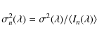
Figure 12:
Low-resolution spectra of T Cha. The panels on the left side display the whole range,
those on the right show the interval containing H |
| Open with DEXTER | |
7 Variability in the low-resolution spectra
Strong variability was also detected in our low-resolution spectroscopy.
We refer in particular to Table 4![]() , where we report the equivalent widths of
the H
, where we report the equivalent widths of
the H![]() and [O I]
and [O I]![]() 6300 Å lines, and to
Fig. 12, where a sample of low-resolution
spectra is shown
6300 Å lines, and to
Fig. 12, where a sample of low-resolution
spectra is shown![]() .
.
We note that during the May-June 1993 run, the star exhibited
spectacular changes between one night and the next. For instance, H![]() was observed to vary between weak absorption (
was observed to vary between weak absorption (
![]() )
on May 31,
to a very strong emission line (
)
on May 31,
to a very strong emission line (
![]() Å) on June 1.
The latter spectrum was also characterised by strong [O I] lines,
and the [N II] line was also present, while no emission lines were
detected in data acquired the two nights before.
Å) on June 1.
The latter spectrum was also characterised by strong [O I] lines,
and the [N II] line was also present, while no emission lines were
detected in data acquired the two nights before.
The spectacular variability of these lines is illustrated in
Fig. 13, where two low-resolution spectra, corresponding to
close to the maximum and minimum brightness of the star, just two nights apart,
are compared after normalising each of them to the flux at
![]() Å. We recall that these spectra are calibrated in
relative flux (see Sect. 3.2).
The variation in the continuum slope between the two dates is also remarkable,
in addition to the emission features appearing prominent when the
photospheric continuum looks fainter and heavily reddened.
Å. We recall that these spectra are calibrated in
relative flux (see Sect. 3.2).
The variation in the continuum slope between the two dates is also remarkable,
in addition to the emission features appearing prominent when the
photospheric continuum looks fainter and heavily reddened.
![\begin{figure}
\resizebox{9cm}{!}{\rotatebox{-90}{\includegraphics[width=9cm, trim = 10mm 10mm 10mm 10mm]{1073f13.ps}}}
\end{figure}](/articles/aa/full_html/2009/27/aa11073-08/img66.png) |
Figure 13:
Low-resolution spectra of T Cha near minimum (June 1, in red)
and maximum brightness (May 30, in blue).
The spectra are calibrated in relative flux and normalised to the flux at
|
| Open with DEXTER | |
![\begin{figure}
\par\includegraphics[width=9cm,trim = 0mm 15mm 0mm 0mm, clip]{1073f14a.eps}\par\includegraphics[width=9cm]{1073f14b.eps}
\end{figure}](/articles/aa/full_html/2009/27/aa11073-08/img67.png) |
Figure 14: Best-fit of spectral-type templates to the spectra shown in Fig. 13. The spectra of T Cha are shown as thin (black) lines, while the templates are shown as thick (red) lines. The corresponding values of total visual extinction, as derived from the two-parameter fit adopting a normal interstellar extinction law with RV=3.1, are also indicated for both the faint and bright stage, respectively. |
| Open with DEXTER | |
However, no change in the spectral type of the star is observed. To verify this, we used low-resolution spectra calibrated in relative flux, and applied the methods described in Alcalá et al. (2006) and Gandolfi et al. (2008) to determine simultaneously the spectral type and the visual extinction at the phases of minimum and maximum brightness, respectively. The result, shown in Fig. 14, is that the spectral type did not vary to within about half a sub-class, while the visual extinction changed from 1.2 mag in the bright phase to about 4.6 mag in the faint state, respectively. This corresponds to an extinction increase of at least 3.4 mag between the bright and faint states. By instead using the spectrum corresponding to the bright level as a template, an extinction of 3.3 mag is needed to reproduce the faint spectrum, and, apart from emission lines, the residual is indeed quite low (cf. Fig. 15).
We applied the same procedure to each of the low-resolution spectra and
determined the corresponding value of AV (see Table 4),
with estimated errors of about 10%.
This takes account of the uncertainty in the fit, as well as the relative
flux calibration, but not systematic effects caused by deviation of the
circumstellar extinction from the normal interstellar law, as shown in
Sect. 8.
The two panels of Fig. 16 show that a clear trend exists between the
amount of visual extinction and the intensity of the H![]() and
[O I] 6300 Å emission lines.
This indicates that the observed variations do not reflect intrinsic changes
in the stellar photosphere, but arise presumably from variable circumstellar
extinction, as can be inferred in Fig. 13 from the different
continuum slopes of two spectra taken near maximum (on 30 May 1993) and minimum
(on 1 Jun. 1993) brightness.
The histogram in Fig. 17 indicates that the highest extinction
events are relatively rare, while events with differential extinction below
1 mag are more frequent.
and
[O I] 6300 Å emission lines.
This indicates that the observed variations do not reflect intrinsic changes
in the stellar photosphere, but arise presumably from variable circumstellar
extinction, as can be inferred in Fig. 13 from the different
continuum slopes of two spectra taken near maximum (on 30 May 1993) and minimum
(on 1 Jun. 1993) brightness.
The histogram in Fig. 17 indicates that the highest extinction
events are relatively rare, while events with differential extinction below
1 mag are more frequent.
![\begin{figure}
\par\includegraphics[width=7.7cm,clip]{1073f15a.eps}
\includegr...
...cs[origin=rb,angle=-90,width=7.7cm,height=6.3cm,clip]{1073f15b.ps}
\end{figure}](/articles/aa/full_html/2009/27/aa11073-08/img68.png) |
Figure 15: The top panel shows the spectrum at the faint state as a thin (black) line, and the spectrum at the bright stage, used as a template, is shown as a thick (red) line. The lower panel shows the residual. The average residual and rms are indicated. The emission lines, not included in the deriving the average value of the residual, are marked. |
| Open with DEXTER | |
8 The spectral energy distribution
We constructed the observed SED of T Cha using all optical and
near-IR photometry available to us (Covino et al. 1996; Alcalá et al. 1993),
as well as data from public catalogues. In Fig. 18,
the SED is shown for wavelengths shorter than ![]() m.
We remark that photometric errors are smaller than the symbol size,
and the considerable scatter of the optical (
m.
We remark that photometric errors are smaller than the symbol size,
and the considerable scatter of the optical (
![]() bands)
data points reflects the significant variability of the star.
Although of smaller amplitude, variability in the near-IR (
bands)
data points reflects the significant variability of the star.
Although of smaller amplitude, variability in the near-IR (![]() bands)
can also be appreciated.
Therefore, relying on data that have not been acquired simultaneously
may be a limitation in the SED analysis.
bands)
can also be appreciated.
Therefore, relying on data that have not been acquired simultaneously
may be a limitation in the SED analysis.
At the brightest level, the observed J flux was lower than the expected stellar photospheric flux. However, we note that T Cha has not been monitored as extensively in the near-IR as in the optical. Therefore, the available data probably did not detect the brightest J flux. For that reason, the J flux was excluded from our SED-fitting. Excess emission is instead observed for wavelengths longer than the H band. The agreement of the Spitzer spectroscopy with the photometric data in the mid- and far-IR (cf. Fig. 19) indicates that there is no significant variability at longer wavelengths. This is expected in the case that the strong brightness and colour variations affecting the star are due to variable extinction of the stellar photosphere from inhomogeneous, circumstellar material.
By assuming variable extinction, we used relationships derived from
![]() photometry (Covino et al. 1996) to probe the dust column affecting the brightness
of T Cha.
In Table 4, we report the circumstellar extinction law for T Cha,
expressed by the total to selective extinction ratios,
photometry (Covino et al. 1996) to probe the dust column affecting the brightness
of T Cha.
In Table 4, we report the circumstellar extinction law for T Cha,
expressed by the total to selective extinction ratios,
![]() ,
derived from the differential brightness variations measured in the
,
derived from the differential brightness variations measured in the
![]() bands
(Covino et al. 1996).
The resulting value of RV deviates from the normal value (RV=3.1) for the diffuse
interstellar medium, which indicates different physical properties of the circumstellar
grains. In particular, a higher value of RV means a flatter extinction curve
(i.e., greyer extinction), and reveals the presence of larger grains, thus implying
probable grain growth and depletion of small grains (Draine 2008).
bands
(Covino et al. 1996).
The resulting value of RV deviates from the normal value (RV=3.1) for the diffuse
interstellar medium, which indicates different physical properties of the circumstellar
grains. In particular, a higher value of RV means a flatter extinction curve
(i.e., greyer extinction), and reveals the presence of larger grains, thus implying
probable grain growth and depletion of small grains (Draine 2008).
![\begin{figure}
\par\includegraphics[angle=-90,width=17cm,clip]{1073f16.ps}
\end{figure}](/articles/aa/full_html/2009/27/aa11073-08/img71.png) |
Figure 16:
Visual extinction derived from low-resolution flux-calibrated spectra versus the
equivalent width of H |
| Open with DEXTER | |
Therefore, in the following SED analysis, we considered more suitable the flux measurements corresponding to the brightest level of the star, shown in Fig. 19.
Disc models such as those by Robitaille et al. (2006,2007) do not take account of the presence of a partially evacuated inner hole or gap, so may be inadequate in reproducing the SED of transitional objects such as T Cha. Brown et al. (2007) found that the mid-IR spectrum of T Cha can be reproduced by a disc truncated at 0.08 AU with a gap between 0.2 and 15 AU, but they did not consider the strong variability of the object nor use the available millimetre data.
We explored the possibility of modelling the SED, simultaneously from
optical to millimetre wavelengths, using the CGPLUS prescription
by Dullemond et al. (2001). Starting from the stellar parameters in
Table 3, we constructed a grid of SEDs.
The results of the SED fitting are reported in Table 3
and the best-fit models are overplotted on the observed SED in
Fig. 19.
The dust opacities calculated by Laor & Draine (1993), modified to match the
Beckwith et al. (1990) opacity law at wavelengths longer than 100 ![]() m
were used. We note that a blackbody with
m
were used. We note that a blackbody with
![]() K better
reproduces the optical data.
Previous estimates of the disc mass based on single measurements at millimetre
wavelengths are in the range of
K better
reproduces the optical data.
Previous estimates of the disc mass based on single measurements at millimetre
wavelengths are in the range of
![]() -
-
![]() (Henning et al. 1993; Lommen et al. 2007), but our estimate reproduces well the observed data
for wavelengths longer than 60
(Henning et al. 1993; Lommen et al. 2007), but our estimate reproduces well the observed data
for wavelengths longer than 60 ![]() m. The disc radius is more poorly constrained,
but values between 100 and 150 AU provide quite reasonable results.
The latter is consistent with the 3.3 mm observations by Lommen et al. (2007)
that did not resolve the disc around T Cha.
We note that the disc radius adopted by Brown et al. (2007)
is a factor of two higher than the value derived here.
m. The disc radius is more poorly constrained,
but values between 100 and 150 AU provide quite reasonable results.
The latter is consistent with the 3.3 mm observations by Lommen et al. (2007)
that did not resolve the disc around T Cha.
We note that the disc radius adopted by Brown et al. (2007)
is a factor of two higher than the value derived here.
Although the model with a disc radius of 150 AU reproduces well
the observed SED at optical, far-IR, and millimeter wavelengths,
all the models predict too high flux between 10 and 30 ![]() m
relative to the observed SED.
Thus, despite our attempt to minimize the effects of colour changes by adopting
the brightest flux level in each band, we were unable to fit the complete SED
of T Cha with a simple reprocessing-disc model. This failure is probably caused
by excess emission in the near-IR. Therefore, the most plausible disc model
for reproducing the SED of T Cha is a disc with a gap, as proposed
by Brown et al. (2007).
m
relative to the observed SED.
Thus, despite our attempt to minimize the effects of colour changes by adopting
the brightest flux level in each band, we were unable to fit the complete SED
of T Cha with a simple reprocessing-disc model. This failure is probably caused
by excess emission in the near-IR. Therefore, the most plausible disc model
for reproducing the SED of T Cha is a disc with a gap, as proposed
by Brown et al. (2007).
Table 5:
Total to selective extinction ratios,
![]() ,
for T Cha,
derived from
,
for T Cha,
derived from
![]() photometry (Covino et al. 1996).
photometry (Covino et al. 1996).
![\begin{figure}
\par\includegraphics[angle=-90,width=8cm,clip]{1073f17.ps}
\end{figure}](/articles/aa/full_html/2009/27/aa11073-08/img80.png) |
Figure 17: Histogram of differential visual extinction. The most frequent value is around 0.5 mag, while the maximum observed is 3.3 mag. |
| Open with DEXTER | |
![\begin{figure}
\par\includegraphics[angle=-90,width=8cm,clip]{1073f18.ps}
\end{figure}](/articles/aa/full_html/2009/27/aa11073-08/img82.png) |
Figure 18:
Observed SED of T Cha for
|
| Open with DEXTER | |
![\begin{figure}
\par\includegraphics[angle=-90,width=8cm,clip]{1073f19.ps}
\end{figure}](/articles/aa/full_html/2009/27/aa11073-08/img83.png) |
Figure 19: Observed data-points used for SED fitting. Optical: symbols as in Fig. 18; IRAS: open triangles. Also superposed are IRS spectra (thin line). Three disc models, whose parameters are reported in Table 3, are represented by the solid, dashed and dotted lines, for different disc radii. |
| Open with DEXTER | |
9 Discussion and conclusions
Before discussing our interpretation of T Cha, we briefly summarise the most significant properties of the star derived from analysis of the spectroscopic observations presented here, complemented with published photometry and other data from public archives:
- a)
- we confirmed the spectral type G8 and a lithium abundance indicative of a very young age;
- b)
- we detected RV variations of almost 10 km s-1 on relatively short timescale,
but did not find any clear periodicity that could be related to orbital motion.
Besides that, the
 determinations obtained from FEROS observations
are consistent with the value of
determinations obtained from FEROS observations
are consistent with the value of  km s-1, except for a few
spectra in which the photospheric lines are significantly narrower,
yielding a
of
km s-1, except for a few
spectra in which the photospheric lines are significantly narrower,
yielding a
of  km s-1;
- c)
- strong variability in the main emission features (e.g., H,
H,
and
[O I] lines) on timescales comparable to that of photometric variability,
and a close correlation between the H
and [O I] line intensities are found;
- d)
- variations in the photospheric continuum slope are observed in connection with intensity changes in the main emission features (i.e., the line intensities strengthen when the star reddens and fades);
- e)
- clearly evident relationships between brightness and colours based on optical photometry (Covino et al. 1996; Alcalá et al. 1993) have allowed us to derive a circumstellar extinction law characterised by RV=5.5 and infer the presence of large circumstellar dust grains;
- f)
- the observed SED, showing a dip at mid-IR wavelengths, is typical of a transitional disc. SED modelling has confirmed the presence of a disc with a gap and a high inclination angle, as first indicated by Brown et al. (2007).
Table 6: In the upper table, we report the estimated stellar properties, and in the lower table, the stellar and disc parameters resulting from SED-fitting using Dullemond et al. (2001) model.
![\begin{figure}
\par\includegraphics[width=14cm,clip]{1073f20.ps}
\end{figure}](/articles/aa/full_html/2009/27/aa11073-08/img102.png) |
Figure 20: Comparison between T Cha spectra observed in two different epochs: in blue the spectrum observed on 14 Feb. 2002, in red the one observed on 26 Apr. 2004, in black the difference between the two. Various spectral lines at different wavelengths are marked. |
| Open with DEXTER | |
But what is the source for the bulk H![]() emission in T Cha?
It is generally accepted that the strong H
emission in T Cha?
It is generally accepted that the strong H![]() emission line in
T Tauri stars is due to mass accretion, which leads to UV excess
emission and photospheric continuum veiling (Hartigan et al. 1995).
Transitional objects, however, have more evolved discs in which accretion
should decrease significantly with respect to the earlier CTTS phase.
In T Cha, no veiling is apparently detected, not even in the stages of
strong H
emission line in
T Tauri stars is due to mass accretion, which leads to UV excess
emission and photospheric continuum veiling (Hartigan et al. 1995).
Transitional objects, however, have more evolved discs in which accretion
should decrease significantly with respect to the earlier CTTS phase.
In T Cha, no veiling is apparently detected, not even in the stages of
strong H![]() emission (see Figs. 5, 15,
and 20) suggesting very low or no mass accretion.
However, the non-detection of veiling in T Cha may also caused by
the relatively high continuum flux emitted by its G8 photosphere.
Hence, we cannot exclude the possibility that erratic accretion episodes
are caused by instabilities in the inner disc, in which infalling gas
produces the variable redshifted absorption features that we observe
in the H
emission (see Figs. 5, 15,
and 20) suggesting very low or no mass accretion.
However, the non-detection of veiling in T Cha may also caused by
the relatively high continuum flux emitted by its G8 photosphere.
Hence, we cannot exclude the possibility that erratic accretion episodes
are caused by instabilities in the inner disc, in which infalling gas
produces the variable redshifted absorption features that we observe
in the H![]() line profile.
However, the [O I]
line profile.
However, the [O I] ![]() 6300 Å emission, which corresponds
to a luminosity of
6300 Å emission, which corresponds
to a luminosity of
![]() ,
implies
the presence of strong winds, although the width of the line
(
,
implies
the presence of strong winds, although the width of the line
(![]() 100 km s-1, see Fig. 6) is at the lower limit
of a typical high-velocity component (Hartigan et al. 1995).
It is probable that the bulk of the H
100 km s-1, see Fig. 6) is at the lower limit
of a typical high-velocity component (Hartigan et al. 1995).
It is probable that the bulk of the H![]() emission observed in T Cha
is also produced in a wind, as reported for some Herbig Ae stars (Kraus et al. 2008).
Moreover, the H
emission observed in T Cha
is also produced in a wind, as reported for some Herbig Ae stars (Kraus et al. 2008).
Moreover, the H![]() versus [O I] correlation shown in
Fig. 7 is more easily explained in terms of variable
circumstellar extinction, rather than variable accretion.
versus [O I] correlation shown in
Fig. 7 is more easily explained in terms of variable
circumstellar extinction, rather than variable accretion.
By both assuming variable circumstellar extinction, and adopting the relation
![]() and the extinction cross-section per H nucleon
for RV=5.5,
and the extinction cross-section per H nucleon
for RV=5.5,
![]() cm2/H, given by
Draine (2003), we estimate the column density for an obscuring clump
to be
cm2/H, given by
Draine (2003), we estimate the column density for an obscuring clump
to be
![]() cm-2.
By also assuming the maximum observed differential extinction of 3.3 mag,
we obtain a hydrogen column density
cm-2.
By also assuming the maximum observed differential extinction of 3.3 mag,
we obtain a hydrogen column density
![]() cm-2.
We can estimate the mass of the obscuring clumps,
cm-2.
We can estimate the mass of the obscuring clumps,
![]() ,
by assuming
that they cover completely the photospheric disc of the star.
Using the stellar radius reported in Table 3, the result is
,
by assuming
that they cover completely the photospheric disc of the star.
Using the stellar radius reported in Table 3, the result is
![]() g, i.e., of the order of
g, i.e., of the order of
![]()
![]() .
Similarly, assuming the most frequent differential circumstellar extinction
from the histogram in Fig. 17, the result would be
.
Similarly, assuming the most frequent differential circumstellar extinction
from the histogram in Fig. 17, the result would be
![]()
![]() .
In contrast, the mass
of asteroid 253 Mathilde is
.
In contrast, the mass
of asteroid 253 Mathilde is
![]()
![]() (Yeomans et al. 1998).
(Yeomans et al. 1998).
Finally, could the RV variations in T Cha becaused by a low-mass companion?
Some PMS stars with transitional discs, such as CoKu Tau/4, have been
discovered to be binaries (e.g., Ireland & Kraus 2008). The inner
edge of circumbinary discs is believed to be set by dynamical truncation.
In the case of CoKu Tau/4, where the binary separation is about 8 AU,
the truncation radius would be of the order of 13-16 AU, depending on
the eccentricity of the binary (Ireland & Kraus 2008).
As concluded from our analysis of the CCF bisector, the RV variation of T Cha
is about 10 km s-1. A very low-mass object, say a 0.05 ![]() brown dwarf on a circular orbit with a radius of about 0.1 AU may cause
this variation, producing a disc truncation radius of about 0.2 AU,
consistent with the inner disc edge proposed by Brown et al. (2007).
However, no obvious periodicity is detected in our RV measurements.
On the other hand, the gap proposed by Brown et al. (2007) cannot be explained
in terms of truncation by a companion at a separation of about 10-15 AU.
At such separation, a 0.9
brown dwarf on a circular orbit with a radius of about 0.1 AU may cause
this variation, producing a disc truncation radius of about 0.2 AU,
consistent with the inner disc edge proposed by Brown et al. (2007).
However, no obvious periodicity is detected in our RV measurements.
On the other hand, the gap proposed by Brown et al. (2007) cannot be explained
in terms of truncation by a companion at a separation of about 10-15 AU.
At such separation, a 0.9 ![]() star would be necessary to produce
the observed RV variation. An object of that mass and separation
would have been eventually detected either by us as a spectroscopic binary,
or by Köhler (2001) in his speckle survey. Thus, the
gap of the transitional disc in T Cha is probably not the result of dynamical
truncation due to a binary companion.
In any case, the presence of a lower-mass (stellar or substellar) companion
cannot be definitely excluded because a quasi-periodicity of about 3 days
is clearly evident throughout the entire data-set of T Cha.
On the other hand, T Cha is a relatively fast rotator (
star would be necessary to produce
the observed RV variation. An object of that mass and separation
would have been eventually detected either by us as a spectroscopic binary,
or by Köhler (2001) in his speckle survey. Thus, the
gap of the transitional disc in T Cha is probably not the result of dynamical
truncation due to a binary companion.
In any case, the presence of a lower-mass (stellar or substellar) companion
cannot be definitely excluded because a quasi-periodicity of about 3 days
is clearly evident throughout the entire data-set of T Cha.
On the other hand, T Cha is a relatively fast rotator (
![]() km s-1)
and a magnetically active (
km s-1)
and a magnetically active (
![]() 30 erg s-1) PMS star.
Therefore, the observed RV variations might be alternatively induced by stellar spots,
as in the case of the WTTs V410 Tau (Stelzer et al. 2003).
Otherwise, we cannot exclude the possibility that the same circumstellar
inhomogeneities responsible for the variable extinction may also alter the symmetry
of the photospheric lines, and cause apparent RV shifts due to a sort of Rossiter
effect, as in eclipsing binaries, which occurs when the stellar photosphere is
partially obscured.
In all cases, the presence of an inner disc characterised by a clumpy structure
and the evidence of grain growth both indicate that T Cha is a likely candidate
to host planet formation.
30 erg s-1) PMS star.
Therefore, the observed RV variations might be alternatively induced by stellar spots,
as in the case of the WTTs V410 Tau (Stelzer et al. 2003).
Otherwise, we cannot exclude the possibility that the same circumstellar
inhomogeneities responsible for the variable extinction may also alter the symmetry
of the photospheric lines, and cause apparent RV shifts due to a sort of Rossiter
effect, as in eclipsing binaries, which occurs when the stellar photosphere is
partially obscured.
In all cases, the presence of an inner disc characterised by a clumpy structure
and the evidence of grain growth both indicate that T Cha is a likely candidate
to host planet formation.
Acknowledgements
We thank the user support group of ESO/La Silla. We are grateful to Rainer Wichmann for providing us with the series of FEROS spectra of March 1999. This research has made use of SIMBAD and VIZIER databases, operated at CDS, Strasbourg, France. This publication makes use of data products from the Two Micron All Sky Survey, which is a joint project of the University of Massachusetts and the Infrared Processing and Analysis Center/California Institute of Technology, funded by the National Aeronautics and Space Administration and the National Science Foundation. This work is based in part on archivial data obtained with the Spitzer Space Telescope, which is operated by the Jet Propulsion Laboratory, California Institute of Technology under a contract with Nasa. Financial support from INAF (PRIN 2007: From active accretion to debris discs) is acknowledged. We thank the anonymous referee for constructive criticism and comments that helped to improve this paper.
References
- Alcalá, J. M., Covino, E., Franchini, M., et al. 1993, A&A, 272, 225 [NASA ADS]
- Alcalá, J. M., Krautter, J., Schmitt, J. H. M. M., et al. 1995, A&AS, 114, 109 [NASA ADS]
- Alcalá, J. M., Spezzi, L., Frasca, A., et al. 2006, A&A, 453, 1 [NASA ADS] [CrossRef] [EDP Sciences] (In the text)
- Alencar, S. H. P., & Batalha, C. 2002, ApJ, 571, 378 [NASA ADS] [CrossRef]
- Alexander, R. D., & Armitage, P. J., 2007, MNRAS, 375, 500 [NASA ADS] [CrossRef]
- Appenzeller, I., & Mundt, R. 1989, A&ARv, 1, 291 [NASA ADS]
- Beckwith, S. V. W., Sargent, A. I., Chini, R. S., & Guesten, R. 1990, AJ, 99, 924 [NASA ADS] [CrossRef] (In the text)
- Bertout, C. 2000, A&A, 363,984 (In the text)
- Bertout, C., Siess, L., & Cabrit, S., 2007, A&A, 473L, 21 [NASA ADS] [CrossRef] (In the text)
- Bessel, M. 1979, PASP, 91, 589 [NASA ADS] [CrossRef] (In the text)
- Bouret, J.-C., & Catala, C. 2000, A&A, 259, 1011 [NASA ADS]
- Bouvier, J., Grankin, K. N., Alencar, S. H. P., et al. 2003, A&A, 409, 169 [NASA ADS] [CrossRef] [EDP Sciences] (In the text)
- Brown, J. M., Blake, G. A., Dullemond, C. P., et al. 2007, ApJ, 664, 107 [NASA ADS] [CrossRef]
- Calvet, N., & Hartmann, L. 1992, ApJ, 386, 239 [NASA ADS] [CrossRef]
- Calvet, N., Hartmann, L., & Hewett, R. 1992, ApJ, 386, 229 [NASA ADS] [CrossRef]
- Cardelli, J. A., Clayton, G. C., & Mathis, J. S. 1989, AJ, 345, 245 [NASA ADS] [CrossRef]
- Chiang, E. I., & Goldreich, P. 1997, ApJ, 490, 368 [NASA ADS] [CrossRef]
- Cieza, L., Padgett, D., Stapelfeldt, K. R., et al. 2007, ApJ, 667, 308 [NASA ADS] [CrossRef]
- Clarke, C. J., Gendrin, A., & Sotomayor, M. 2001, MNRAS, 328, 485 [NASA ADS] [CrossRef]
- Covino, E., Terranegra, L., Franchini, M., Chavarria-K., C., & Stalio, R. 1992, A&AS, 94, 273 [NASA ADS]
- Covino, E., Alcala, J. M., Krautter, J., Terranegra, L., & Wichmann, R. 1994, Proceedings of a Conference honoring Hans Elsässer, Disks and Outflows Around Young Stars, ed. S. V. W. Beckwith, J. Staude, A. Quetz, & A. Natta, Lecture Notes in Physics, 465, 343
- Covino, E., Alcala, J. M., Allain, S., et al. 1997, A&A, 328, 187 [NASA ADS] (In the text)
- Cieza, L. A. 2008, ASPC, 393, 35 [NASA ADS]
- D'Alessio, P., Calvet, N., Hartmann, L., Lizano, S., & Cantó, J. 1999, ApJ, 527, 893 [NASA ADS] [CrossRef]
- Dall, T. H., Santos, N. C., Arentoft, T., et al. 2006, A&A, 454, 341 [NASA ADS] [CrossRef] [EDP Sciences]
- Draine, B. T. 2003, ARA&A, 41, 241 [NASA ADS] [CrossRef] (In the text)
- Draine, B. T. 2008, Space Sci. Rev., in press (In the text)
- Dullemond, C. P., Dominik, C., & Natta, A. 2001, ApJ, 560, 957 [NASA ADS] [CrossRef] (In the text)
- Dullemond, C. P., van den Ancker, M. E., Acke, B., & van Boekel, R. 2003, ApJ, 588, 360 [CrossRef]
- Dullemond, C. P., & Dominik, C. 2005, A&A, 434, 971 [NASA ADS] [CrossRef] [EDP Sciences]
- Edwards, S., Hartigan, P., Ghandour, L., & Andrulis, C. 1994, AJ, 108, 1056 [NASA ADS] [CrossRef]
- Espaillat, C., Calvet, N., Luhman, K. L., Muzerolle, J., & D'Alessio, P. 2008, ApJ, 682, 125 [NASA ADS] [CrossRef]
- Esposito, M., Covino, E., Alcalá, J. M., Guenther, E. W., & Schisano, E. 2007, MNRAS, 376, 1805 [NASA ADS] [CrossRef]
- Evans, N. J. II, Dunham, M. M., Jørgensen, J. K., et al. 2008, ApJ, in press [arXiv:0811.1059]
- Franchini, M., Covino, E., Stalio, R., Terranegra, L., & Chavarria-K., C. 1992, A&A, 256, 525 [NASA ADS]
- Frink, S., Roeser, S., Alcalá, J. M., Covino, E., & Brandner, W. 1998, A&A, 338, 442 [NASA ADS] (In the text)
- Furlan, E., Hartmann, L., Calvet, N., D'Alessio, P., et al. 2006, ApJS, 165, 568 [NASA ADS] [CrossRef]
- Gahm, G. F., Fischerstrom, C., Lindroos, K. P., & Liseau, R. 1989, A&A, 211, 115 [NASA ADS] (In the text)
- Gandolfi, D., Alcalá, L. S., et al. 2008, ApJ, 687, 1303 [NASA ADS] [CrossRef] (In the text)
- Geers, V. C., Augereau, J. C., Pontoppidan, K. M., et al. 2006, A&A, 459, 545 [NASA ADS] [CrossRef] [EDP Sciences]
- Gras-Velazquez, A., & Ray, T. P. 2005, A&A, 443, 541 [NASA ADS] [CrossRef] [EDP Sciences]
- Greene, T. P., Wilking, B. A., André, P., et al. 1994, ApJ, 434, 614 [NASA ADS] [CrossRef]
- Gray, D. F. 2005, The Observation and Analysis of Stellar Photospheres (3rd ed.: Cambridge: Cambridge Univ.)
- Gregorio-Hetem, J., Lepine, J. R. D., Quast, G. R., Torres, C. A. O., & de La Reza, R. 1992, AJ, 103, 549 [NASA ADS] [CrossRef] (In the text)
- Grinin, V. P. 1988, PAZh, 14 ,65 (In the text)
- Guenther, E. W., Esposito, M., Mundt, R., et al. 2007, A&A, 467, 1147 [NASA ADS] [CrossRef] [EDP Sciences]
- Hartmann, L., Avrett, E. H., Loeser, R., & Calvet, N. 1990, ApJ, 349, 168 [NASA ADS] [CrossRef]
- Hartigan, P., Hartmann, L., Kenyon, S., & Hewett, R. 1989, ApJS, 70, 899 [NASA ADS] [CrossRef]
- Hartigan, P., Edwards, S., & Ghandour, L. 1995, ApJ, 452, 736 [NASA ADS] [CrossRef] (In the text)
- Henning, T., Pfau, W., Zinnecker, H., & Prusti, T. 1993, A&A, 346, 205
- Herbst, W., Herbst, D. K., Grossman, E. J., & Weinstein, D. 1994, AJ, 108, 1906 [NASA ADS] [CrossRef] (In the text)
- Herbst, W., & Shevchenko, V. S. 1999, AJ, 118, 1043 [NASA ADS] [CrossRef] (In the text)
- Hermann, F., & Krikov, A. V. 2007, A&A, 829, 839 (In the text)
- Hirth, G. A., Mundt, R., Solf, J., & Ray, Th. P. 1994, ApJ, 427, 99 [NASA ADS] [CrossRef]
- Hoffmeister, C. 1958, Veroff. Sonnborg, 3, 342 [NASA ADS]
- Hollenbach, D. J., Yorke, H. W., & Johnstone, D. 2000 in Protostars and Planets IV (Book - Tucson: University of Arizona Press), ed. V. Mannings, A. P. Boss, & S. S. Russell, 401
- Ireland., M. J., & Kraus, A. L. 2008, ApJ, 678, 59 [NASA ADS] [CrossRef] (In the text)
- Isella, A., Testi, L., & Natta, A. 2006, A&A, 451, 951 [NASA ADS] [CrossRef] [EDP Sciences]
- Johns, C. M., & Basri, G. 1995, AJ, 109, 2800 [NASA ADS] [CrossRef] (In the text)
- Kessler-Silacci, J., Augereau, J.-C., Dullemond, C.P., et al. 2006, ApJ, 639, 275 [NASA ADS] [CrossRef]
- Kraus, S., Hofmann, K.-H., Benisty, M., et al. 2008, A&A, 489, 1157 [NASA ADS] [CrossRef] [EDP Sciences] (In the text)
- Kenyon, S. J., & Hartmann, L. 1995, ApJS, 101, 117 [NASA ADS] [CrossRef] (In the text)
- Köhler, R. 2001, AJ, 122, 3325 [NASA ADS] [CrossRef] (In the text)
- Lada, C. J., Muench, A. A., Luhman, K. L., et al. 2006, AJ, 131, 1574 [NASA ADS] [CrossRef]
- Laor, A., & Draine, B. T. 1993, ApJ, 402, 441 [NASA ADS] [CrossRef] (In the text)
- Lommen, D., Wright, C. M., Maddison, S. T., et al. 2007, A&A, 462, 211 [NASA ADS] [CrossRef] [EDP Sciences]
- Mauder, H., & Sosna, F. M. 1975, IBVS, 1049
- Merín, B., et al. 2008, in prep.
- Millan-Gabet, R., et al. 2007, in Protostars & Planets V, ed. B. Reipurth, et al. (Tucson: Univ. Arizona Press), 539 (In the text)
- Mitskevich, A. S., Natta, A., & Grinin, V. P. 1993, ApJ, 404, 751 [NASA ADS] [CrossRef]
- Morel, M., & Magnenat, P. 1978, Astron. Astrophys. Suppl., 34, 477 [NASA ADS] (In the text)
- Muzzerolle, J., Calvet, N., & Hartmann, L. 2001, ApJ, 550, 944 [NASA ADS] [CrossRef]
- Najita, J. R., Stephen, E. S., & Muzerolle, J. 2007, MNRAS, 378, 369 [NASA ADS] [CrossRef]
- Natta, A., Grinin, V., & Mannings, V. 2000, in Protostars and Planets IV (Book - Tucson: University of Arizona Press), 559
- Natta, A., Prusti, T., Neri, R., et al. 2001, A&A, 371, 186 [NASA ADS] [CrossRef] [EDP Sciences]
- Natta, A., Testi, L., Muzerolle, J., et al. 2004, A&A, 424, 603 [NASA ADS] [CrossRef] [EDP Sciences] (In the text)
- Nordström, B., Mayor, M., Andersen, J., et al. 2004, A&A, 418, 989 [NASA ADS] [CrossRef] [EDP Sciences] (In the text)
- Palla, F., & Stahler, S. W. 1999, ApJ, 525, 772 [NASA ADS] [CrossRef]
- Pavlenko, Y. V., & Magazzú, A. 1996, A&A, 311, 961 [NASA ADS] (In the text)
- Pickles, A. J. 1998, PASP, 110, 863 [NASA ADS] [CrossRef]
- Queloz, D., Henry, G. W., Sivan, J. P., et al. 2001, A&A, 379, 279 [NASA ADS] [CrossRef] [EDP Sciences] (In the text)
- Reipurth, B., Pedrosa, A., & Lago, M. T. V. T. 1996, A&AS, 120, 229 [NASA ADS] [CrossRef] [EDP Sciences]
- Robitaille, T. P., Whitney, B. A., Indebetouw, R., Wood, K., & Denzmore, P. 2006, ApJS, 167, 256 [NASA ADS] [CrossRef]
- Robitaille, T. P., Whitney, B. A., Indebetouw, R., & Wood, K. 2007, ApJS, 169, 328 [NASA ADS] [CrossRef]
- Rodgers, B., Wooden, D. H., Grinin, V., Shakhovsky, D., & Natta, A. 2002, ApJ, 564, 405 [NASA ADS] [CrossRef] (In the text)
- Santos, N. C., Mayor, M., Naef, D., et al. 2002, A&A, 392, 215 [NASA ADS] [CrossRef] [EDP Sciences]
- Scargle, J. D. 1982, ApJ, 263, 835 [NASA ADS] [CrossRef] (In the text)
- Shu, F., Najita, J., Ostriker, E., et al. 1994, ApJ, 429, 781 [NASA ADS] [CrossRef]
- Sicilia-Aguilar, A., Hartmann, L. W., Watson, D., et al. 2007, ApJ, 659, 1637 [NASA ADS] [CrossRef]
- Stelzer, B., Fernández, M., Costa, V. M., et al. 2003, A&A, 411, 517 [NASA ADS] [CrossRef] [EDP Sciences] (In the text)
- Terranegra, L., Morale, F., Spagna, A., Massone, G., & Lattanzi, M. G. 1999, A&A, 341, L79 [NASA ADS] (In the text)
- Toner, C. G., & Gray, D. F. 1988, ApJ, 334, 1008 [NASA ADS] [CrossRef]
- Vinkovic, D., & Jurkic, T. 2007, ApJ, 658, 462 [NASA ADS] [CrossRef] (In the text)
- White, R. J., & Basri, G. 2003, ApJ, 582, 1109 [NASA ADS] [CrossRef] (In the text)
- Yeomans, D. K., Antreasian, P. G., Barriot, J.-P., et al. 1998, Science, 289, 2085 [NASA ADS] [CrossRef] (In the text)
Online Material
Table 1: Journal of FEROS observations and radial velocity measurements.
Table 2:
Radial velocity determinations, both from gaussian fit and bisector method, and equivalent widths of H![]() and [O I] 6300 Å measured on FEROS spectra.
and [O I] 6300 Å measured on FEROS spectra.
Table 4:
Equivalent widths of H![]() and [O I] 6300 Å
measured on the low-resolution spectra (see the atlas in electronic form)
and corresponding total extinction, AV, obtained as described in
Sect. 8.
and [O I] 6300 Å
measured on the low-resolution spectra (see the atlas in electronic form)
and corresponding total extinction, AV, obtained as described in
Sect. 8.
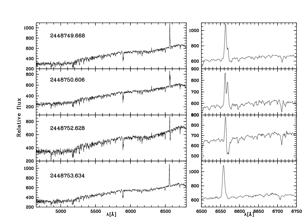 |
Figure 21:
Atlas of low-resolution spectra of T Cha. The panels on the left side display the whole range,
those on the right show the interval containing H |
| Open with DEXTER | |
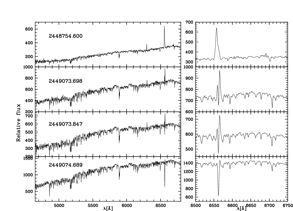 |
Figure 22: Atlas of low-resolution spectra of T Cha, continue. |
| Open with DEXTER | |
 |
Figure 23: Atlas of low-resolution spectra of T Cha, continue. |
| Open with DEXTER | |
 |
Figure 24: Atlas of low-resolution spectra of T Cha, continue. |
| Open with DEXTER | |
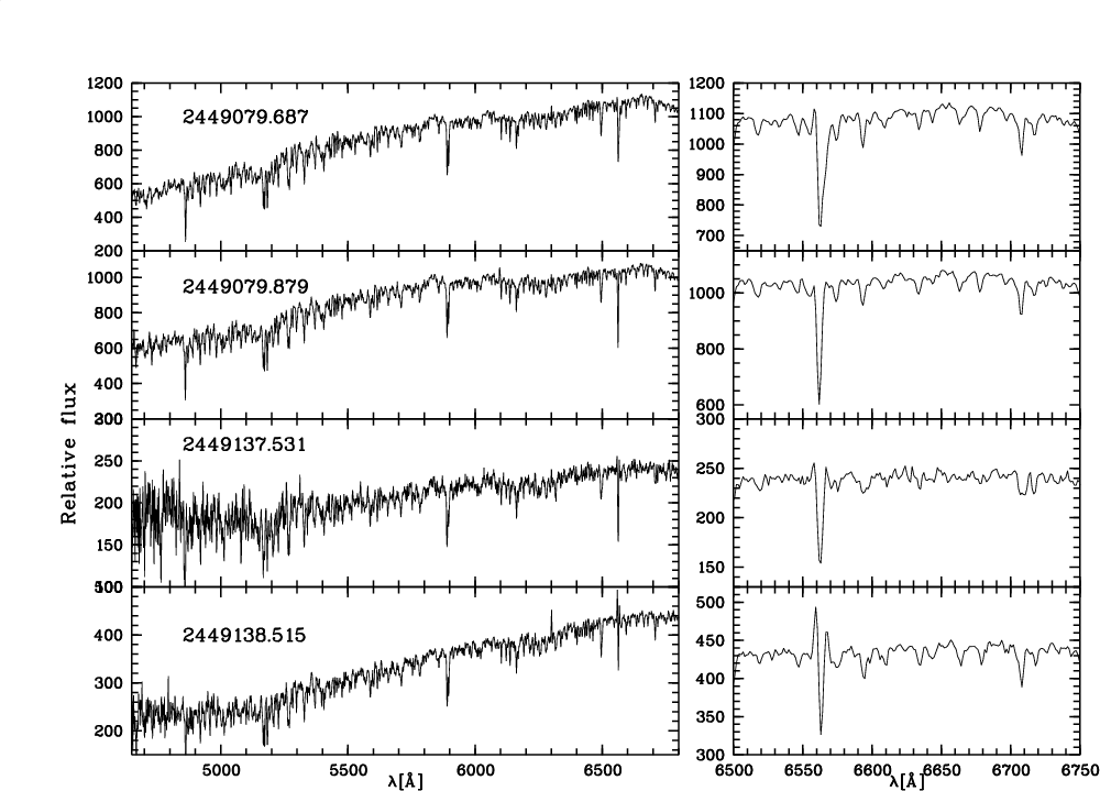 |
Figure 25: Atlas of low-resolution spectra of T Cha, continue. |
| Open with DEXTER | |
 |
Figure 26: Atlas of low-resolution spectra of T Cha, continue. |
| Open with DEXTER | |
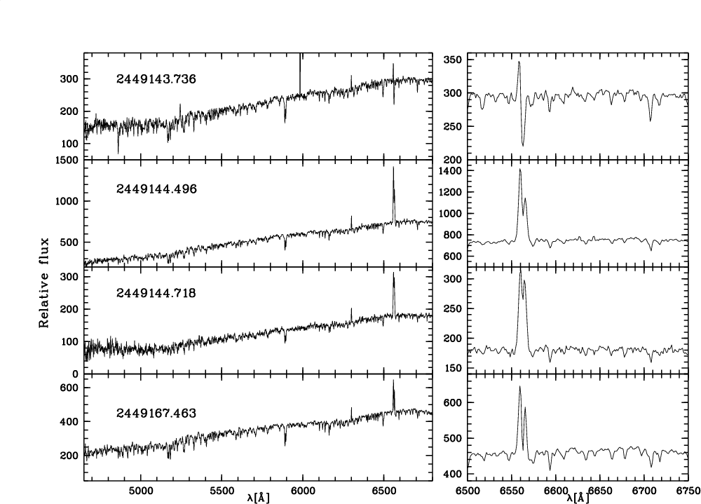 |
Figure 27: Atlas of low-resolution spectra of T Cha, continue. |
| Open with DEXTER | |
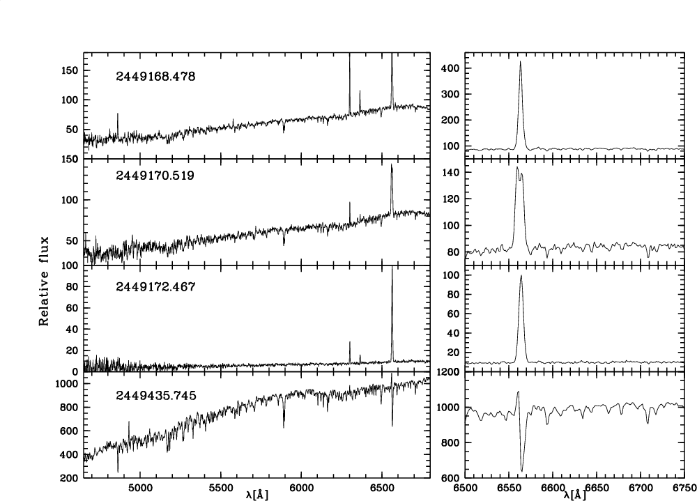 |
Figure 28: Atlas of low-resolution spectra of T Cha, continue. |
| Open with DEXTER | |
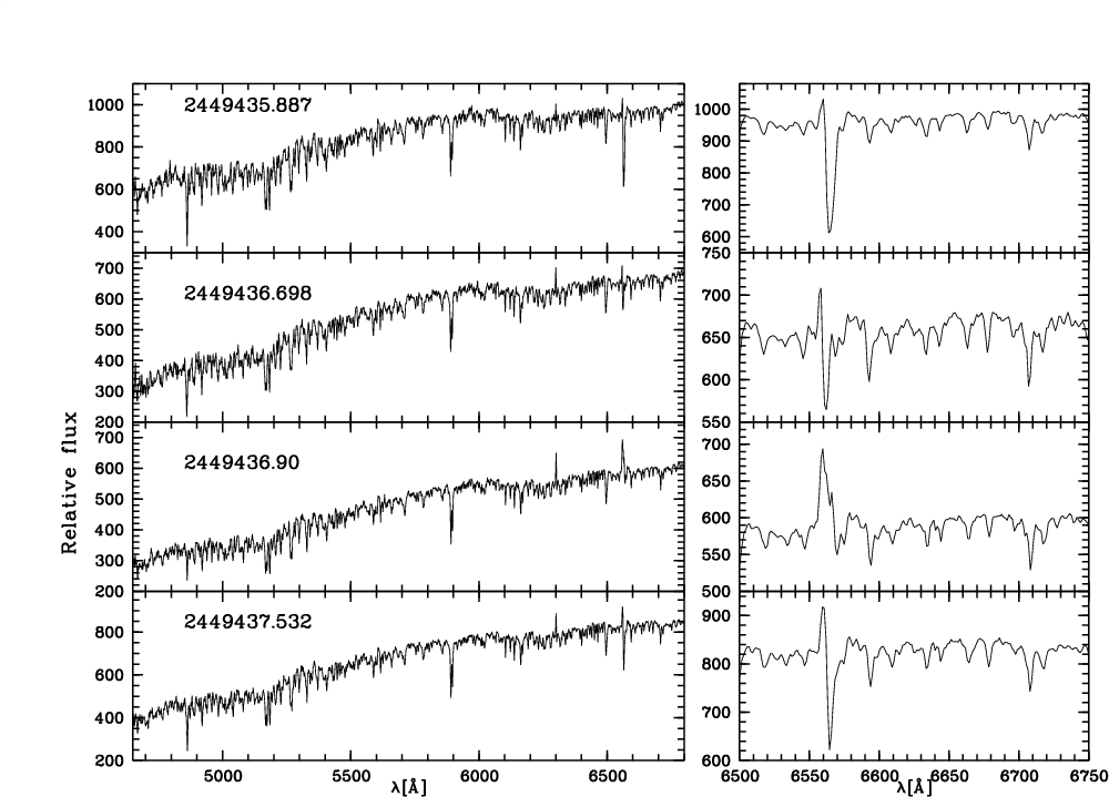 |
Figure 29: Atlas of low-resolution spectra of T Cha, continue. |
| Open with DEXTER | |
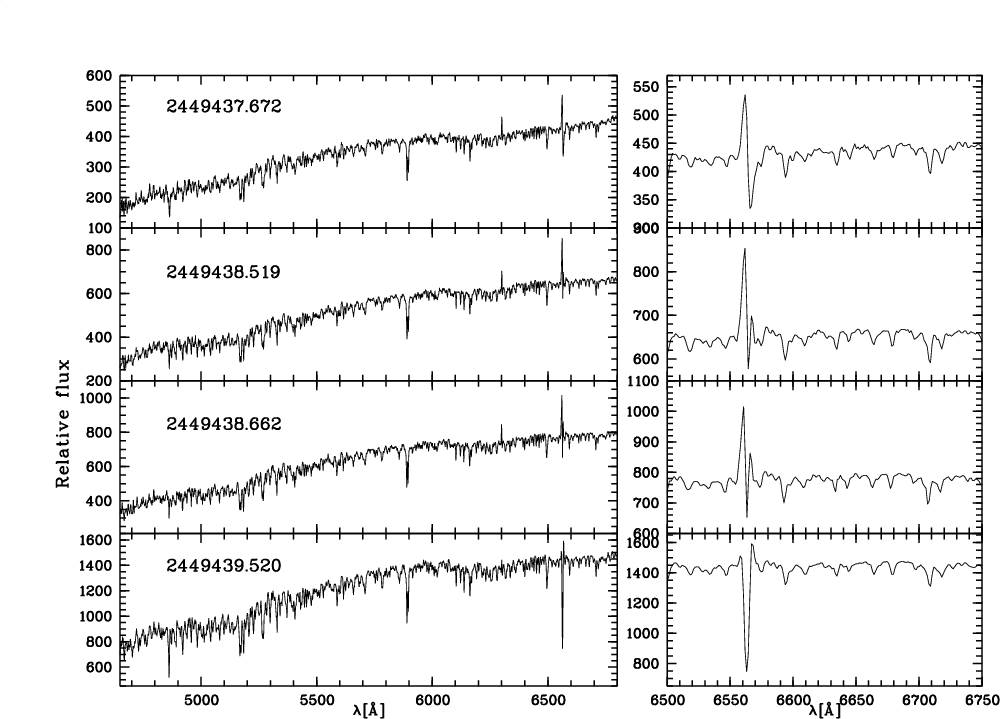 |
Figure 30: Atlas of low-resolution spectra of T Cha, continue. |
| Open with DEXTER | |
![\begin{figure}
\par\includegraphics[origin=rb,angle=-90,width=17cm,height=10cm,clip]{1073f31.ps}
\end{figure}](/articles/aa/full_html/2009/27/aa11073-08/img136.png) |
Figure 31: Atlas of low-resolution spectra of T Cha, continue. |
| Open with DEXTER | |
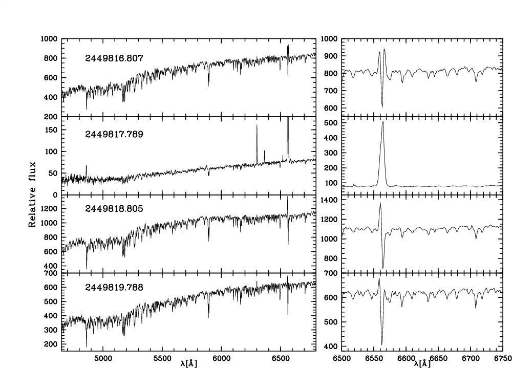 |
Figure 32: Atlas of low-resolution spectra of T Cha, continue. |
| Open with DEXTER | |
Footnotes
- ...
T Chamaeleontis
- Based on observations obtained at the European Southern Observatory at La Silla, Chile in program 63.I-0045(A); 65.I-0089(A); 66.C-0616(A); 67.C-0155(A); 67.C-0155(B); 68.C-0292(A); 69.C-0207(A); 70.C-0163(A); 073.C-0355(A); 074.A-9018(A); 075.C-0399(A-F).
- ...
- Tables 1, 2 and 4, and Figs. 21-32 are only available in electronic form via http://www.aanda.org
- ... ESO-MIDAS
- Munich Image Data Analysis System.
- ...
site
- http://www.ls.eso.org/lasilla/sciops/2p2/E2p2M/FEROS
- ... span
- All RV measurements are reported in Table 2, available electronically.
- ... spectra
- Reported in Table 2, only available in electronic form.
- ... 2002)
- Conventionally, a negative EW indicates line in emission.
- ...
- Available only in electronic form.
- ... shown
- The full atlas of low-resolution spectra is reported in Fig. 21, only in electronic form.
All Tables
Table 3: Equivalent widths of [O I] 6300 Å measured in CASPEC spectra (Covino et al. 1996) and line luminosity derived using simultaneous R-band photometry.
Table 5:
Total to selective extinction ratios,
![]() ,
for T Cha,
derived from
,
for T Cha,
derived from
![]() photometry (Covino et al. 1996).
photometry (Covino et al. 1996).
Table 6: In the upper table, we report the estimated stellar properties, and in the lower table, the stellar and disc parameters resulting from SED-fitting using Dullemond et al. (2001) model.
Table 1: Journal of FEROS observations and radial velocity measurements.
Table 2:
Radial velocity determinations, both from gaussian fit and bisector method, and equivalent widths of H![]() and [O I] 6300 Å measured on FEROS spectra.
and [O I] 6300 Å measured on FEROS spectra.
Table 4:
Equivalent widths of H![]() and [O I] 6300 Å
measured on the low-resolution spectra (see the atlas in electronic form)
and corresponding total extinction, AV, obtained as described in
Sect. 8.
and [O I] 6300 Å
measured on the low-resolution spectra (see the atlas in electronic form)
and corresponding total extinction, AV, obtained as described in
Sect. 8.
All Figures
| |
Figure 1:
Changes in the CCF in the period 19-23 May 2000, in two different
wavelength ranges. The different colours refer to the following dates:
19 May (
|
| Open with DEXTER | |
| In the text | |
| |
Figure 2:
CCF peaks between 16 and 22 May 1999 ( upper panel).
Velocity is relative to the template star.
The different colours refer to the following dates: 16 May (
|
| Open with DEXTER | |
| In the text | |
| |
Figure 3: The radial velocity measurements from Gaussian-fit method versus the ``bisector velocity span'' (i.e. the difference between the upper and bottom bisector mean velocities) are plotted in the left panel. The right panel shows, instead, the mean radial velocity of the CCF bisector bottom versus the ``bisector velocity span''. |
| Open with DEXTER | |
| In the text | |
| |
Figure 4: Projected rotational velocity from CCF Gaussian-fit calibration versus FWHM of the CCF peak. Only the data of the highest S/N are considered here. |
| Open with DEXTER | |
| In the text | |
| |
Figure 5:
Spectrum of T Cha obtained on 14 Feb. 2002.
The green line represents the spectrum of the template (HD 152 391 G8.5V)
artificially broadened for rotation.
In each panel is also shown the residual spectrum after subtraction.
Slight residuals in strong spectral features are mainly due to uncertainties
in the normalization to the continuum. The spectrum, with a good S/N,
shows a redshifted absorption component at H |
| Open with DEXTER | |
| In the text | |
| |
Figure 6: Examples of residual line profiles of T Cha in velocity scale. The vertical dotted line marks the rest position in the star frame. |
| Open with DEXTER | |
| In the text | |
| |
Figure 7: Correlations between intensities of the most prominent emission lines measured in the FEROS spectra. |
| Open with DEXTER | |
| In the text | |
| |
Figure 8:
Line profiles ( left panels) and corresponding variance and normalized variance profiles
( right panels) for H |
| Open with DEXTER | |
| In the text | |
| |
Figure 9:
Equivalent widths of the main emission lines during the runs displayed
in Fig. 8. The left scale refers to H |
| Open with DEXTER | |
| In the text | |
| |
Figure 10:
Variations in position of the central peak emission and the two absorptions of H |
| Open with DEXTER | |
| In the text | |
| |
Figure 11:
Two-dimensional maps of the correlation matrices of H |
| Open with DEXTER | |
| In the text | |
| |
Figure 12:
Low-resolution spectra of T Cha. The panels on the left side display the whole range,
those on the right show the interval containing H |
| Open with DEXTER | |
| In the text | |
| |
Figure 13:
Low-resolution spectra of T Cha near minimum (June 1, in red)
and maximum brightness (May 30, in blue).
The spectra are calibrated in relative flux and normalised to the flux at
|
| Open with DEXTER | |
| In the text | |
| |
Figure 14: Best-fit of spectral-type templates to the spectra shown in Fig. 13. The spectra of T Cha are shown as thin (black) lines, while the templates are shown as thick (red) lines. The corresponding values of total visual extinction, as derived from the two-parameter fit adopting a normal interstellar extinction law with RV=3.1, are also indicated for both the faint and bright stage, respectively. |
| Open with DEXTER | |
| In the text | |
| |
Figure 15: The top panel shows the spectrum at the faint state as a thin (black) line, and the spectrum at the bright stage, used as a template, is shown as a thick (red) line. The lower panel shows the residual. The average residual and rms are indicated. The emission lines, not included in the deriving the average value of the residual, are marked. |
| Open with DEXTER | |
| In the text | |
| |
Figure 16:
Visual extinction derived from low-resolution flux-calibrated spectra versus the
equivalent width of H |
| Open with DEXTER | |
| In the text | |
| |
Figure 17: Histogram of differential visual extinction. The most frequent value is around 0.5 mag, while the maximum observed is 3.3 mag. |
| Open with DEXTER | |
| In the text | |
| |
Figure 18:
Observed SED of T Cha for
|
| Open with DEXTER | |
| In the text | |
| |
Figure 19: Observed data-points used for SED fitting. Optical: symbols as in Fig. 18; IRAS: open triangles. Also superposed are IRS spectra (thin line). Three disc models, whose parameters are reported in Table 3, are represented by the solid, dashed and dotted lines, for different disc radii. |
| Open with DEXTER | |
| In the text | |
| |
Figure 20: Comparison between T Cha spectra observed in two different epochs: in blue the spectrum observed on 14 Feb. 2002, in red the one observed on 26 Apr. 2004, in black the difference between the two. Various spectral lines at different wavelengths are marked. |
| Open with DEXTER | |
| In the text | |
| |
Figure 21:
Atlas of low-resolution spectra of T Cha. The panels on the left side display the whole range,
those on the right show the interval containing H |
| Open with DEXTER | |
| In the text | |
| |
Figure 22: Atlas of low-resolution spectra of T Cha, continue. |
| Open with DEXTER | |
| In the text | |
| |
Figure 23: Atlas of low-resolution spectra of T Cha, continue. |
| Open with DEXTER | |
| In the text | |
| |
Figure 24: Atlas of low-resolution spectra of T Cha, continue. |
| Open with DEXTER | |
| In the text | |
| |
Figure 25: Atlas of low-resolution spectra of T Cha, continue. |
| Open with DEXTER | |
| In the text | |
| |
Figure 26: Atlas of low-resolution spectra of T Cha, continue. |
| Open with DEXTER | |
| In the text | |
| |
Figure 27: Atlas of low-resolution spectra of T Cha, continue. |
| Open with DEXTER | |
| In the text | |
| |
Figure 28: Atlas of low-resolution spectra of T Cha, continue. |
| Open with DEXTER | |
| In the text | |
| |
Figure 29: Atlas of low-resolution spectra of T Cha, continue. |
| Open with DEXTER | |
| In the text | |
| |
Figure 30: Atlas of low-resolution spectra of T Cha, continue. |
| Open with DEXTER | |
| In the text | |
| |
Figure 31: Atlas of low-resolution spectra of T Cha, continue. |
| Open with DEXTER | |
| In the text | |
| |
Figure 32: Atlas of low-resolution spectra of T Cha, continue. |
| Open with DEXTER | |
| In the text | |
Copyright ESO 2009
Current usage metrics show cumulative count of Article Views (full-text article views including HTML views, PDF and ePub downloads, according to the available data) and Abstracts Views on Vision4Press platform.
Data correspond to usage on the plateform after 2015. The current usage metrics is available 48-96 hours after online publication and is updated daily on week days.
Initial download of the metrics may take a while.