| Issue |
A&A
Volume 500, Number 3, June IV 2009
|
|
|---|---|---|
| Page(s) | 1173 - 1192 | |
| Section | Stellar structure and evolution | |
| DOI | https://doi.org/10.1051/0004-6361/200811165 | |
| Published online | 08 April 2009 | |
Asymptotic analysis of high-frequency acoustic modes in rapidly rotating stars
F. Lignières1,2 - B. Georgeot3,4
1 - Université de Toulouse, UPS, Laboratoire d'Astrophysique de Toulouse-Tarbes (LATT), 31400 Toulouse, France
2 -
CNRS, Laboratoire d'Astrophysique de Toulouse-Tarbes (LATT), 31400 Toulouse, France
3 -
Université de Toulouse, UPS, Laboratoire de
Physique Théorique (IRSAMC), 31062 Toulouse, France
4 -
CNRS, LPT (IRSAMC), 31062 Toulouse, France
Received 16 October 2008 / Accepted 10 March 2009
Abstract
Context. The asteroseismology of rapidly rotating pulsating stars is hindered by our poor knowledge of the effect of the rotation on the oscillation properties.
Aims. Here we present an asymptotic analysis of high-frequency acoustic modes in rapidly rotating stars.
Methods. We study the Hamiltonian dynamics of acoustic rays in uniformly rotating polytropic stars and show that the phase space structure has a mixed character, with regions of chaotic trajectories coexisting with stable structures like island chains or invariant tori. To interpret the ray dynamics in terms of acoustic mode properties, we then use tools and concepts developed in the context of quantum physics.
Results. Accordingly, the high-frequency acoustic spectrum is a superposition of frequency subsets associated with dynamically independent phase space regions. The subspectra associated with stable structures are regular and can be modelled through EBK quantization methods, while those associated with chaotic regions are irregular but with generic statistical properties. The results of this asymptotic analysis are successfully compared with the properties of numerically computed high-frequency acoustic modes. The implications for the asteroseismology of rapidly rotating stars are discussed.
Key words: hydrodynamics - waves - chaos - stars: oscillations - stars: rotation
1 Introduction
Interpreting the oscillation spectra of rapidly rotating stars is a long standing unsolved problem of asteroseismology. It has so far prevented any direct probe of the interior of stars in large fractions of the HR diagram, mostly in the range of intermediate and massive stars. Progress is nevertheless expected from the current spatial seismology missions (in particular COROT and KEPLER), as well as from recent modelling efforts on the effect of rotation on stellar oscillations. New numerical codes have been able to accurately compute oscillation frequencies in centrifugally distorted polytropic models of stars (Lignières et al. 2006; Reese et al. 2006) and are now extended to more realistic models (Reese et al. 2009). In particular the previous calculations based on perturbative methods have been shown to be inadequate for these stars (Lovekin & Deupree 2008; Reese et al. 2006). Nevertheless, interpreting the data requires an understanding of the mode properties that goes far beyond an accurate computation of frequencies. Indeed, the necessary identification of the observed frequencies with theoretical frequencies is a largely underconstrained problem that requires a priori information on the spectrum to be successful. Knowledge of the structure of the frequency spectrum is crucial in this context. For slowly rotating pulsating stars, this structure is characterised by regular frequency patterns that can be analytically derived from an asymptotic theory of the high-frequency acoustic modes.
Until recently, the asymptotic structure of the frequency spectrum of rapidly rotating stars
was completely unknown.
Our first calculations of low-degree (
![]() )
and low-order (n=1-10) acoustic axisymmetric modes in centrifugally distorted polytropic stars
(Lignières et al. 2006)
have revealed regular frequency patterns both similar to and different from those
of spherically symmetric stars.
This was confirmed with more realistic calculations including the Coriolis force and has also been extended
to non-axisymmetric and higher frequency modes (Reese et al. 2008).
The analogy with the non-rotating case suggests an asymptotic analysis could model these empirical regular patterns.
)
and low-order (n=1-10) acoustic axisymmetric modes in centrifugally distorted polytropic stars
(Lignières et al. 2006)
have revealed regular frequency patterns both similar to and different from those
of spherically symmetric stars.
This was confirmed with more realistic calculations including the Coriolis force and has also been extended
to non-axisymmetric and higher frequency modes (Reese et al. 2008).
The analogy with the non-rotating case suggests an asymptotic analysis could model these empirical regular patterns.
The asymptotic analysis presented in this paper is based on acoustic ray dynamics. This approach can be viewed as a natural extension of the asymptotic analysis developed for non-rotating stars (Tassoul 1990; Deubner & Gough 1984; Vandakurov 1967; Tassoul 1980; Roxburgh & Vorontsov 2000). In this case, spherical symmetry enables the initial 3D boundary value problem to be reduced to a 1D boundary value problem in the radial direction. Asymptotic solutions of this 1D boundary value problem can then be obtained using a short-wavelength approximation that consists in looking for wave-like solutions under the assumption that their wavelength is much shorter than the typical lengthscale of the background medium. As rotation breaks the spherical symmetry, the eigenmodes are no longer separable in the latitudinal and radial directions and the 3D boundary value problem of acoustic modes in rapidly rotating stars cannot be reduced to a 1D boundary value problem. Thus, the short-wavelength approximation is directly applied to the 3D equations governing linear adiabatic stellar perturbations. This leads to an acoustic ray model that describes the propagation of locally plane waves. Since we are concerned by oscillation modes, the main issue of an asymptotic analysis based on ray dynamics is to construct standing-wave solutions from the short-wavelength propagating waves described by the acoustic rays.
The short-wavelength approximation of wave equations is standard in physics, best known examples being the geometric optics limit of electromagnetic waves or the classical limit of quantum mechanics. We shall see that, similar to these cases, the acoustic rays in stars can be described as trajectories of a particle in the framework of classical Hamiltonian mechanics. As is well known in quantum physics (Ott 1993; Gutzwiller 1990), the issue of constructing modes from ray dynamics depends crucially on the nature of this Hamiltonian motion.
Indeed, Hamiltonian systems can have one of two very different behaviours. If there are enough constants of motion, the dynamics is integrable, and trajectories organise themselves in families associated with well-defined phase space structures. In contrast, chaotic systems display exponential divergence of nearby trajectories, and a typical orbit is ergodic in phase space. The modes constructed from these different dynamics are markedly different. For integrable systems, the eigenfrequency spectrum can be described by a function of N integers, N being the number of degrees of freedom of the system. In contrast, the spectrum of chaotic systems shows no such regularities. However, the spectrum possesses generic statistical properties that can be predicted. In the past thirty years, the field called quantum chaos has developed concepts and methods to relate non-integrable ray dynamics to properties of the associated quantum systems (and more generally of wave systems).
We shall see that the acoustic ray dynamics in rotating stars undergoes a transition from an integrable system at zero rotation to a mixed system, which is a system with a phase space containing integrable and chaotic regions. Because the acoustic ray dynamics of rotating stars is non-integrable, we are led to use quantum chaos theory to predict the asymptotic properties of acoustic modes.
In the following, we describe in detail the ray dynamics, the predictions on the modes properties,
and their validation through a comparison with numerically computed acoustic modes.
But, before going into the technical details of this analysis, we would like to summarise our results,
emphasizing those that are practical for mode identification.
These results were obtained for a sequence of uniformly rotating polytropic models, but we expect them to
be qualitatively correct for a wider range of models.
At high rotation rates, the frequency spectrum can be generically described as the superposition of
an irregular frequency subset and of various regular frequency subsets, each showing specific
patterns.
This spectrum structure is significantly more complex than in the spherical case where all acoustic
frequencies follow the same organisation as given by Tassoul's formula (Tassoul 1980).
However, in the observed spectrum, only two frequency subsets are expected to dominate.
One subset (the subset of island modes) shows regular patterns that are both similar to and different from those found in non-rotating stars. (It corresponds to
the modes subset studied by Lignières et al. 2006; and Reese et al. 2008.)
These modes are associated with rays whose dynamics is near-integrable and consequently asymptotic formulas describing their regular patterns can be derived.
The second frequency subset (the subset of chaotic modes) is associated with chaotic rays. Although it does not follow a regular pattern, specific statistical properties
of this frequency subset can be predicted.
Besides, the asymptotic analysis provides an estimate of the proportion of mode in each subset.
The transition from the non-rotating case occurs as follows. At
moderate rotation, the regular subset of island modes is superposed on another
regular subset (the subset of whispering gallery modes),
which is a direct continuation of the non-rotating spectrum. At this stage, chaotic modes are rare and difficult to observe. As rotation increases, the
number of chaotic modes increase, while whispering gallery modes become less and less visible.
Obviously, such a priori information on the frequency spectrum should be useful for the mode identification.
One should, however, keep in mind that the asymptotic analysis is not supposed to be accurate for the
lowest frequency p-modes. Although a detailed study of the asymptotic analysis limit of validity has not been performed yet,
numerical results indicate that the regular patterns are quite accurate down to ![]() radial order (see Lignières et al. 2006; Reese 2007).
At lower radial orders, the asymptotic mode classification in different subsets could still be applicable.
radial order (see Lignières et al. 2006; Reese 2007).
At lower radial orders, the asymptotic mode classification in different subsets could still be applicable.
The paper is organised as follows. The equations governing the star model, the small perturbations about this model, the short-wavelength approximation of these perturbations, and the ray model for progressive acoustic waves are all presented in Sect. 2. A detailed numerical study of the acoustic ray dynamics was conducted for uniformly rotating polytropic models of stars.
The results are analysed in Sect. 3 using Poincaré surface of section, a standard tool for visualizing the phase space structure. It shows that, as rotation increases, the dynamics undergoes a transition from integrability (at zero rotation) to a mixed state where parts of the phase space display integrable behaviour and while other parts are chaotic.
We then relate the acoustic ray dynamics to the asymptotic properties of the acoustic modes (Sect. 4). We first summarize the results obtained in the context of quantum physics, distinguishing the cases where the Hamiltonian system is integrable, fully chaotic, or of mixed nature. In accordance with this theory, we show that the asymptotic acoustic spectrum of the uniformly rotating polytropic models of stars is a superposition of regular frequency patterns and irregular frequency subsets, respectively associated with near-integrable and chaotic phase space regions. The average number of modes associated with each phase space region depends directly on its volume (in phase space). These predictions are then successfully compared with the actual properties of high-frequency acoustic modes computed for a particular fast-rotating stellar model.
In Sect. 5, after a critical discussion of the assumptions of the asymptotic analysis, we show how our results can be used for the mode identification and for the seismic studies of rapidly rotating stars. The conclusion is given in Sect. 6.
The present work complements and extends a short recent paper (Lignières & Georgeot 2008) by giving all the details needed for the analysis and by presenting new results concerning (i) the ray dynamics at different rotation rates and for non-vanishing values of the angular momentum projection onto the rotation axis Lz; (ii) the analysis of extra regular patterns visible for some specific values of rotation; (iii) the number of modes in each frequency subset predicted by the asymptotic analysis; and (iv) the visibility of the chaotic modes.
2 Formalism and numerical methods
In this section we present the equations governing the star model (Sect. 2.1), the small perturbations about this model (Sect. 2.2), the short-wavelength approximation of these perturbations (Sect. 2.3) and the ray model for progressive acoustic waves (Sect. 2.4). The numerical method used to compute the ray trajectories is described in Sect. 2.5. The oscillation modes were computed with the code described in Lignières et al. (2006) and Reese et al. (2006).
2.1 Polytropic model of rotating star
The model is
a self-gravitating uniformly rotating monatomic gas (
![]() )
that verifies a polytropic relation
assumed to give a reasonably
good approximation
of the relation between the pressure and the density in the star (Hansen 1994):
)
that verifies a polytropic relation
assumed to give a reasonably
good approximation
of the relation between the pressure and the density in the star (Hansen 1994):
where P0 is the pressure,
The uniform rotation ensures that the
fluid is barotropic.
A pseudo-enthalpy can then be introduced
![]() and the integration of the hydrostatic equation reads:
and the integration of the hydrostatic equation reads:
where the subscript ``c'' denotes the value in the centre of the polytropic model. Equation (4) is then inserted into Poisson's equation to yield
Equation (5) is solved numerically with an iterative scheme, as described in Rieutord et al. (2005).
Specifying the mass and the rotation rate of the star is not sufficient to determine
the polytropic model in physical units.
This requires fixing an additional parameter, for example, the stellar radius (see Hansen 1994; for the non-rotating case and see
Christensen-Dalsgaard & Thompson 1999, for a brief discussion
of a suitable parameter choice for rotating stars). In the following, however,
we only present dimensionless quantities that do
not depend on the choice of this additional parameter.
The rotation rate ![]() is compared to
is compared to
![]() the limiting rotation rate for which the centrifugal acceleration equals the gravity at the equator, M being the stellar mass and
the limiting rotation rate for which the centrifugal acceleration equals the gravity at the equator, M being the stellar mass and ![]() the equatorial
radius. The star flatness is
the equatorial
radius. The star flatness is
![]() where
where ![]() is the polar radius. The acoustic frequencies shall be expressed in terms
of
is the polar radius. The acoustic frequencies shall be expressed in terms
of
![]() ,
the inverse of a dynamical timescale,
or
,
the inverse of a dynamical timescale,
or ![]() the lowest acoustic mode frequency of the stellar model considered.
the lowest acoustic mode frequency of the stellar model considered.
2.2 Perturbation equations and boundary conditions
Time-harmonic small amplitude perturbations of the star model are studied under two basic
assumptions. The first is to neglect the Coriolis force. This a natural assumption
to study high-frequency acoustic modes since the oscillation timescale
is asymptotically much shorter than the Coriolis force timescale
![]() .
Moreover, complete calculations by Reese et al. (2006, see Fig. 6 of this paper) have shown that
Coriolis force effects on the frequency are already very weak for a relatively low
radial order (say
.
Moreover, complete calculations by Reese et al. (2006, see Fig. 6 of this paper) have shown that
Coriolis force effects on the frequency are already very weak for a relatively low
radial order (say
![]() ).
The second basic assumption is to neglect the viscosity and the non-adiabatic effects.
This is a standard approximation in the asymptotic analysis since these effects have little influence on the
value of the frequency.
Both assumptions have important consequences on the acoustic ray dynamics described below.
Neglecting the Coriolis force ensures that the dynamics is symmetric with respect to
the time reversal while the absence of diffusion processes makes the dynamics conservative.
Finally, the Cowling approximation that is valid for high frequencies enables
neglecting the perturbation of the gravitational potential.
Under these assumptions, the linear equations governing the evolution
of small amplitude perturbations read:
).
The second basic assumption is to neglect the viscosity and the non-adiabatic effects.
This is a standard approximation in the asymptotic analysis since these effects have little influence on the
value of the frequency.
Both assumptions have important consequences on the acoustic ray dynamics described below.
Neglecting the Coriolis force ensures that the dynamics is symmetric with respect to
the time reversal while the absence of diffusion processes makes the dynamics conservative.
Finally, the Cowling approximation that is valid for high frequencies enables
neglecting the perturbation of the gravitational potential.
Under these assumptions, the linear equations governing the evolution
of small amplitude perturbations read:
where
As in Pekeris (1938), because the pressure and the temperature of the stellar model is zero at the surface, the only condition to impose on the perturbations is to be regular everywhere.
2.3 The short-wavelength approximation of the perturbation equations
The acoustic ray model results
from a short-wavelength approximation of the perturbation Eqs. (6)-(8), called the Wentzel-Kramers-Brillouin (WKB) approximation.
Time-harmonic wave-like solutions
of the form
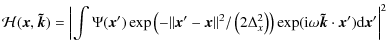
are sought under the assumption that their wavelength is much shorter than the typical lengthscale of the background medium. As discussed by Gough (1993), one expects a better approximation if the starting Eqs. (6)-(8) are first reduced to a so-called normal form that avoids first-order derivatives. This is done in Sect. A.1 leading to
![\begin{displaymath}
\frac{\omega_{\rm c}^2 - \omega^2}{c_{\rm s}^2} \hat{\Psi} +...
..._0} \cdot \vec{\nabla} )\right] \hat{\Psi} = \Delta \hat{\Psi}
\end{displaymath}](/articles/aa/full_html/2009/24/aa11165-08/img49.png)
where
As explained in Sect. A.2, the WKB approximation is then applied to (10). The dominant term of the expansion in powers
of the ratio between the wavelength solution and the background typical lengthscale yields
an equation governing the phase
![]() ,
the so-called eikonal equation.
The amplitude
,
the so-called eikonal equation.
The amplitude
![]() is determined at the next order as a function of
is determined at the next order as a function of
![]() .
By neglecting the gravity waves by taking the high-frequency limit, the eikonal equation reads:
.
By neglecting the gravity waves by taking the high-frequency limit, the eikonal equation reads:

where
In the range of high-frequency acoustic modes, the
2.4 The acoustic ray model as a Hamiltonian system
The acoustic ray model consists in finding solutions to the eikonal Eq. (11) along some path called the ray path.
This problem can be written in a Hamiltonian form
where the solutions
![]() are conjugate variables of the Hamiltonian and t, the parameter
along the path, is a time-like variable.
To derive the Hamiltonian equations from the eikonal equation, one can apply a procedure valid for a general
eikonal equation
are conjugate variables of the Hamiltonian and t, the parameter
along the path, is a time-like variable.
To derive the Hamiltonian equations from the eikonal equation, one can apply a procedure valid for a general
eikonal equation
![]() (e.g. Ott 1993). This leads to the Hamiltonian
(e.g. Ott 1993). This leads to the Hamiltonian
![]() (e.g. Lighthill 1978).
Another useful Hamiltonian formulation can be readily obtained by considering a path normal to the wavefront
(e.g. Lighthill 1978).
Another useful Hamiltonian formulation can be readily obtained by considering a path normal to the wavefront
![]() This method is also used to determine optical rays in isotropic media of variable index (Born 1999), the quantity
This method is also used to determine optical rays in isotropic media of variable index (Born 1999), the quantity
![]() playing
the role of the medium index
playing
the role of the medium index
![]() .
The ray path is thus defined by
.
The ray path is thus defined by
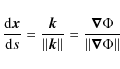
where s is the curvilinear coordinate along the ray. Differenti- ating (13) and using (11) then leads to the following system of ODEs:

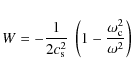
where we use the frequency-scaled wavevector
As W only depends on the spatial variable ![]() ,
the second equation has the classical form of Newton's second law
for the conservative force associated with the potential W(for a unit mass and a time variable t). This system can thus be written in a Hamiltonian form where
,
the second equation has the classical form of Newton's second law
for the conservative force associated with the potential W(for a unit mass and a time variable t). This system can thus be written in a Hamiltonian form where
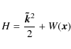
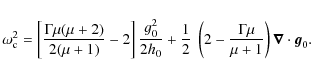
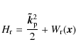
is the Hamiltonian. According to the eikonal Eq. (11), H is equal to zero and the dynamics is therefore fully determined by the potential well W, where frequency
Because the potential is symmetric with respect to the rotation axis of the star, the angular momentum projection on this axis
![]() is a constant of motion, where
is a constant of motion, where
![]() and
and
![]() is a unit vector in the azimuthal direction and
is a unit vector in the azimuthal direction and
![]() are the spherical coordinates.
Consequently, the projection of the ray trajectory on the meridional plane rotating with the ray at an angular velocity
are the spherical coordinates.
Consequently, the projection of the ray trajectory on the meridional plane rotating with the ray at an angular velocity
![]() is governed by the two-degree-of-freedom Hamiltonian:
is governed by the two-degree-of-freedom Hamiltonian:
where
2.5 Numerical method for the ray dynamics
The acoustic ray dynamics has been investigated by integrating numerically Eqs. (14) and (15) using a 5th-order Runge-Kutta method. The step size of the integration is chosen automatically to keep the local error estimate smaller than a given tolerance. To what extent this control of the local error ensures that the numerical solution is close to the true solution depends on the stability of the problem. For chaotic trajectories, the numerical error tends to grow rapidly, while for stable trajectories this error remains of the same order as the relative error. The rapid growth of numerical errors is one of the characteristics of chaotic dynamics; however, this does not prevent simulating such systems since for hyperbolic systems the shadowing theorem (Anosov 1967; Sauer et al. 1997) ensures that an exact trajectory will remain close to the dynamics of each computed point for arbitrary times. Thus while a numerical trajectory diverges from the exact one, it nevertheless remains close to another exact trajectory, and therefore numerical errors do not prevent obtaining accurate phase space plots. We checked that the Poincaré surfaces of section shown in the next section are not significantly modified by decreasing the maximum allowed local error. We also checked the influence of the resolution of the background polytropic stellar model. Increasing this resolution from 62 to 92 Gauss-Lobatto points in the pseudo-radial direction has no significant effect on the Poincaré surface of section. Finally, the Hamiltonian conservation is used as an independent accuracy test of the computation.
3 Acoustic ray dynamics in rotating stars
In this section, we show that rotation strongly modifies the acoustic ray dynamics. Indeed, we find that, as rotation increases, the dynamics undergoes a transition from integrability (at zero rotation) to a mixed state where parts of the phase space display integrable behaviour while other parts are chaotic.
The nature of a dynamical system is best investigated by considering the structure of its phase space which contains both position and momentum coordinates. We thus first introduce the Poincaré surface of section (hereafter the PSS) which is a standard tool to visualize the phase space (Sect. 3.1). Then we describe the phase space structure at zero rotation (Sect. 3.2) and the main features of the generic phase space structure at high rotation rates (Sect. 3.3). The detail of the transition to chaos as rotation increases is analysed in Sect. 3.4. As this last section makes use of several specific tools and theorems of dynamical system theory, it might be skipped at first reading.
3.1 Phase space visualization: the Poincaré surface of section
As shown in Sect. 2.4, acoustic rays with a given Lz are governed by a Hamiltonian with two degrees of freedom ![]() .
The associated phase space is
therefore four-dimensional and difficult to visualize.
A PSS is constructed by computing the intersection of the phase space trajectories
with a chosen (2N-1)-dimensional surface, where N is the number of degrees of freedom of the system.
If H is time-independent, then energy conservation implies that phase space trajectories stay on a (2N-1)-dimensional surface.
The
PSS is thus a (2N-2)-dimensional surface in general and a 2-dimensional surface in the present case.
.
The associated phase space is
therefore four-dimensional and difficult to visualize.
A PSS is constructed by computing the intersection of the phase space trajectories
with a chosen (2N-1)-dimensional surface, where N is the number of degrees of freedom of the system.
If H is time-independent, then energy conservation implies that phase space trajectories stay on a (2N-1)-dimensional surface.
The
PSS is thus a (2N-2)-dimensional surface in general and a 2-dimensional surface in the present case.
![\begin{figure}
\par\includegraphics[width=8cm,clip]{11165fig1.eps}
\end{figure}](/articles/aa/full_html/2009/24/aa11165-08/img91.png) |
Figure 1:
(Colour online) Intersection of an outgoing acoustic ray (red/arrow headed) with the
|
| Open with DEXTER | |
Different choices are possible for the PSS, although some conditions are required to obtain a
good description of the dynamics (see for example Ott 1993).
First, to provide a complete view of phase space, the PSS must be intersected by all phase space trajectories. Here we chose
the curve
![]() situated at a fixed radial distance d from the stellar surface
situated at a fixed radial distance d from the stellar surface
![]() displayed in Fig. 1.
As shown in Sect. B.1
for the non-rotating case,
the distance d can be chosen such that all relevant trajectories intersect this curve.
The second condition is that, given a point on the PSS, the next point on the PSS has to be
uniquely determined. This is ensured by counting the intersection with
displayed in Fig. 1.
As shown in Sect. B.1
for the non-rotating case,
the distance d can be chosen such that all relevant trajectories intersect this curve.
The second condition is that, given a point on the PSS, the next point on the PSS has to be
uniquely determined. This is ensured by counting the intersection with
![]() only when the
trajectory comes from one side of the
only when the
trajectory comes from one side of the
![]() curve. (Here we consider the trajectories coming from the inner side.)
Finally, the coordinate system used to display the PSS is chosen so that any surface of the PSS is conserved by the dynamics in the same way as four-dimensional volumes are preserved in
phase space. The coordinates
curve. (Here we consider the trajectories coming from the inner side.)
Finally, the coordinate system used to display the PSS is chosen so that any surface of the PSS is conserved by the dynamics in the same way as four-dimensional volumes are preserved in
phase space. The coordinates
![]() where
where
![]() is the latitudinal component of
is the latitudinal component of
![]() in the
natural basis
in the
natural basis
![]() associated with the coordinate system
associated with the coordinate system
![]() fulfil this condition (as shown in Sect. B.2).
fulfil this condition (as shown in Sect. B.2).
![\begin{figure}
\par\includegraphics[width=16cm,clip]{11165fig2.eps}
\end{figure}](/articles/aa/full_html/2009/24/aa11165-08/img99.png) |
Figure 2:
(Colour online) PSS at
|
| Open with DEXTER | |
The PSS have been obtained by following many trajectories of different initial conditions.
The number of trajectories, together with the time during which they are computed,
determine the resolution by which the phase space is investigated.
In principle, we should display PSS computed for different values of frequency ![]() .
However, as
.
However, as ![]() is varied in the range of frequency considered here, we found that the PSS remained practically unchanged.
As discussed in Sect. 2.4, this stems from the dynamics of the frequency-scaled wavevector
is varied in the range of frequency considered here, we found that the PSS remained practically unchanged.
As discussed in Sect. 2.4, this stems from the dynamics of the frequency-scaled wavevector
![]() being weakly dependent on
being weakly dependent on ![]() in this frequency range.
in this frequency range.
3.2 The non-rotating case 
The PSS at ![]() is described in this section. It will serve as a reference to
investigate the evolution of the dynamics with rotation.
Due to spherical symmetry, the norm of the angular momentum with respect to the star centre
is described in this section. It will serve as a reference to
investigate the evolution of the dynamics with rotation.
Due to spherical symmetry, the norm of the angular momentum with respect to the star centre
is a conserved quantity. It follows that the intersection of any trajectory with the PSS belongs to a curve of the form
For
The simplicity of the PSS reflects that the system is integrable ((20) indeed provides the second
invariant (in addition to ![]() )
of the reduced two-degree-of-freedom dynamical system).
Every integrable system is structured in N-dimensional surfaces that are associated with specific values
of the N constants of motion. This means that any trajectory is constrained to stay on one of these surfaces forever.
They are called invariant tori because they are invariant through the dynamics and have a torus-like topology.
As we verify in the following,
they play a crucial role in
the transition to chaos, as well as in the mode construction.
The PSS at
)
of the reduced two-degree-of-freedom dynamical system).
Every integrable system is structured in N-dimensional surfaces that are associated with specific values
of the N constants of motion. This means that any trajectory is constrained to stay on one of these surfaces forever.
They are called invariant tori because they are invariant through the dynamics and have a torus-like topology.
As we verify in the following,
they play a crucial role in
the transition to chaos, as well as in the mode construction.
The PSS at ![]() actually visualize the intersection of these tori with the
actually visualize the intersection of these tori with the
![]() surface.
surface.
Important is that the invariant tori can have two different types that determine their fate once the rotation is increased. Rational (or resonant) tori are such that all trajectories on the torus are periodic orbits (i.e. trajectories that close on themselves in phase space). In contrast, irrational tori are such that any trajectory densely covers the whole torus.
3.3 Phase space structure at high rotation rates
The main features of the phase space at high rotation rates are shown in Fig. 2
where the PSS at
![]() is displayed with four acoustic rays shown
on the position space, as well as on the PSS.
These rays belong to the three different types of phase space structures always present at high rotation rates.
First, a large chaotic region appears (the grey region in Fig. 2). Chaotic rays, e.g. the red ray, are not constrained to stay on tori (that is on one-dimensional curves on the PSS) and thus fill up
a phase space volume densely and ergodically (i.e. a surface on the PSS).
Second, the island chain embedded in the large chaotic region is a common structure of phase space at high rotation rate.
An important property of the island chain is to be structured by invariant tori centred on the
periodic orbit of period 2 (the orange ray).
The PSS also shows smaller island chains
like the one formed around a 6-period periodic orbit (see the magenta ray). However, contrary to the 2-period island chain, such
structures survive only up to a certain rotation rate.
Third, the undulated curves present in the high
is displayed with four acoustic rays shown
on the position space, as well as on the PSS.
These rays belong to the three different types of phase space structures always present at high rotation rates.
First, a large chaotic region appears (the grey region in Fig. 2). Chaotic rays, e.g. the red ray, are not constrained to stay on tori (that is on one-dimensional curves on the PSS) and thus fill up
a phase space volume densely and ergodically (i.e. a surface on the PSS).
Second, the island chain embedded in the large chaotic region is a common structure of phase space at high rotation rate.
An important property of the island chain is to be structured by invariant tori centred on the
periodic orbit of period 2 (the orange ray).
The PSS also shows smaller island chains
like the one formed around a 6-period periodic orbit (see the magenta ray). However, contrary to the 2-period island chain, such
structures survive only up to a certain rotation rate.
Third, the undulated curves present in the high
![]() region are formed by whispering gallery type trajectories (like
the green ray),
that is trajectories following the outer boundary. The associated tori correspond to the deformation of non-rotating tori that have not been destroyed
yet at this rotation rate.
Overall this type of phase space organisation is typical of mixed systems
with coexistence of chaotic regions and invariant tori (the structures encountered in integrable systems).
region are formed by whispering gallery type trajectories (like
the green ray),
that is trajectories following the outer boundary. The associated tori correspond to the deformation of non-rotating tori that have not been destroyed
yet at this rotation rate.
Overall this type of phase space organisation is typical of mixed systems
with coexistence of chaotic regions and invariant tori (the structures encountered in integrable systems).
The main phase space structures are dynamically independent since no trajectory can cross from one region to the next. We show in Sect. 4 that the very existence of these structures enables the spectrum to be organised into independent frequency subsets. In the next section, the generic character of these structures is checked by computing the PSS at different rotations.
![\begin{figure}
\par\includegraphics[width=8.5cm,clip]{11165fig3.eps}
\end{figure}](/articles/aa/full_html/2009/24/aa11165-08/img109.png) |
Figure 3:
Three
|
| Open with DEXTER | |
3.4 Transition to chaos

The evolution of the dynamics with increased rotation is first described for
![]() and then for
and then for
![]() .
.
3.4.1 The
 case
case
The PSS computed at the three rotation rates
![]() corresponding to the three flatness
corresponding to the three flatness
![]() are displayed in Fig. 3 to illustrate the effect of a small centrifugal deformation on the ray dynamics.
This perturbation of the integrable
are displayed in Fig. 3 to illustrate the effect of a small centrifugal deformation on the ray dynamics.
This perturbation of the integrable ![]() system is very similar to one described by the KAM-theorem
(Lichtenberg & Lieberman 1992; Lazutkin 1993; Ott 1993; Gutzwiller 1990; Giannoni et al. 1991; Chirikov 1979).
Indeed, for a smooth, small perturbation of an integrable Hamiltonian, this theorem states that the tori of the integrable system that survived
the perturbation occupy most of the phase space volume.
More specifically, while being continuously perturbed, most of the irrational tori can still be associated
with N invariants, thus keeping their torus structure. This is the case for the undulated lines
observed in the high
system is very similar to one described by the KAM-theorem
(Lichtenberg & Lieberman 1992; Lazutkin 1993; Ott 1993; Gutzwiller 1990; Giannoni et al. 1991; Chirikov 1979).
Indeed, for a smooth, small perturbation of an integrable Hamiltonian, this theorem states that the tori of the integrable system that survived
the perturbation occupy most of the phase space volume.
More specifically, while being continuously perturbed, most of the irrational tori can still be associated
with N invariants, thus keeping their torus structure. This is the case for the undulated lines
observed in the high
![]() domain of Fig. 3. In contrast, all rational tori are immediately destroyed for a non-vanishing
perturbation. The KAM theorem implies that, despite the destroyed rational tori forming a dense set in the phase space,
the volume they occupy
vanishes as the perturbation goes to zero.
domain of Fig. 3. In contrast, all rational tori are immediately destroyed for a non-vanishing
perturbation. The KAM theorem implies that, despite the destroyed rational tori forming a dense set in the phase space,
the volume they occupy
vanishes as the perturbation goes to zero.
![\begin{figure}
\par\includegraphics[width=8.5cm,clip]{11165fig4.eps}
\end{figure}](/articles/aa/full_html/2009/24/aa11165-08/img112.png) |
Figure 4:
Three
|
| Open with DEXTER | |
![\begin{figure}
\par\includegraphics[width=8.7cm,clip]{11165fig5.eps}
\end{figure}](/articles/aa/full_html/2009/24/aa11165-08/img114.png) |
Figure 5:
Three
|
| Open with DEXTER | |
The theory of KAM-type transition to chaos also describes how resonant tori disappear.
In our case, they correspond to one-dimensional curves on the PSS,
formed by families of periodic orbits.
All orbits of the same torus will have the same period q.
The so-called Poincaré-Birkhoff
theorem predicts
that a (smooth) small perturbation
will transform this one-dimensional curve into
a chain of q stable points belonging to the same periodic orbit
and surrounded by stable islands, intertwined with q unstable
periodic points. A small chaotic zone appears in the vicinity of the unstable
fixed points and grows with the perturbation. The stable islands have themselves
an intricate self-similar structure of small island chains surrounded by invariant structure (tori).
This phenomenon is illustrated at
![]() in Fig. 3 where, near the
in Fig. 3 where, near the
![]() curve, we can observe
the 2-period island chain around the q=2 stable periodic points
and the small chaotic region around the corresponding unstable points. This results from the destabilization of the
resonant torus associated with the periodic orbits along the diameters of the spherical star.
The widths of the island chains (resonance width)
are expected to be approximately proportional to the square root of the perturbation, and they decrease with q.
curve, we can observe
the 2-period island chain around the q=2 stable periodic points
and the small chaotic region around the corresponding unstable points. This results from the destabilization of the
resonant torus associated with the periodic orbits along the diameters of the spherical star.
The widths of the island chains (resonance width)
are expected to be approximately proportional to the square root of the perturbation, and they decrease with q.
What occurs for large perturbations following the KAM-type transition of integrable Hamiltonians has been studied in many systems.
The general phenomenology that emerges also corresponds to what we observe
in our system
for increased rotation (see the PSS of Fig. 4 computed for
![]() corresponding to the flatness
corresponding to the flatness
![]() ).
The surviving irrational tori, as well as the island chains, are progressively destroyed. This leads to the enlargement of the chaotic regions that were
originally confined by these tori.
This is illustrated in Figs. 3 and 4 where the surface of the central chaotic region becomes progressively larger with rotation.
The island chains typically undergo a series of bifurcations for increasing
perturbation. The most common bifurcation is the period-doubling one,
where a stable periodic orbit of period q is changed to an unstable orbit
plus a stable orbit of period 2q. As the sequence of bifurcations goes on,
stable orbits have longer and longer periods until they eventually disappear.
The destruction of stable regions is
visible between
).
The surviving irrational tori, as well as the island chains, are progressively destroyed. This leads to the enlargement of the chaotic regions that were
originally confined by these tori.
This is illustrated in Figs. 3 and 4 where the surface of the central chaotic region becomes progressively larger with rotation.
The island chains typically undergo a series of bifurcations for increasing
perturbation. The most common bifurcation is the period-doubling one,
where a stable periodic orbit of period q is changed to an unstable orbit
plus a stable orbit of period 2q. As the sequence of bifurcations goes on,
stable orbits have longer and longer periods until they eventually disappear.
The destruction of stable regions is
visible between
![]() and
and
![]() (Fig. 4), as the 6-period island chain embedded in the chaotic central region at
(Fig. 4), as the 6-period island chain embedded in the chaotic central region at
![]() has
disappeared at higher rotation.
As mentioned above, that the largest stable island originates from a short periodic orbit (here a 2-period periodic orbit)
is also a common feature of the KAM-type transitions to chaos.
has
disappeared at higher rotation.
As mentioned above, that the largest stable island originates from a short periodic orbit (here a 2-period periodic orbit)
is also a common feature of the KAM-type transitions to chaos.
While not visible in this figure, a zoom on other regions of the PSS would show the same process going on at small scales.
It is however clear that the irrational tori associated with high values of ![]() survive longer. This property
is also encountered in classical billiards (Lazutkin 1993), where tori
close to the billiard boundary are the most robust.
survive longer. This property
is also encountered in classical billiards (Lazutkin 1993), where tori
close to the billiard boundary are the most robust.
3.4.2 The
 case
case
Qualitatively, the transition to chaos is very similar to the
![]() case. This is shown
in Fig. 5 where PSS computed for
case. This is shown
in Fig. 5 where PSS computed for
![]() are shown for increased rotation.
The main effect of increasing
are shown for increased rotation.
The main effect of increasing
![]() is to delay the transition towards chaos to higher rotation rates.
Indeed by comparing PSS computed at the same rotation rate (see Figs. 4 and
5), one observes that the central chaotic region is
more constrained by surviving tori for higher
is to delay the transition towards chaos to higher rotation rates.
Indeed by comparing PSS computed at the same rotation rate (see Figs. 4 and
5), one observes that the central chaotic region is
more constrained by surviving tori for higher
![]() values. For example
at
values. For example
at
![]() the central chaotic region is much more developed for
the central chaotic region is much more developed for
![]() than for
than for
![]() .
The
.
The
![]() PSS provides another example since for
PSS provides another example since for
![]() the island chain associated with the 6-period orbit
is separated by a surviving KAM tori from the central chaotic
region, while such a stable structure has already been destroyed for
the island chain associated with the 6-period orbit
is separated by a surviving KAM tori from the central chaotic
region, while such a stable structure has already been destroyed for
![]() .
Finally, at
.
Finally, at
![]() ,
we can observe that
the central chaotic region for
,
we can observe that
the central chaotic region for
![]() contains visible surviving structures,
while this is not the case for
contains visible surviving structures,
while this is not the case for
![]() .
.
The slower transition to chaos can be interpreted as caused by the angular constraint
![]() imposed on the dynamics. This is compatible with the trajectories for infinite
imposed on the dynamics. This is compatible with the trajectories for infinite
![]() being confined to the equatorial plane, and the dynamics becoming integrable because of the circular symmetry of this asymptotic limit.
being confined to the equatorial plane, and the dynamics becoming integrable because of the circular symmetry of this asymptotic limit.
4 The asymptotic properties of the acoustic modes
In this section, we show that ray dynamics provides a qualitative and quantitative understanding of the high-frequency acoustic modes. The question to be addressed is how to construct modes, i.e. standing waves, from the short-wavelength propagating waves described by ray dynamics. Such mode construction is expected to be approximately valid in the asymptotic regime of high frequencies. (This asymptotic regime is called the semi-classical regime in a quantum physics context.) As mentioned in the introduction, the answer depends on the nature of the Hamiltonian system. For integrable systems, each phase space trajectory remains on an invariant torus and this enables the construction of modes from a positively interfering superposition of these travelling waves on the torus. This is no longer the case for chaotic systems, where the ray dynamics provides no invariant structures on which to build modes.
Thus for integrable systems, the modes and the frequencies can in principle be explicitly determined from the acoustic rays through well-known formulas called Einstein-Brillouin-Keller (EBK) quantization after the name of its main contributors. We recall the results obtained by Gough (1993) when applying the EBK method to spherical stars (Sect. 4.1). While this procedure is not applicable to chaotic systems, other concepts and methods have been developed and tested in quantum physics to interpret the non-integrable dynamics. These concepts have also been applied to other wave phenomena, such as those observed in e.g. microwave resonators (Stöckmann & Stein 1990), lasing cavities (Nöckel & Stone 1997), quartz blocks (Ellegaard et al. 1996), and underwater waves (Brown et al. 2003). Their potential interest for helioseismology has been suggested, although not demonstrated, by Perdang (1988) and Kosovichev & Perdang (1988). Here, we apply them to the non-integrable ray dynamics of rapidly rotating stars. More specifically, we have seen in Sect. 3 that the ray dynamics of such stars corresponds to a mixed system where parts of phase space display integrable behaviour and other parts chaotic dynamics. In this case, the organisation/classification of modes in the semi-classical regime is expected to closely follow the structure of phase space. Near-integrable regions of phase space like the island chains are amenable to EBK quantization, leading to a regular frequency spectrum, while the modes originating in chaotic regions have an irregular frequency spectrum with generic statistical properties. Another important information provided by ray dynamics is the averaged number of modes that can be constructed from a given phase space region. This number is proportional to the volume of the region considered.
In the following, we explain these concepts and methods in the context of stellar
acoustics (Sects. 4.1-4.3).
Then, their relevance in describing the asymptotic properties of the acoustic modes is tested
by comparing their predictions to the actual
properties of
high-frequency
acoustic modes (Sects. 4.4-4.7).
These modes are axisymmetric modes in the
frequency range
![]() ,
,
![]() being the lowest acoustic mode frequency of the stellar model considered.
They were computed for a
being the lowest acoustic mode frequency of the stellar model considered.
They were computed for a
![]() uniformly rotating
uniformly rotating ![]() polytropic model of star and under the same assumptions
as for ray dynamics (adiabatic perturbations, no Coriolis acceleration, Cowling approximation).
polytropic model of star and under the same assumptions
as for ray dynamics (adiabatic perturbations, no Coriolis acceleration, Cowling approximation).
4.1 The integrable case
To build modes from the ray dynamics, the
wave-like solution
![]() is regarded as a function of the phase space variables
is regarded as a function of the phase space variables
![]() that is subsequently projected onto the position space.
The condition that
that is subsequently projected onto the position space.
The condition that
![]() be single-valued on the position space requires that, for any phase space trajectory that closes on itself
in the position
space, the variation in
be single-valued on the position space requires that, for any phase space trajectory that closes on itself
in the position
space, the variation in ![]() along this closed contour is a multiple of
along this closed contour is a multiple of ![]() .
As trajectories of an integrable system stay on invariant tori,
this condition leads to the EBK formula
.
As trajectories of an integrable system stay on invariant tori,
this condition leads to the EBK formula
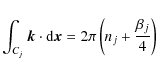
where Cj is any closed contour on a given torus and nj and
While this expression is valid for any closed contour on the torus, it can be shown
that it gives the same condition for all
contours that can be continuously deformed to the same one.
Thus
in fact the EBK quantization yields N independent conditions, as only Ntopologically independent closed paths exist on an N-dimensional torus. As these closed paths
do not need to
be actual trajectories of the dynamical system,
the
usual way to construct EBK solutions is to choose contours for which the formulas are simple to compute.
The quantization conditions thus
select a particular torus on which a mode can be
built, irrespective of whether the torus is resonant or non-resonant.
For spherical stars, three independent contours on a torus specified by L, Lz and ![]() can be obtained by varying one of the
spherical coordinates and fixing the other two. Using similar contours, Gough (1993) obtained the three conditions:
can be obtained by varying one of the
spherical coordinates and fixing the other two. Using similar contours, Gough (1993) obtained the three conditions:
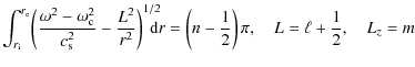
where n,
The tori on which the eigenmodes are constructed can be visualized on the PSS.
For example, the
![]() mode is associated
with the torus
mode is associated
with the torus
![]() ,
,
![]() and its imprint on the PSS are the straight lines
and its imprint on the PSS are the straight lines
![]() .
The intersection of various mode-carrying tori with the
.
The intersection of various mode-carrying tori with the
![]() PSS are shown in Fig. 3. High radial order modes approach the central
PSS are shown in Fig. 3. High radial order modes approach the central
![]() line, while high-degree modes
occupy the high
line, while high-degree modes
occupy the high
![]() region.
region.
4.2 Chaotic systems
It has been widely recognised in the past few decades that most dynamical systems are not integrable and therefore display various degrees of chaos. The quantum chaos field has studied quantum systems whose short-wavelength classical limit displays such chaotic behaviour. As recognised early by Einstein (1917), the EBK quantization explained in the above paragraph cannot be applied to these systems. Indeed, no N-dimensional invariant structure exists on which to apply conditions of constructive interference like the EBK condition. Rather, the semi-classical limit of these chaotic systems yields a Fourier-like formula that connects the set of all classical periodic orbits to the whole spectrum. This formula, called the Gutzwiller trace formula (Gutzwiller 1990) is much more delicate to use than EBK formulas, since it represents a divergent sum from which information can only be extracted through refined mathematical and numerical methods.
On the other hand, the very complexity of chaotic systems leads to statistical universalities. Indeed, in a similar way as statistical physics emerges from the random behaviour of individual particles, in chaotic systems the randomness induced by chaos leads to robust statistical properties of eigenmodes. In contrary to modes of integrable systems, which are localized on individual tori selected by the EBK conditions, in chaotic systems modes are generally not associated to a specific structure in phase space and are ergodic on the energy surface. It has been found that one can model such systems by replacing the Hamiltonian by a matrix whose entries are random variables with Gaussian distributions. Such ensembles of random matrices, which contain no free parameter but take the symmetries of the system into account, can give precise predictions, which have been found to accurately describe many statistical properties of the modes of systems with a chaotic classical limit. This has been conjectured and checked numerically for many systems (Bohigas et al. 1984; Giannoni et al. 1991).
The comparison with the predictions of the Random Matrix Theory (hereafter the RMT)
is often done through the statistical analysis of the frequency spectrum.
In general
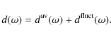
the density of modes as a function of the frequency
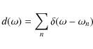 |
(24) |
where
The quantity
The spectra of integrable systems are
predicted to be uncorrelated, and in general this leads to fluctuations
given by the Poisson distribution (Berry & Tabor 1977). In contrast,
for chaotic systems these fluctuations should be given by the RMT.
The RMT
has therefore been developed to analytically compute
the predictions for specific quantities, which in turn could be compared
to numerical data for real systems. A popular quantity to describe
fluctuations in spectra is the spacing distribution ![]() ,
which
is the distribution of spacings in frequency between consecutive eigenfrequencies,
once the frequency differences have been rescaled by
the Weyl term such that the average spacing is one.
The function
,
which
is the distribution of spacings in frequency between consecutive eigenfrequencies,
once the frequency differences have been rescaled by
the Weyl term such that the average spacing is one.
The function ![]() measures the correlations at
short distances in frequency in the spectrum. It does not give
information
about all statistical properties, but it is nevertheless very useful
since the predictions are
strikingly different for the Poisson distribution and for the RMT.
While the Poisson distribution corresponds to
measures the correlations at
short distances in frequency in the spectrum. It does not give
information
about all statistical properties, but it is nevertheless very useful
since the predictions are
strikingly different for the Poisson distribution and for the RMT.
While the Poisson distribution corresponds to
![]() ,
the prediction of the RMT is the Wigner
distribution
,
the prediction of the RMT is the Wigner
distribution
![]() ,
which displays frequency
repulsion (level repulsion in the quantum terminology) at short
distances (small
,
which displays frequency
repulsion (level repulsion in the quantum terminology) at short
distances (small ![]() )
and falls off faster than Poisson at large
)
and falls off faster than Poisson at large ![]() .
.
4.3 Mixed systems
We have seen in Sect. 3 that the acoustic ray dynamics in rotating stars has a mixed character as chaotic regions coexist with stables structures like island chains or invariant tori. Such mixed systems are actually the most common in nature, completely integrable and chaotic systems being limiting cases.
In the context of quantum chaos, seminal studies of these systems by Percival (1973) and Berry & Robnik (1984) led to conjecture that a good description of their spectrum at high energy is obtained by quantizing the structured and chaotic parts independently. While a zoom on island regions would reveal a complex structure involving chaotic trajectories and chains of smaller islands, these small scale details can be neglected for the island quantization if the mode wavelength remains larger than these scales. Instead, the presence of a large number of invariant structures constrains enough the dynamics to make the system similar to a purely integrable structure to which EBK quantization applies. These region are then called near-integrable.
Subsets of modes can be associated to the different near-integrable island chains, while other subsets correspond to the chaotic zones. In each subset, the modes behave as if they were constructed from an isolated system; thus, in mixed systems the frequency spectrum can be described as a superposition of independent frequency subsets associated with the different phase space regions. Subsequent works have shown this picture to be a good approximation of actual spectra, although in some cases certain correlations are present between the frequency subsets due to the presence of partial barriers in phase space or to the existence of modes localized at the border between zones (Bohigas et al. 1993).
Because the acoustic ray dynamics of rapidly rotating stars is of this mixed type, one can expect such an organisation of the spectrum to be valid, even though the modes have quite long wavelength compared to previous studies in quantum chaos. To test this hypothesis, it is convenient to compute a phase-space representation of the modes. Indeed, the chaotic or near-integrable zones are well-defined in phase space, while their projections in position space, where modes are usually pictured, are generally much more difficult to separate.
4.4 Associating modes to rays
Constructing phase space representations for
modes has been envisioned since the beginning
of quantum mechanics, since it enables testing the
quantum-classical correspondence accurately.
In contrast to states of a classical system, which are defined by a point in phase space, modes have always a finite extension in phase space
since they have a finite wavelength and their localization in wavenumber space
is, according to Fourier
analysis, inversely
proportional to their localization in physical space.
Any mode occupies a finite volume of the order of ![]() in the physical/wavenumber phase space
(a
in the physical/wavenumber phase space
(a
![]() volume in the physical/scaled-wavenumber (
volume in the physical/scaled-wavenumber (![]() ,
,
![]() )
phase space or
a
)
phase space or
a
![]() volume in the position/momentum phase space of quantum physics).
Wigner (1932) was the first to construct a phase space function representing
a mode, but this so-called Wigner function
has the disadvantage of being positive or negative, and so
cannot be interpreted as a probability distribution of the
mode.
To circumvent this problem, one way is to smooth the Wigner
function by a Gaussian convolution. The resulting function, called
the Husimi distribution function (Chang & Shi 1986), is always real and nonnegative and
can be equally understood
as the projection of the mode onto
a Gaussian wave packet centred on
volume in the position/momentum phase space of quantum physics).
Wigner (1932) was the first to construct a phase space function representing
a mode, but this so-called Wigner function
has the disadvantage of being positive or negative, and so
cannot be interpreted as a probability distribution of the
mode.
To circumvent this problem, one way is to smooth the Wigner
function by a Gaussian convolution. The resulting function, called
the Husimi distribution function (Chang & Shi 1986), is always real and nonnegative and
can be equally understood
as the projection of the mode onto
a Gaussian wave packet centred on ![]() and
and
![]() :
:
where
![]() is the mode and
is the mode and
![]() the Gaussian
wavepacket.
In this expression,
the width
of the wavepacket
the Gaussian
wavepacket.
In this expression,
the width
of the wavepacket ![]() determines the resolution of the Husimi function in the spatial direction, the resolution in the scaled-wavenumber
determines the resolution of the Husimi function in the spatial direction, the resolution in the scaled-wavenumber
![]() being such that
being such that
![]() .
These quantities determine the minimal extent of the mode representation in both directions.
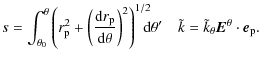
.
These quantities determine the minimal extent of the mode representation in both directions.
The computed modes are 3D modes and they shall be compared with the reduced ray dynamics computed
on a 2D meridional plane. As shown in the spherical case by Gough (1993), the amplitude of a 3D axisymmetric mode constructed
from acoustic rays obtained on neighbouring
meridional planes decreases as
![]() because
the distance between the planes and thus
the density of rays increases away from the rotation axis.
Thus, the computed 3D modes were scaled by
because
the distance between the planes and thus
the density of rays increases away from the rotation axis.
Thus, the computed 3D modes were scaled by
![]() to better
represent the mode amplitude on a meridional plane.
Moreover, to obtain a phase-space representation limited to the PSS, we
actually computed the Husimi's distribution function of the
1D cut of the mode taken along the PSS:
to better
represent the mode amplitude on a meridional plane.
Moreover, to obtain a phase-space representation limited to the PSS, we
actually computed the Husimi's distribution function of the
1D cut of the mode taken along the PSS:
where
The vector
![\begin{figure}
\par\includegraphics[width=8cm,clip]{11165fig6.eps}
\end{figure}](/articles/aa/full_html/2009/24/aa11165-08/img170.png) |
Figure 6:
(Colour online) Four axisymmetric modes and their phase space representation: a) a 2-period island mode (blue/dark grey),
b) a chaotic mode (red/grey), c) a 6-period island mode (magenta/light grey), and d) a whispering gallery
mode (green/light grey). The amplitude distribution of the
scaled mode |
| Open with DEXTER | |
The Husimi function has been computed for the axi-symmetric modes of the
![]() star,
and its contour plot is compared with the PSS of the ray dynamics computed for the same star model.
Figure 6 illustrates this process by showing the position space, as well as the phase space
representation of four typical modes.
As can be observed, the modes can be clearly associated with one of the main
structures of the phase space, namely, the 2-period island chain, the large central chaotic region,
the 6-period island chain or the whispering gallery region.
On the PSS, we note, however, that the Husimi function is symmetric with respect to
star,
and its contour plot is compared with the PSS of the ray dynamics computed for the same star model.
Figure 6 illustrates this process by showing the position space, as well as the phase space
representation of four typical modes.
As can be observed, the modes can be clearly associated with one of the main
structures of the phase space, namely, the 2-period island chain, the large central chaotic region,
the 6-period island chain or the whispering gallery region.
On the PSS, we note, however, that the Husimi function is symmetric with respect to
![]() while the dynamics is not.
This difference stems from the PSS being only constructed with
while the dynamics is not.
This difference stems from the PSS being only constructed with
![]() intersecting trajectories,
while the Husimi function computed from the
mode cut on the
intersecting trajectories,
while the Husimi function computed from the
mode cut on the
![]() contains no information about the sign of
contains no information about the sign of
![]() .
Nevertheless, in the high-frequency interval
.
Nevertheless, in the high-frequency interval
![]() that we studied in detail,
any ambiguity on the phase space location can always be resolved using the additional information
on the mode distribution in the position space.
In this frequency interval, we thus classified the modes according to their localization in phase space
distinguishing the 2-period island modes, the chaotic modes, the 6-period island modes
and the whispering gallery modes associated with the corresponding phase space regions.
As a result, the full frequency spectrum can be decomposed into subspectra associated with phase space structures.
Figure 7 displays the four subspectra.
that we studied in detail,
any ambiguity on the phase space location can always be resolved using the additional information
on the mode distribution in the position space.
In this frequency interval, we thus classified the modes according to their localization in phase space
distinguishing the 2-period island modes, the chaotic modes, the 6-period island modes
and the whispering gallery modes associated with the corresponding phase space regions.
As a result, the full frequency spectrum can be decomposed into subspectra associated with phase space structures.
Figure 7 displays the four subspectra.
![\begin{figure}
\par\includegraphics[width=9cm,clip]{11165fig7.eps}
\end{figure}](/articles/aa/full_html/2009/24/aa11165-08/img173.png) |
Figure 7: Frequency subspectra of four classes of axisymmetric modes: a) the 2-period island modes, b) the chaotic modes antisymmetric with respect to the equator, c) the 6-period island modes, and d) some whispering gallery modes. For the subspectra a) and d), the height of the vertical bar specifies one of the two quantum numbers characterising the mode. |
| Open with DEXTER | |
In the following, we analyse these subspectra and test whether the Percival and Berry-Robnik conjecture described in Sect. 4.3 applies to acoustic modes in rapidly rotating stars. We first study the regular character of the subspectra issued from near-integrable phase space regions (Sect. 4.5) and then consider the spectrum of chaotic modes (Sect. 4.6).
4.5 The regular spectra
A spectrum is said to be regular if it can
be described by a function of N integers, N being the degree of freedom of the system.
In accordance with previous studies by Lignières et al. (2006), Lignières & Georgeot (2008), and Reese et al. (2008), the spectrum
of the 2-period island modes
is well-fitted by the empirical
formula
confirming the regular nature of this spectrum that is also clearly apparent in Fig. 7a.
The 6-period island mode spectrum shown in Fig. 7c is also regular, since it is closely fitted by the even simpler formula
Indeed, the root mean square error between this empirical fit and the actual spectrum is equal to 1.9 percent of
While a simple linear law, such as Eqs. (29) or (30), does not apply to the whispering gallery modes, there is strong evidence that this subspectrum is also regular. Thanks to the regularity of the nodal lines pattern (as apparent in Fig. 6d), two integers corresponding to the number of nodes along the polar axis and to the number of nodes following the internal caustic can be easily attributed to each mode. When plotted against the number of caustic nodes (as in Fig. 7d), the spectrum clearly shows a regular behaviour. That the function of these two integers describing the spectrum is not as simple as Eqs. (29) or (30) is expected from what we know about the regular spectrum of high-degree modes in spherical stars (see for example Christensen-Dalsgaard 1980).
The regularity of the three subspectra issued from near-integrable phase space regions
is fully in accordance with the Percival's conjecture.
An important consequence is that the theoretical model of these spectra can in principle
be obtained from the EBK quantization
of the invariant structures of the corresponding near-integrable regions.
As a result we should be able to
relate the potentially
observable quantities
![]() ,
,
![]() ,
or
,
or
![]() to the star properties.
In practice, the standard method is first to construct
the normal forms around the central periodic orbit in order to describe
the dynamics in the island, and then use the EBK
quantization scheme to find the asymptotic formula for the modes
(Lazutkin 1993; Bohigas et al. 1993).
While such a programme is outside the scope of the present paper, we mention below the result
obtained in Lignières & Georgeot (2008) for the 2-period island modes using an
equivalent procedure, which may be more physically transparent, and extend it to the 6-period island modes.
to the star properties.
In practice, the standard method is first to construct
the normal forms around the central periodic orbit in order to describe
the dynamics in the island, and then use the EBK
quantization scheme to find the asymptotic formula for the modes
(Lazutkin 1993; Bohigas et al. 1993).
While such a programme is outside the scope of the present paper, we mention below the result
obtained in Lignières & Georgeot (2008) for the 2-period island modes using an
equivalent procedure, which may be more physically transparent, and extend it to the 6-period island modes.
As already noted, the propagation of acoustic waves in
our system is similar to the propagation of light in an inhomogeneous
medium, where the role of the medium index is played by
![]() .
The construction of standing-wave
solutions between two bounding surfaces has
been investigated intensively in the context
of the study of laser modes in cavities (Kogelnik & Li 1966) and consists
in applying the paraxial approximation in the vicinity
of the optical axis. While generally applied to homogeneous media, this approximation can be extended to the inhomogeneous case as in Bornatici & Maj (2003); Permitin & Smirnov (1996). Applying this formalism to the acoustic modes
associated with periodic orbits,
Lignières & Georgeot (2008) found a model spectrum equivalent to Eq. (29) with
.
The construction of standing-wave
solutions between two bounding surfaces has
been investigated intensively in the context
of the study of laser modes in cavities (Kogelnik & Li 1966) and consists
in applying the paraxial approximation in the vicinity
of the optical axis. While generally applied to homogeneous media, this approximation can be extended to the inhomogeneous case as in Bornatici & Maj (2003); Permitin & Smirnov (1996). Applying this formalism to the acoustic modes
associated with periodic orbits,
Lignières & Georgeot (2008) found a model spectrum equivalent to Eq. (29) with
where
The 6-period island mode spectrum can be modelled in the same way. In the frequency
interval considered, these modes
have a similar structure in the direction transverse to the central orbit and should therefore be
associated with the same ![]() value.
The model spectrum has thus the same form as Eq. (30) where
value.
The model spectrum has thus the same form as Eq. (30) where

As for the 2-period modes, we find that this theoretical value of
These two examples show that ray dynamics can provide a quite accurate model of the near-integrable spectra in the relatively low-frequency regime considered here. Moreover, model (29) of the 2-period island mode spectrum remains reasonably accurate at lower frequencies (Lignières et al. 2006) and can be extended to non-axisymmetric modes (Reese et al. 2008).
4.6 The chaotic modes
A large subset of the frequencies correspond
to modes localized in the chaotic zone of phase space (the chaotic modes). As we have seen
in Sect. 4.2, one should not expect regular patterns for this part of the
spectrum. Rather, the chaotic character of the phase space should be reflected
in specific statistical properties of the subspectrum, which should follow
predictions from Random Matrix Theory. To test this predictions, we
have studied the distribution of the consecutive frequency spacings
![]() of the chaotic modes.
Figure 8 shows the integrated
distribution
of the chaotic modes.
Figure 8 shows the integrated
distribution
![]() (with spacings normalized by the mean
level spacing within the chaotic subset, as should be done).
The distribution is constructed from the two independent distributions obtained for
the equatorially symmetric and anti-symmetric modes, corresponding to around 187 modes in total.
Although the difficulty of solving Eqs. (6)-(8) prevents us from reaching
such large frequency samples as can be obtained for other systems (Bohigas et al. 1984),
the numerically computed
(with spacings normalized by the mean
level spacing within the chaotic subset, as should be done).
The distribution is constructed from the two independent distributions obtained for
the equatorially symmetric and anti-symmetric modes, corresponding to around 187 modes in total.
Although the difficulty of solving Eqs. (6)-(8) prevents us from reaching
such large frequency samples as can be obtained for other systems (Bohigas et al. 1984),
the numerically computed ![]() agrees well with the RMT predictions,
and is clearly different from the Poisson distribution typical of
integrable systems. This result indicates that these modes, selected
by the comparison between their localization in phase space and
the ray dynamics, indeed have the frequency statistics expected for chaotic
modes.
We therefore think that this validates the ray model,
and gives strong evidence that wave chaos actually
occurs in rapidly rotating stars.
agrees well with the RMT predictions,
and is clearly different from the Poisson distribution typical of
integrable systems. This result indicates that these modes, selected
by the comparison between their localization in phase space and
the ray dynamics, indeed have the frequency statistics expected for chaotic
modes.
We therefore think that this validates the ray model,
and gives strong evidence that wave chaos actually
occurs in rapidly rotating stars.
| |
Figure 8:
Integrated spacing distribution |
| Open with DEXTER | |
The modes we identify as chaotic are located in the chaotic zone but cover only part of it, as for the example of Fig. 6. We think this is partly due to the relatively low frequency considered, which prevents the ergodicity of the modes from being clearly visible. In addition, it is known that certain low-energy eigenfunctions of chaotic systems called scars are concentrated along short periodic orbits of the system (Heller 1984). In this case, rather than being ergodic, some individual modes are effectively localized in the vicinity of such orbits. This effect can create some subsequences of low-energy modes with regular frequency patterns, even if the distribution of frequency spacings follows the predictions of the RMT. Precise investigation of this phenomenon in the context of stellar acoustic modes may be important.
4.7 Predicting the number of modes in each subspectrum: the Weyl formula
In this section, we show that ray dynamics enables an estimate of the number of chaotic and island modes present within a given frequency interval. This information is complementary to the regular/irregular properties of the associated subspectra shown in the previous section and it is crucial to building an asymptotic model of the frequency spectrum.
We have seen in Sect. 4.2 that the density of modes as a function of the frequency
![]() can be written as the sum of a smooth part
can be written as the sum of a smooth part
![]() and
an oscillatory part
and
an oscillatory part
![]() (see Eq. (25)).
At the beginning of the twentieth century, Weyl analytically derived an asymptotic expansion of
(see Eq. (25)).
At the beginning of the twentieth century, Weyl analytically derived an asymptotic expansion of
![]() (Weyl 1912).
The leading term of the Weyl formula can be obtained from
general principles.
We have seen (Sect. 4.4) that in average a mode occupies a
(Weyl 1912).
The leading term of the Weyl formula can be obtained from
general principles.
We have seen (Sect. 4.4) that in average a mode occupies a ![]() volume
in the physical/wavenumber phase space.
The averaged number
of modes in a given phase space volume can thus be estimated as the volume of phase space
available divided by
volume
in the physical/wavenumber phase space.
The averaged number
of modes in a given phase space volume can thus be estimated as the volume of phase space
available divided by ![]() ,
the volume occupied by one mode.
In the following, we first verify that the leading term of the Weyl formula
yields a reasonable estimate of the number of modes in the case of spherically symmetric stars.
Then, we calculate the phase space volume of the chaotic and island regions
and confront the result with those obtained from the numerical computation of modes at
,
the volume occupied by one mode.
In the following, we first verify that the leading term of the Weyl formula
yields a reasonable estimate of the number of modes in the case of spherically symmetric stars.
Then, we calculate the phase space volume of the chaotic and island regions
and confront the result with those obtained from the numerical computation of modes at
![]() .
.
The Hamiltonian formulation
![]() is best suited
to this calculation. The averaged
number of modes below a given frequency
is best suited
to this calculation. The averaged
number of modes below a given frequency ![]() reads as
reads as
where
where
For spherical stars, the dynamics can be reduced to the
one-degree-of-freedom dynamics characterised by the reduced Hamiltonian
![]() .
Applying the above formula to
.
Applying the above formula to
![]() ,
the double integral
,
the double integral
![]() can be integrated over
can be integrated over ![]() to give
to give
 |
(35) |
which is thus the estimated number of modes of given L and Lz with a frequency lower than
In rotating stars, to estimate
![]() the number of modes below
the number of modes below ![]() for a given Lz, we use
the two-degree-of-freedom Hamiltonian
for a given Lz, we use
the two-degree-of-freedom Hamiltonian
![]() ,
and integrate the 4-dimensional volume integral in the wavenumber directions to obtain
,
and integrate the 4-dimensional volume integral in the wavenumber directions to obtain
 |
(36) |
where
The 4-dimensional phase space volumes were evaluated using a Monte-Carlo quadrature method: points are randomly
chosen in a known volume ![]() that includes the volume V to be computed. The proportion of points
inside V approximates the ratio
that includes the volume V to be computed. The proportion of points
inside V approximates the ratio
![]() ,
thus providing an approximate value of V.
To decide
whether a given point
is inside or outside V, we used
space-filling trajectories on the torus delimiting the volume V.
Two phase space volumes were computed at
,
thus providing an approximate value of V.
To decide
whether a given point
is inside or outside V, we used
space-filling trajectories on the torus delimiting the volume V.
Two phase space volumes were computed at
![]() .
The first one
includes the large chaotic region, as well as the island chains around the 2-period and 6-period orbits.
The second volume corresponds to the 2-period island chain.
The details of the calculation and an estimation of the error on the volume determination are given in Sect. C.
.
The first one
includes the large chaotic region, as well as the island chains around the 2-period and 6-period orbits.
The second volume corresponds to the 2-period island chain.
The details of the calculation and an estimation of the error on the volume determination are given in Sect. C.
As a result, the leading term of the Weyl formula yields ![]() modes in the 2-period island chain
and
modes in the 2-period island chain
and ![]() modes outside the whispering gallery region in the frequency interval
modes outside the whispering gallery region in the frequency interval
![]() .
This value has to be compared with the 50 island modes and the 276 modes outside the whispering gallery region
obtained using the Husimi phase space representation of the modes computed in the same frequency interval.
.
This value has to be compared with the 50 island modes and the 276 modes outside the whispering gallery region
obtained using the Husimi phase space representation of the modes computed in the same frequency interval.
The difference between the estimation given by (33) and the actual number of modes in each subset of the frequency spectrum most likely corresponds to the next order in the asymptotic expansion of the density of modes. Indeed, Eq. (33) is only the first term in an asymptotic expansion, the next term usually being proportional to the length of the boundary between phase space zones. At relatively low frequency, this term can be significant. Another source of imprecision can stem from how, at such relatively low frequency, some partial barriers in phase space can trap island-like modes in the vicinity of the island, enlarging the effective size of the regular zone. Indeed, for some of the modes classified as island modes, the Husimi distribution is not entirely inside the island, the outer part remaining close to the island. Nevertheless, our study shows that Eq. (33) gives a reliable estimate of the relative sizes of the frequency subsets that can be obtained without any knowledge of the spectrum itself.
5 Discussion and applications to asteroseismology
In this section we discuss the validity of the assumptions of our asymptotic analysis and the implications of our results for the asteroseismology of rapidly rotating stars.
5.1 Assumptions of the asymptotic analysis
The WKB assumption underlying the asymptotic analysis is not justified for the lowest frequency acoustic modes. While determining the limit of validity of the different results presented here is outside the scope of the paper, we know that the regularities of the 2-period island mode subspectrum are relevant down to about the 5th radial order acoustic pulsations (see Lignières et al. 2006; and Reese et al. 2008, for details).
Another important precaution when applying the present analysis stems from
the interpretation of the ray dynamics depending on the frequency range considered.
Indeed, if extremely high-frequency modes were to exist,
their properties would closely follow the phase space structure up to its smallest details.
This means, for example, that such modes could be associated with the very small chaotic regions
that exist inside the island chains or in between the surviving KAM tori of the whispering gallery regions.
On the other hand,
finite-wavelength effects have to be taken into account when interpreting the ray dynamics at finite frequencies.
For example, the regularities of the island mode spectra in the
![]() interval show
that the small chaotic zones within the island chain can be overlooked in this frequency range.
The same reasoning holds if one wants to interpret the ray dynamics at small rotation rates (see Fig. 3).
The tiny chaotic regions predicted
by the KAM theorem could be interpreted as a proof for the existence of a chaotic mode frequency subset at vanishingly small rotation.
However, these modes should have such a short wavelength to ``fit in'' the chaotic region
that they may simply not exist (because they are strongly dissipated by diffusive effects
or their frequency is so high that they are not reflected at the surface).
interval show
that the small chaotic zones within the island chain can be overlooked in this frequency range.
The same reasoning holds if one wants to interpret the ray dynamics at small rotation rates (see Fig. 3).
The tiny chaotic regions predicted
by the KAM theorem could be interpreted as a proof for the existence of a chaotic mode frequency subset at vanishingly small rotation.
However, these modes should have such a short wavelength to ``fit in'' the chaotic region
that they may simply not exist (because they are strongly dissipated by diffusive effects
or their frequency is so high that they are not reflected at the surface).
Ray dynamics cannot directly account directly for the coupling effects between two modes associated with two dynamically isolated regions of phase space (as occurs for example in the well known tunneling effect). Indeed, while trajectories cannot cross the dynamical barrier between the chaotic and the island chain regions, an island mode can be present on either side of the barrier if its frequency is very close to the one of a chaotic mode (and vice versa). As usual for mode avoided crossings, the mode distribution can thus be significantly perturbed by the coupling, but the frequency is only slightly affected especially in the high-frequency regime. Quantifying the effects of such avoided crossings would require a specific study.
The WKB assumption that the wavelength is much shorter than the typical background lengthscale breaks down for low-frequency acoustic mode but also when the typical lengthscale of the stellar model becomes very small. This can occur in real stars, especially at the upper limit of the core convective zone where strong composition gradients build in during evolution. The effect of such a discontinuity has been studied for spherical stars (Ballot et al. 2004; Gough 1990; Vorontsov 1988) and has been found to add an oscillatory component to Tassoul's asymptotic formula, but not to remove the asymptotic structure altogether. To treat the discontinuities properly in non-spherical stars, the ray dynamics approach has to be extended by taking into account the splitting of rays at the discontinuity, corresponding to the reflected and transmitted waves. Once this is incorporated in the formalism, quantum chaos techniques can be applied as done for billiards in Bluemel et al. (1996a,b), and the Weyl formula can also be computed (Prange et al. 1996).
Apart from the treatment of eventual sound-speed discontinuities, the asymptotic analysis presented in this paper for uniformly rotating polytropic stellar models can be readily applied to realistic stellar models. The details of the dynamics will change because they depend on the sound speed distribution of the model considered. However, we do not expect that the mixed character of the dynamics and thus the irregular/regular nature of the spectrum will change. This has to be confirmed by specific ray dynamics studies. In particular, the effects of the advection by a differentially rotating flow should be investigated.
Lifting the two assumptions concerning the adiabaticity of the perturbations and the Coriolis force omission should not significantly modify the results of the asymptotic analysis. Non-adiabatic calculations are known to have a small effect on the frequency values, while the legitimate omission of the Coriolis force for high-frequency motions is already relevant for quite low frequency as shown in Reese et al. (2006).
5.2 Implications for mode identification
The asymptotic analysis provides qualitative and quantitative information that can be used
to identify high-frequency acoustic modes in an observed spectrum.
First the basic structure of the spectrum can be readily deduced from the ray dynamics phase space structure visualized by the PSS.
Indeed, we have seen that the
![]() PSS
correctly predicts that
the spectrum of axi-symmetric modes is a superposition of four frequency subsets, three regular and one irregular.
If we now look at the
PSS
correctly predicts that
the spectrum of axi-symmetric modes is a superposition of four frequency subsets, three regular and one irregular.
If we now look at the
![]() PSS, we see that the spectrum structure should be similar except that
the regular subspectrum associated with the 6-period island chain is no longer present
since this island chain has disappeared at this rotation rate.
In the same way, at
PSS, we see that the spectrum structure should be similar except that
the regular subspectrum associated with the 6-period island chain is no longer present
since this island chain has disappeared at this rotation rate.
In the same way, at
![]() ,
we expect a simple superposition of a whispering gallery subspectrum
and a 2-period island mode subspectrum since the chaotic regions are not developed enough at this rotation rate.
Such information, while only qualitative, is crucial for guiding the identification process.
Moreover this information is obtained at relatively low computing cost since the PSS calculation is much less demanding
than the numerical computation of modes and frequencies.
,
we expect a simple superposition of a whispering gallery subspectrum
and a 2-period island mode subspectrum since the chaotic regions are not developed enough at this rotation rate.
Such information, while only qualitative, is crucial for guiding the identification process.
Moreover this information is obtained at relatively low computing cost since the PSS calculation is much less demanding
than the numerical computation of modes and frequencies.
Then, the EBK quantization of the near-integrable regions provides the values of the uniform frequency spacings (as given by Eq. (29)) that should be present in the observed spectrum. When analysing an observed spectrum, the star model is not known, so that only estimates of these uniform spacings can be obtained. However, these estimates enable to focus the search for regularities on a narrower range of values.
Finally as we also know the frequency statistics of chaotic modes and the number of modes in each subspectrum (through Weyl's formula), the asymptotic analysis enables construction of asymptotic spectra. The chaotic mode frequencies can be obtained as a realization of the Wigner distribution, although in this case, their frequencies could not be individually identified with observed ones. Nevertheless, such a synthetic spectrum should be very useful when testing identification methods, especially the search for the regularities hidden in the complete spectrum (see below).
Among the additional information that can help constraint the mode identification are the mode visibility and the mode excitation.
The excitation mechanism has been studied so far in the spherically symmetric case and needs to be reconsidered for rapidly rotating stars.
The mode visibility also deserves specific study, notably the calculation of
the intensity variations induced by the oscillation in a gravity darkened atmosphere.
However, the visibility strongly depends on the cancellation effects on the disk-integrated light.
Here, we can estimate this effect by integrating the surface Lagrangian temperature perturbation of the axisymmetric modes
computed for the
![]() rotating polytropic star.
The disk-averaging factor is defined as
rotating polytropic star.
The disk-averaging factor is defined as
where i is the inclination angle between the line-of-sight and the rotation axis,
and the projected visible surface is normalized by
![\begin{figure}
\par\includegraphics[width=9cm,clip]{11165fig9.eps}
\end{figure}](/articles/aa/full_html/2009/24/aa11165-08/img220.png) |
Figure 9:
(Colour online) Frequency spectra of axisymmetric modes where the amplitude is given by the normalized disk-averaging factor D(i) for
a star seen pole-on i =0 and equator-on |
| Open with DEXTER | |
Figure 9 shows the spectrum of axisymmetric modes whose disk-averaging factor exceeds 2.5 percent.
It appears that the disk-averaging effect does not allow to discard as many modes as for spherical stars.
Indeed, in a given frequency interval and for the same visibility threshold, we find that the number of visible modes is more than three
time higher in the
![]() star than in a spherical star.
Among the four classes of modes, the 2-period island modes
and the chaotic modes have similar visibilities and are significantly more visible than the 6-period island modes and
whispering gallery modes.
In Fig. 9, a few 6-period island modes are visible while no whispering gallery modes exceed the chosen threshold.
star than in a spherical star.
Among the four classes of modes, the 2-period island modes
and the chaotic modes have similar visibilities and are significantly more visible than the 6-period island modes and
whispering gallery modes.
In Fig. 9, a few 6-period island modes are visible while no whispering gallery modes exceed the chosen threshold.
The relatively high visibility of the chaotic modes with respect to the 2-period island modes was not expected as the typical horizontal wavelength of the chaotic modes is generally significantly shorter than the one of the 2-period island modes (see Fig. 6). We think that this stems from the irregular nature of the node pattern of the chaotic modes, which makes the cancellation effect less effective than for regularly spaced nodes (like the whispering gallery modes). A practical consequence of this property is that, at such a rotation rate, methods to disentangle the regular spectrum from the irregular one should be developed.
5.3 Seismic constraints
Constraints on the star can be obtained once the island and chaotic modes subspectra are separated.
Through the quantization formulas of the regular modes, the asymptotic analysis provides the relation between
regular frequency spacings and the physical properties of the star. For example, according to Eq. (31), the seismic observable
![]() depends on the value of the sound velocity along the path of the 2-period periodic orbit.
The quantity
depends on the value of the sound velocity along the path of the 2-period periodic orbit.
The quantity
![]() depends in addition
on the second order transverse derivative of the sound velocity along the same path
and the radius of curvature of the bounding surfaces.
The 2-period periodic orbit remains along the polar axis
up to relatively high rotation rates (see Fig. 3 at
depends in addition
on the second order transverse derivative of the sound velocity along the same path
and the radius of curvature of the bounding surfaces.
The 2-period periodic orbit remains along the polar axis
up to relatively high rotation rates (see Fig. 3 at
![]() ). This implies that all the modes trapped within the corresponding
island chain probe the centre of the star, which is known to be crucial for stellar evolution theory. It would be worth investigating whether
high-order and low-degree modes of
rapidly rotating solar-type pulsators are in this case.
Other informations on the star can be deduced from the numbers of island modes or chaotic modes.
Indeed the number of mode in each class is related to the volume of the corresponding phase space
regions (see Sect. 4.7) which in turns depends on the stellar model.
). This implies that all the modes trapped within the corresponding
island chain probe the centre of the star, which is known to be crucial for stellar evolution theory. It would be worth investigating whether
high-order and low-degree modes of
rapidly rotating solar-type pulsators are in this case.
Other informations on the star can be deduced from the numbers of island modes or chaotic modes.
Indeed the number of mode in each class is related to the volume of the corresponding phase space
regions (see Sect. 4.7) which in turns depends on the stellar model.
Further constraints on the star are expected from the identification of the chaotic modes. In contrast to the regular modes built on invariant torus, the modes built on chaotic region are not localized in phase space and are expected be ergodic within their region of propagation. This property turns out to be of particular interest for asteroseismology. The chaotic modes of the main chaotic region are indeed distributed all over the position space and do not avoid the stellar core as do all the non-radial modes in non-rotating stars. Thus, in rapidly rotating stars, the chaotic p-modes have the potential of probing the physics of the core. While the sensitivity of the chaotic modes to this physics needs to be tested, quantum chaos studies indicate that the spatial distribution of chaotic modes is highly sensitive to changes in the models (Schack & Caves 1993; Benenti et al. 2002).
6 Conclusion
We constructed the ray dynamics in uniformly rotating polytropic stars and presented the tools and concepts
that enable to interpret it in terms of modes properties.
Accordingly, the acoustic frequency spectrum of rapidly rotating polytropic stars
is a
superposition of frequency subsets associated with
dynamically independent phase space regions. The spectra associated with near-integrable regions are regular,
while those associated with chaotic regions are irregular but with specific statistical properties.
Besides this global qualitative understanding of the spectrum organisation, the ray dynamics also
provides quantitative information.
The EBK quantization of the near-integrable regions enables explicit construction of
the modes and the spectrum from the ray dynamics.
For the chaotic modes, the analysis of Sect. 4.6 shows that a parameter-free model for their frequency statistics exists.
Moreover, we have seen in Sect. 4.7 that we can estimate the number of modes in each frequency subset from the ray dynamics.
These results have been compared with the properties of acoustic modes computed in the frequency interval
![]() showing that the present asymptotic analysis
does provide a quite accurate qualitative and quantitative understanding of the actual spectrum in this frequency range.
showing that the present asymptotic analysis
does provide a quite accurate qualitative and quantitative understanding of the actual spectrum in this frequency range.
The analysis of Sect. 5 argues for the importance of this asymptotic analysis
for the mode identification and for the asteroseismology of rapidly rotating stars.
Indeed, the asymptotic results and the estimation of the mode visibilities tells us
that the separation of the frequencies between chaotic and regular modes
is a necessary prerequisite for analysing the spectrum.
When this is done, the observed regular spacings
like ![]() and
and
![]() can be related
to the internal property of the star thanks to the asymptotic analysis.
can be related
to the internal property of the star thanks to the asymptotic analysis.
Further work on this theory could help
the analysis of the observed spectra.
First, it is important to establish more precise formulas such as
Eq. (31) for the regular modes
corresponding to the different stability islands. The structure
of chaotic modes at low frequency should be studied in more detail,
in frequency ranges lower than the ones used in the present work. This
will allow the asymptotic analysis to be tested in frequency ranges where
it is not supposed to hold, but which are part of the
observed spectra. Encouragingly, the regularity of the 2-period island modes
has already been demonstrated
in a relatively low radial order range
![]() (Lignières et al. 2006; Reese et al. 2008), and more generally, in quantum mechanics the
semi-classical analysis has been found to apply in
much lower energy ranges than expected.
Such a study would also allow testing for the presence
of scars (see Sect. 4.6), which should be seen
only at low frequencies and can organise part of the
chaotic subspectrum.
These studies will in particular enable productions of theoretical synthetic spectra
that embody all the semi-classical information and can be used to
test methods of analysis before dealing with actual spectra.
(Lignières et al. 2006; Reese et al. 2008), and more generally, in quantum mechanics the
semi-classical analysis has been found to apply in
much lower energy ranges than expected.
Such a study would also allow testing for the presence
of scars (see Sect. 4.6), which should be seen
only at low frequencies and can organise part of the
chaotic subspectrum.
These studies will in particular enable productions of theoretical synthetic spectra
that embody all the semi-classical information and can be used to
test methods of analysis before dealing with actual spectra.
Outside the scope of the asymptotic analysis per se, the mode identification would greatly benefit from accurate visibility computations, modes excitation studies, and obviously more realistic models of centrifugally distorted rapidly rotating stars (Roxburgh 2006; MacGregor et al. 2007; Espinosa Lara & Rieutord 2007).
In conclusion, we believe that the asymptotic analysis we present is a promising way to interpret the spectrum of rapidly rotating stars. We have demonstrated that it can describe numerical spectra, and think that with suitable refinements it should provide an important tool for analysis of observed spectra such as those obtained by the instruments COROT and KEPLER.
Acknowledgements
We thank D. Reese, M. Chapuy, S. Vidal, M. Rieutord and L. Valdettaro for their help at various stages of this work. We also thank CALMIP (``CALcul en MIdi-Pyrénées'') for the use of their supercomputer. This work was supported by the Programme National de Physique Stellaire of INSU/CNRS and the SIROCO project of the Agence National de la Recherche.
Appendix A: The WKB approximation of the stellar oscillation Eqs. (6)-(8)
The equations are first written in a normal form, then the eikonal equation is obtained using the WKB approximation.
A.1 Normal form
We first eliminate the perturbation velocity ![]() from Eqs. (6)-(8)
governing the evolution of the perturbations. Using Eq. (7), the time derivative of Eqs. (6) and (8) read:
from Eqs. (6)-(8)
governing the evolution of the perturbations. Using Eq. (7), the time derivative of Eqs. (6) and (8) read:
where N0 is the Brunt-Väisälä frequency defined as
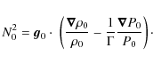
Seeking harmonic solutions in time, the variable are written
![$\displaystyle \left[- \omega^4 + \omega^2 c_{\rm s}^2 f \vec{\nabla} \cdot \left(\frac{{\vec g}_0}{c_{\rm s}^2 f}\right) \right]\hat{P}$](/articles/aa/full_html/2009/24/aa11165-08/img228.png) |
|||
![$\displaystyle \hspace*{4mm}
+ \left[\omega^2 \left(1 + \frac{c_{\rm s}^2 N_0^2}...
..._0^2 {\vec g}_0 }{g_0^2 f}\right) \right]
{\vec g}_0 \cdot \vec{\nabla} \hat{P}$](/articles/aa/full_html/2009/24/aa11165-08/img229.png) |
|||
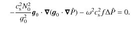 |
(A.4) |
We then look for a function ![]() such that the substitution
such that the substitution
![]() eliminates the first derivative term. The result is given by Eq. (10) where
eliminates the first derivative term. The result is given by Eq. (10) where
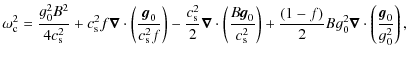
where
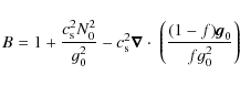

The

The expression of
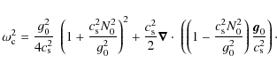
For polytropes
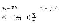
Equation (A.9) can then be simplified to give Eq. (12). We note that while the
A.2 Eikonal equation
We look for wave-like solutions (9) of the normal form of the perturbation Eq. (10) under the
assumption that ![]() the ratio between the wavelength of the solution and
the background typical lengthscale is very small.
Accordingly, the solution is expanded as
the ratio between the wavelength of the solution and
the background typical lengthscale is very small.
Accordingly, the solution is expanded as
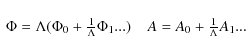
and the eikonal equation corresponds to the leading order of the expanded solution.
The highest
![]() terms verify
terms verify
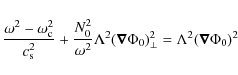
where the
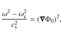 |
(A.13) |
which corresponds to the dispersion relation of acoustic waves. The
On the other hand, if
![]() ,
then we obtain
,
then we obtain
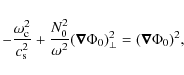 |
(A.14) |
which corresponds to gravity waves. This relation has been obtained under the assumption that the Coriolis force is negligible. While justified for high-frequency acoustic waves, this assumption is not necessarily true for gravity waves where the frequency is limited by
Finally, the next order of the expansion (A.11) yields the amplitude A0 in terms of ![]() (see for example Lighthill 1978).
(see for example Lighthill 1978).
Appendix B: Properties of the PSS
Two specific properties of the
![]() PSS are considered below. First,
we check in the non-rotating case that the distance d can be chosen so that all relevant trajectories intersect
the
PSS are considered below. First,
we check in the non-rotating case that the distance d can be chosen so that all relevant trajectories intersect
the
![]() curve. Second, we define a coordinate system of the PSS that ensures that
any surface of the PSS is conserved by the dynamics.
curve. Second, we define a coordinate system of the PSS that ensures that
any surface of the PSS is conserved by the dynamics.
B.1 Choice of the distance to the stellar surface
In the non-rotating case, Eq. (21) enables to characterise the trajectories that do not cross the PSS for a given value of d,
the distance to the stellar surface.
The radius of the internal caustic of
these trajectories ![]() must be such that
must be such that
![]() .
Using the definition of
.
Using the definition of ![]() and assuming that
and assuming that
![]() implies that
implies that
![]() .
According to
the relation between
.
According to
the relation between ![]() and
and ![]() ,
the degree of the corresponding mode
,
the degree of the corresponding mode
![]() (see Eq. (23) in
Sect. 4.1),
we find that these trajectories are associated with high-degree modes (
(see Eq. (23) in
Sect. 4.1),
we find that these trajectories are associated with high-degree modes (
![]() )
for the chosen value of
)
for the chosen value of
![]() and for
and for
![]() ,
where
,
where ![]() is the lowest acoustic mode frequency of the stellar model under consideration.
These modes are thus irrelevant for asteroseismology since their amplitude strongly
cancels out when integrated over the visible disk.
is the lowest acoustic mode frequency of the stellar model under consideration.
These modes are thus irrelevant for asteroseismology since their amplitude strongly
cancels out when integrated over the visible disk.
B.2 Area-preserving coordinates of the PSS
For a PSS defined by
![]() ,
we show here that
,
we show here that
![]() ,
the colatitude, and
,
the colatitude, and
![]() ,
,
![]() the angular component of
the angular component of ![]() in the natural basis associated with the coordinate system
in the natural basis associated with the coordinate system
![]() are area-preserving coordinates of the PSS.
are area-preserving coordinates of the PSS.
First we show that, for a general coordinate system xi, the spatial coordinates xi and
the covariant component
![]() of the vector
of the vector
![]() in the natural basis are conjugate variables of the Hamiltonian H given by Eq. (17).
The natural basis associated to a coordinate system xi is defined by
in the natural basis are conjugate variables of the Hamiltonian H given by Eq. (17).
The natural basis associated to a coordinate system xi is defined by
![]() where
where
![]() .
The contravariant component
.
The contravariant component
![]() of the velocity
of the velocity
![]() thus verifies
thus verifies
![]() .
(The notation
.
(The notation ![]() denotes a derivative with
respect to the time-like coordinate t).
If
denotes a derivative with
respect to the time-like coordinate t).
If
![]() is the Lagrangian of a system expressed in a coordinate system xi, it is well
known that a Legendre transformation leads to a Hamiltonian
is the Lagrangian of a system expressed in a coordinate system xi, it is well
known that a Legendre transformation leads to a Hamiltonian
![]() where
where
![]() is conjugate to xi.
The Lagrangian
is conjugate to xi.
The Lagrangian
![]() being associated with the Hamiltonian H given by Eq. (17),
the momentum variable pican be simply computed
being associated with the Hamiltonian H given by Eq. (17),
the momentum variable pican be simply computed
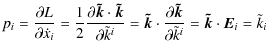 |
(B.1) |
thus showing that
Moreover, for a given conjugate coordinate system
[xi, pi], the coordinates
[x2,x3,p2,p3] of the PSS defined
by
![]() are known to be area-preserving (Ott 1993).
Thus, in our case,
are known to be area-preserving (Ott 1993).
Thus, in our case,
![]() is a conjugate coordinate system for the reduced Hamiltonian
is a conjugate coordinate system for the reduced Hamiltonian ![]() and the system
and the system
![]() is area-preserving for the PSS
is area-preserving for the PSS
![]() .
The natural basis and its conjugate reads
.
The natural basis and its conjugate reads
![]() and
and
![]() in terms of the unit vector associated with the spherical coordinates
in terms of the unit vector associated with the spherical coordinates
![]() .
Thus, with respect to the wavevector components in spherical coordinates
.
Thus, with respect to the wavevector components in spherical coordinates
![]() ,
the
,
the
![]() component reads
component reads
![]() .
.
Appendix C: Calculation of phase space volumes
Following the Monte-Carlo quadrature method (Press et al. 1992), ![]() points are randomly
chosen in a known volume
points are randomly
chosen in a known volume ![]() that includes the volume V to be computed.
The proportion of points
inside V approximates the ratio
that includes the volume V to be computed.
The proportion of points
inside V approximates the ratio
![]() ,
thus providing an estimated value of V.
The standard deviation error yields an estimate of the relative error,
,
thus providing an estimated value of V.
The standard deviation error yields an estimate of the relative error,
![]() ,
showing that the sampling volume
,
showing that the sampling volume ![]() has to be as close as possible to the volume Vand that the number of sampling points must be large.
has to be as close as possible to the volume Vand that the number of sampling points must be large.
In our case, the main practical issue is thus to determine if a given point in phase space is inside or outside
the 4-dimensional volume to be computed.
The two volumes that we computed are specified by two limiting frequencies
![]() and for each value of
and for each value of
![]() by the 3D volume inside a given 2D torus.
The first torus considered
separates the whispering gallery region from the chaotic region, its imprint on the
by the 3D volume inside a given 2D torus.
The first torus considered
separates the whispering gallery region from the chaotic region, its imprint on the
![]() PSS being shown in Fig. C.1.
The volume inside this torus includes the large chaotic region, as well as the island chains around the 2-period and 6-period orbits.
The second volume corresponds to the 2-period island chain and is delimited by a torus also shown in Fig. C.1.
PSS being shown in Fig. C.1.
The volume inside this torus includes the large chaotic region, as well as the island chains around the 2-period and 6-period orbits.
The second volume corresponds to the 2-period island chain and is delimited by a torus also shown in Fig. C.1.
To determine whether a given point
![]() is inside or outside these volumes,
one could construct the
is inside or outside these volumes,
one could construct the
![]() PSS associated to the value of the
Hamiltonian
PSS associated to the value of the
Hamiltonian
![]() ,
advance the dynamics from
,
advance the dynamics from
![]() until the trajectory cross the
until the trajectory cross the
![]() PSS,
and find out whether the crossing point is inside or outside the torus.
Here, to simplify the procedure, we used the fact that the
PSS,
and find out whether the crossing point is inside or outside the torus.
Here, to simplify the procedure, we used the fact that the
![]() PSS plotted against the scaled wavenumber
PSS plotted against the scaled wavenumber
![]() appeared to be insensitive to values of the frequency
appeared to be insensitive to values of the frequency ![]() in the domain considered. We thus consider the point
in the domain considered. We thus consider the point
![]() and determine its location in the scaled phase space
computed for a given frequency. To control this supposedly weak frequency effect the computation has been performed
for the two extreme frequencies
and determine its location in the scaled phase space
computed for a given frequency. To control this supposedly weak frequency effect the computation has been performed
for the two extreme frequencies
![]() and
and
![]() .
Moreover, instead of advancing the dynamics up to the
.
Moreover, instead of advancing the dynamics up to the
![]() PSS, we construct a local PSS (either from a
PSS, we construct a local PSS (either from a
![]() surface
or a
surface
or a
![]() surface)
to compare the location of the
surface)
to compare the location of the
![]() point with the local imprint of the delimiting torus.
In practice, the imprint of the delimiting torus is not a continuous curve as the torus is actually obtained
from a space filling trajectory on the torus. We therefore follow such a trajectory over a sufficiently
large number of time step to increase the number of point of the torus imprint on the different PSS.
This procedure has been tested using trajectories which are known to be either inside or outside the torus
(like for example trajectories on nested tori inside the 2-period island chain). The number of points wrongly
located by this procedure can be made small enough to have a negligible effect when compared to the statistical error on the volume determination.
Furthermore, the integration domain has been divided into three subdomains following the pseudo-radial direction
point with the local imprint of the delimiting torus.
In practice, the imprint of the delimiting torus is not a continuous curve as the torus is actually obtained
from a space filling trajectory on the torus. We therefore follow such a trajectory over a sufficiently
large number of time step to increase the number of point of the torus imprint on the different PSS.
This procedure has been tested using trajectories which are known to be either inside or outside the torus
(like for example trajectories on nested tori inside the 2-period island chain). The number of points wrongly
located by this procedure can be made small enough to have a negligible effect when compared to the statistical error on the volume determination.
Furthermore, the integration domain has been divided into three subdomains following the pseudo-radial direction ![]() .
This enables to limit the ratio
.
This enables to limit the ratio
![]() as the sampling volumes can be more easily reduced in each subdomain.
as the sampling volumes can be more easily reduced in each subdomain.
![\begin{figure}
\par\includegraphics[width=8.4cm,clip]{11165fig10.eps}
\end{figure}](/articles/aa/full_html/2009/24/aa11165-08/img298.png) |
Figure C.1:
(Colour online) Intersection of two trajectories with the PSS at
|
| Open with DEXTER | |
Accordingly, the number of modes within the 2-period island chain is ![]() if we use the bounding torus computed for
if we use the bounding torus computed for
![]() and
and ![]() for
for
![]() .
The effect of changing the frequency is small in this case and the number of modes
can be estimated to
.
The effect of changing the frequency is small in this case and the number of modes
can be estimated to ![]() .
Likewise, the number of modes outside the whispering gallery region is
.
Likewise, the number of modes outside the whispering gallery region is ![]() for
for
![]() bounding torus
and
bounding torus
and ![]() for
for
![]() .
The frequency effect is stronger but still reasonable for the present purpose. We took the mean value of 270 modes with an error of
.
The frequency effect is stronger but still reasonable for the present purpose. We took the mean value of 270 modes with an error of ![]() mode.
mode.
Appendix D: Calculation of the disk-integration factor
According to the definition of the disk-integration factor, Eq. (37), we are led to calculate integrals of the form
where
We used two methods to compute the integral I. The first one is approximate because it assumes that the visibility curve is contained in a plane, but it is easy to compute accurately. The second method does not make this assumption but requires more computing time to complete accurate calculations.
The vector
![]() at the star's surface reads as
at the star's surface reads as
 |
(D.3) |
where
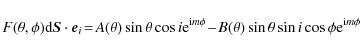
where
D.1 First method
The colatitude verifying
![]() for
for ![]() is denoted
is denoted
![]() .
As the inclination angle ican be restricted to
.
As the inclination angle ican be restricted to
![]() ,
we have
,
we have
![]() ,
and the angle
,
and the angle ![]() defined as
defined as
![]() verifies
verifies
![]() .
We assume that the visibility curve is the intersection of the stellar surface with the plane
.
We assume that the visibility curve is the intersection of the stellar surface with the plane
![]() ,
where the vector
,
where the vector
![]() of Cartesian coordinates
of Cartesian coordinates
![]() is normal to this plane.
Then, the integral is most simply calculated in the
coordinate system in which the polar axis is aligned with the direction of the vector
is normal to this plane.
Then, the integral is most simply calculated in the
coordinate system in which the polar axis is aligned with the direction of the vector
![]() .
This coordinate system results from a rotation of angle
.
This coordinate system results from a rotation of angle ![]() around the y axis of the
original coordinate system, the
new angular variables being denoted
around the y axis of the
original coordinate system, the
new angular variables being denoted ![]() and
and ![]() .
.
To express the integrand in these coordinates, we use the formula relating the spherical harmonics in both systems:
 |
(D.7) |
where
Integrating over the longitude
 |
(D.10) |
where we use the relations
 |
(D.11) |
| (D.12) |
and defined
To determine the coefficients
It follows that
 |
(D.16) |
so that the integral now reads
where


the
D.2 Second method
The visibility curve is no longer assumed to be planar. The integration over the visible surface is first performed in the azimuthal
direction and then in latitude. If
![]() ,
the integration is between 0 and
,
the integration is between 0 and ![]() ,
while in the interval
,
while in the interval
![]() one has to integrate between the two limiting azimuths
one has to integrate between the two limiting azimuths
![]() and
and
![]() verifying
verifying
![]() .
The integration domain is thus divided in two sub-domains, such that
.
The integration domain is thus divided in two sub-domains, such that
![\begin{displaymath}S_v = \left[0, \frac{\pi}{2}-\alpha \right] \times [0,2 \pi ]...
...a \right] \times \left[ -{\phi}_{\rm L},{\phi}_{\rm L}\right].
\end{displaymath}](/articles/aa/full_html/2009/24/aa11165-08/img360.png) |
(D.24) |
According to Eq. (D.4), the integration over
 |
(D.25) |
where
D.3 Tests
The methods have been tested in the case of an uniformly distributed function on the surface of an ellipsoïd where they should both give the same result. Then, the error introduced by the approximation of method 1 is estimated in the case of a Roche model surface.
D.3.1 Ellipsoïd
The surface being a quadric, the visibility curve is planar. Method 1 is therefore exact and should give the same result as method 2. In addition, the visible surface (obtained by taking F=1) can be obtained analytically. Indeed, the dimensionless equation of the ellipsoïd is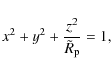 |
(D.26) |
and in spherical coordinates
where the distance have been normalized by the equatorial radius
By definition of the angle

In addition, using Eq. (D.28) and the relation between the Cartesian and spherical coordinates, the equation of the intersection between the plane
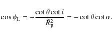
Thus,
| (D.31) |
is defined if
The visible surface can be calculated analytically as the visible curve is an ellipse.
This can be seen
using the Cartesian coordinates obtained by the rotation of angle ![]() about the Oyaxis:
about the Oyaxis:
The curve is then contained in the plane z'=0 and verifies
 |
(D.35) |
The surface of this ellipse can be calculated as well as its projection in the direction
Both methods were successfully tested against this analytical expression. Method 1 is simpler because it does not require a numerical integration. It is also very accurate, although it is necessary to use the analytical value of
D.3.2 Method 1 versus Method 2
Method 1 is approximate because it assumes that the curve on the surface verifying
using either the correct value of
In Fig. D.1, the relative error on the projected visible surface due to method 1 is plotted for Roche model surfaces of different flatness.
![\begin{figure}
\par\includegraphics[width=9cm,clip]{11165fig11.eps}
\end{figure}](/articles/aa/full_html/2009/24/aa11165-08/img392.png) |
Figure D.1: Relative error of the projected visible surface computed with method 1for Roche models of different flatnesses: 0.1526 (dot-dashed), 0.2594 (dotted) 0.2804 (dashed), 0.3092 (continuous line). |
| Open with DEXTER | |
It appears that, except for the near critical values of the flatness, the visible surface that is not considered by method 1 is a very small fraction of the total visible surface. Using method 1 is therefore a good approximation in these cases. For near critical flatness, the difference remains small, although it can be useful to test the results of method 1 with method 2.
References
- Anosov, D. V. 1967, Proc. Steklov. Inst. Math., 90, 1
- Ballot, J., Turck-Chièze, S., & García, R. A. 2004, A&A, 423, 1051 [NASA ADS] [CrossRef] [EDP Sciences]
- Benenti, G., Casati, G., Montangero, S., & Shepelyansky, D. L. 2002, Eur. Phys. J. D, 20, 293 [NASA ADS] [CrossRef] [EDP Sciences]
- Berry, M. V., & Tabor, M. 1977, Proc. R. Soc. A, 356, 375 [NASA ADS] [CrossRef] (In the text)
- Berry, M. V., & Robnik, M. 1984, J. Phys. A, 17, 2413 [NASA ADS] [CrossRef] (In the text)
- Bluemel, R., Antonsen, T. Jr., Georgeot, B., Ott, E., & Prange, R. E. 1996a, Phys. Rev. Lett., 76, 2476 [NASA ADS] [CrossRef]
- Bluemel, R., Antonsen, T. Jr., Georgeot, B., Ott, E., & Prange, R. E. 1996b, Phys. Rev. E, 53, 3284 [NASA ADS] [CrossRef]
- Bohigas, O., Giannoni, M.-J., & Schmit, C. 1984, Phys. Rev. Lett., 52, 1 [NASA ADS] [CrossRef]
- Bohigas, O., Tomsovic, S., & Ullmo, D. 1993, Phys. Rep., 223, 43 [NASA ADS] [CrossRef] (In the text)
- Born, M., & Wolf, E. 1999, Principles of optics, 7th edn. (Cambridge Univ. Press) (In the text)
- Bornatici, M., & Maj, O. 2003, Plasma Phys. Control. Fusion, 45, 707 [NASA ADS] [CrossRef]
- Brown, M. G., Colosi, J. A., Tomsovic, S., et al. 2003, J. Acoust. Soc. Am., 113, 2533 [NASA ADS] [CrossRef] (In the text)
- Chang, S.-J., & Shi, K.-J. 1986, Phys. Rev. A, 34, 7 [NASA ADS] [CrossRef] (In the text)
- Chirikov, B. V. 1979, Phys. Rep., 52, 263 [NASA ADS] [CrossRef]
- Christensen-Dalsgaard, J. 1980, MNRAS, 190, 765 [NASA ADS] (In the text)
- Christensen-Dalsgaard, J., & Thompson, M. J. 1999, A&A, 350, 852 [NASA ADS] (In the text)
- Deubner, F.-L., & Gough, D. 1984, ARA&A, 22, 593 [NASA ADS] [CrossRef]
- Einstein, A. 1917, Deutsche Phys. Ges., 19, 82 (In the text)
- Ellegaard, C., Guhr, T., Lindemann, K., Nygaard, J., & Oxborrow, M. 1996, Phys. Rev. Lett., 77, 4918 [NASA ADS] [CrossRef] (In the text)
- Espinosa Lara, F., & Rieutord, M. 2007, A&A, 470, 1013 [NASA ADS] [CrossRef] [EDP Sciences]
- Giannoni, M.-J., Voros, A., & Zinn-Justin, J. (ed.) 1991, Les Houches Lectures Session LII (North-Holland)
- Gough, D. O. 1990, in Progress of Seismology of the Sun and Stars, ed. Y. Osaki, & H. Shibahashi, Lecture Notes in Physics (Springer-Verlag), 367, 283
- Gough, D. O. 1993, in Les Houches Lectures Session XLVIII, ed. J.-P. Zahn, & J. Zinn-Justin (North-Holland), 399 (In the text)
- Gutzwiller, M. 1990, Chaos in Classical and Quantum Mechanics (Springer)
- Hansen, C. J., & Kawaler, S.D. 1994, Stellar interiors (Springer) (In the text)
- Heller, E. J. 1984, Phys. Rev. Lett., 53, 1515 [NASA ADS] [CrossRef] (In the text)
- Keller, J. B., & Rubinow, S. I. 1960, Ann. Phys., 9, 24 [NASA ADS] [CrossRef] (In the text)
- Kogelnik, H., & Li, T. 1966, Appl. Opt., 5, 1550 [NASA ADS] [CrossRef] (In the text)
- Kosovichev, A. G., & Perdang, J. 1988, in Seismology of the Sun and Sun-Like Stars, ESA SP-286, 539 (In the text)
- Lazutkin, V. F. 1993, KAM Theory and Semiclassical Approximations to Eigenfunctions (Springer)
- Lichtenberg, A., & Lieberman, M. 1992, Regular and Chaotic Dynamics (Springer)
- Lighthill, J. 1978, Waves in Fluids (Cambridge University Press) (In the text)
- Lignières, F., & Georgeot, B. 2008, Phys. Rev. E, 78, 016215 [NASA ADS] [CrossRef] (In the text)
- Lignières, F., Rieutord, M., & Reese, D. 2006, A&A, 455, 607 [NASA ADS] [CrossRef] [EDP Sciences]
- Lovekin, C. C., & Deupree, R. G. 2008, ApJ, 679, 1499 [NASA ADS] [CrossRef]
- MacGregor, K. B., Jackson, S., Skumanich, A., & Metcalfe, T. S. 2007, ApJ, 663, 560 [NASA ADS] [CrossRef]
- Nöckel, J. U., & Stone, A. D. 1997, Nature, 385, 45 [NASA ADS] [CrossRef] (In the text)
- Ott, E. 1993, Chaos in Dynamical Systems (Cambridge Univ. Press)
- Pekeris, C. L. 1938, ApJ, 88, 189 [NASA ADS] [CrossRef] (In the text)
- Percival, I. C. 1973, J. Phys. B, 6, L229 [NASA ADS] [CrossRef] (In the text)
- Perdang, J. 1988, in Multimode Stellar Pulsations, ed. G. Kovacs, L. Szabados, & B. Szeidl (Budapest: Kultura), 209 (In the text)
- Permitin, G. V., & Smirnov, A. I. 1996, JETP, 82, 395 [NASA ADS]
- Prange, R. E., Ott, E., Antonsen, T. Jr, Georgeot, B., & Bluemel, R. 1996, Phys. Rev. E, 53, 207 [NASA ADS] [CrossRef] (In the text)
- Press, W. H., Teukolsky, S. A., Vetterling, W. T., & Flannery, B. P. 1992, Numerical Recipes, 2th edn. (Cambridge Univ. Press) (In the text)
- Rieutord, M., Dintrans, B., Lignières, F., Corbard, T., & Pichon, B. 2005, in Semaine de l'Astrophysique Française, ed. F. Combes et al., Conf. Ser., 759 (EDP Sciences) (In the text)
- Reese, D. 2007, Ph.D. Thesis
- Reese, D., Lignières, F., & Rieutord, M. 2006, A&A, 455, 621 [NASA ADS] [CrossRef] [EDP Sciences]
- Reese, D., Lignières, F., & Rieutord, M. 2008, A&A, 481, 449 [NASA ADS] [CrossRef] [EDP Sciences] (In the text)
- Reese, D. R., MacGregor, K. B., Jackson, S., Skumanich, A., & Metcalfe, T. S. 2009, A&A, in press [arXiv:0903.4854] (In the text)
- Roxburgh, I. W. 2006, A&A, 454, 883 [NASA ADS] [CrossRef] [EDP Sciences]
- Roxburgh, I. W., & Vorontsov, S. V. 2000, MNRAS, 317, 141 [NASA ADS] [CrossRef]
- Sauer, T., Grebogi, C., & Yorke, J. A. 1997, Phys. Rev. Lett., 79, 59 [NASA ADS] [CrossRef]
- Schack, R., & Caves, C. M. 1993, Phys. Rev. Lett., 71, 525 [NASA ADS] [CrossRef]
- Stöckmann, H.-J., & Stein, J. 1990, Phys. Rev. Lett., 64, 2215 [NASA ADS] [CrossRef] (In the text)
- Tassoul, M. 1980, ApJS, 43, 469 [NASA ADS] [CrossRef]
- Tassoul, M. 1990, ApJ, 358, 313 [NASA ADS] [CrossRef]
- Vandakurov, Y. V. 1967, AZh, 44, 786 [NASA ADS]
- Vorontsov, S. V. 1988, in Advances in Helio- and Asteroseismology, ed. J. Christensen-Dalsgaard, & S. Frandsen (Reidel), IAU Symp., 123, 151
- Weyl, H. 1912, Math. Ann., 71, 441 [CrossRef] (In the text)
- Wigner, E. P. 1932, Phys. Rev., 40, 749 [NASA ADS] [CrossRef] (In the text)
All Figures
| |
Figure 1:
(Colour online) Intersection of an outgoing acoustic ray (red/arrow headed) with the
|
| Open with DEXTER | |
| In the text | |
| |
Figure 2:
(Colour online) PSS at
|
| Open with DEXTER | |
| In the text | |
| |
Figure 3:
Three
|
| Open with DEXTER | |
| In the text | |
| |
Figure 4:
Three
|
| Open with DEXTER | |
| In the text | |
| |
Figure 5:
Three
|
| Open with DEXTER | |
| In the text | |
| |
Figure 6:
(Colour online) Four axisymmetric modes and their phase space representation: a) a 2-period island mode (blue/dark grey),
b) a chaotic mode (red/grey), c) a 6-period island mode (magenta/light grey), and d) a whispering gallery
mode (green/light grey). The amplitude distribution of the
scaled mode |
| Open with DEXTER | |
| In the text | |
| |
Figure 7: Frequency subspectra of four classes of axisymmetric modes: a) the 2-period island modes, b) the chaotic modes antisymmetric with respect to the equator, c) the 6-period island modes, and d) some whispering gallery modes. For the subspectra a) and d), the height of the vertical bar specifies one of the two quantum numbers characterising the mode. |
| Open with DEXTER | |
| In the text | |
| |
Figure 8:
Integrated spacing distribution |
| Open with DEXTER | |
| In the text | |
| |
Figure 9:
(Colour online) Frequency spectra of axisymmetric modes where the amplitude is given by the normalized disk-averaging factor D(i) for
a star seen pole-on i =0 and equator-on |
| Open with DEXTER | |
| In the text | |
| |
Figure C.1:
(Colour online) Intersection of two trajectories with the PSS at
|
| Open with DEXTER | |
| In the text | |
| |
Figure D.1: Relative error of the projected visible surface computed with method 1for Roche models of different flatnesses: 0.1526 (dot-dashed), 0.2594 (dotted) 0.2804 (dashed), 0.3092 (continuous line). |
| Open with DEXTER | |
| In the text | |
Copyright ESO 2009
Current usage metrics show cumulative count of Article Views (full-text article views including HTML views, PDF and ePub downloads, according to the available data) and Abstracts Views on Vision4Press platform.
Data correspond to usage on the plateform after 2015. The current usage metrics is available 48-96 hours after online publication and is updated daily on week days.
Initial download of the metrics may take a while.