| Issue |
A&A
Volume 500, Number 2, June III 2009
|
|
|---|---|---|
| Page(s) | 763 - 768 | |
| Section | Extragalactic astronomy | |
| DOI | https://doi.org/10.1051/0004-6361/200811351 | |
| Published online | 29 April 2009 | |
Determination of the cosmic far-infrared background level with the ISOPHOT instrument![[*]](/icons/foot_motif.png) , (Research Note)
, (Research Note)
M. Juvela1 - K. Mattila1 - D. Lemke2 - U. Klaas2 - C. Leinert2 - Cs. Kiss3
1 - Observatory, University of Helsinki, PO Box 14, 00014 Helsinki, Finland
2 -
Max-Planck-Institut für Astronomie, Königstuhl 17, 69117 Heidelberg, Germany
3 -
Konkoly Observatory of the Hungarian Academy of Sciences, PO Box 67, 1525 Budapest, Hungary
Received 15 November 2008 / Accepted 8 April 2008
Abstract
Context. The cosmic infrared background (CIRB) consists mainly of the integrated light of distant galaxies. In the far-infrared the current estimates of its surface brightness are based on the measurements of the COBE satellite. Independent confirmation of these results is still needed from other instruments.
Aims. In this paper we derive estimates of the far-infrared CIRB using measurements made with the ISOPHOT instrument aboard the ISO satellite. The results are used to seek further confirmation of the CIRB levels that have been derived by various groups using the COBE data.
Methods. We study three regions of very low cirrus emission. The surface brightness observed with the ISOPHOT instrument at 90, 150, and 180 ![]() m is correlated with hydrogen 21 cm line data from the Effelsberg radio telescope. Extrapolation to zero hydrogen column density gives an estimate for the sum of extragalactic signal plus zodiacal light. The zodiacal light is subtracted using ISOPHOT data at shorter wavelengths. Thus, the resulting estimate of the far-infrared CIRB is based on ISO measurements alone.
m is correlated with hydrogen 21 cm line data from the Effelsberg radio telescope. Extrapolation to zero hydrogen column density gives an estimate for the sum of extragalactic signal plus zodiacal light. The zodiacal light is subtracted using ISOPHOT data at shorter wavelengths. Thus, the resulting estimate of the far-infrared CIRB is based on ISO measurements alone.
Results. In the range 150 to 180 ![]() m, we obtain a CIRB value of 1.08
m, we obtain a CIRB value of 1.08 ![]() 0.32
0.32 ![]() 0.30 MJy sr-1 quoting statistical and systematic errors separately. In the 90
0.30 MJy sr-1 quoting statistical and systematic errors separately. In the 90 ![]() m band, we obtain a 2-
m band, we obtain a 2-![]() upper limit of 2.3 MJy sr-1.
upper limit of 2.3 MJy sr-1.
Conclusions. The estimates derived from ISOPHOT far-infrared maps are consistent with the earlier COBE results.
Key words: galaxies: evolution - cosmology: observations - infrared: galaxies
1 Introduction
The extragalactic background light (EBL) consists of the integrated light of all galaxies along the line of sight with possible additional contributions from intergalactic gas and dust and hypothetical decaying relic particles. It plays an important role in cosmological studies because most of the gravitational and fusion energy released in the universe since the recombination epoch is expected to reside in the EBL. Measurements of the cosmic infrared background, CIRB, help to address some central, but still largely open astrophysical problems, including the early evolution of galaxies, and the entire star formation history of the universe. An important issue is the balance between the UV-optical-NIR and the far-infrared backgrounds; the fraction of optical radiation lost by dust obscuration re-appears as dust emission at longer wavelengths. The absolute level of the CIRB, the fluctuations in the CIRB surface brightness, and the resolved bright end of the distribution of galaxies contributing to the CIRB all provide strong constraints on the models of galaxy evolution through different epochs. For reviews, see Hauser & Dwek (2001) and Lagache et al. (2005). The full analysis of the data from the DIRBE (Hauser et al. 1998; Schlegel et al. 1998) and FIRAS (Fixen et al. 1997) experiments indicated a CIRB at a surprisingly high level of ![]() 1 MJy sr-1 between 140 and 240
1 MJy sr-1 between 140 and 240 ![]() m. Preliminary results had been obtained by Puget et al. (1996). Lagache et al. (1999) claimed the detection of a component of Galactic dust emission associated with
warm ionised medium. The removal of this component led to a CIRB level of 0.7 MJy sr-1 at 140
m. Preliminary results had been obtained by Puget et al. (1996). Lagache et al. (1999) claimed the detection of a component of Galactic dust emission associated with
warm ionised medium. The removal of this component led to a CIRB level of 0.7 MJy sr-1 at 140 ![]() m.
m.
Because the FIR CIRB is important for cosmology these results need to be confirmed by independent measurements. The ISOPHOT instrument (Lemke et al. 1996), flown on the cryogenic, actively cooled ISO satellite, provided the capabilities for this. The ISOPHOT observation technique was different from COBE: (1) with its relatively small f.o.v. ISOPHOT was capable of looking into the darkest spots between the cirrus clouds; (2) ISOPHOT had high sensitivity in the important FIR window at 120-200 ![]() m; (3) with its good spatial and multi-wavelength FIR spectral sampling ISOPHOT gave an improved possibility of separating and eliminating the emission of Galactic
cirrus. The primary goal of the ISOPHOT EBL project is the determination of the absolute level of the FIR CIRB. The other goals are the measurement of the spatial CIRB fluctuations and the detection of the bright end of the FIR point source distribution. The bright end of the galaxy population contributing to the FIR CIRB signal was analysed by Juvela et al. (2000).
m; (3) with its good spatial and multi-wavelength FIR spectral sampling ISOPHOT gave an improved possibility of separating and eliminating the emission of Galactic
cirrus. The primary goal of the ISOPHOT EBL project is the determination of the absolute level of the FIR CIRB. The other goals are the measurement of the spatial CIRB fluctuations and the detection of the bright end of the FIR point source distribution. The bright end of the galaxy population contributing to the FIR CIRB signal was analysed by Juvela et al. (2000).
2 The method
We examine three regions of low cirrus emission that were mapped with the ISOPHOT at 90, 150, and 180 ![]() m. Because of the high sensitivity of the ISOPHOT FIR detectors, we can directly correlate HI with ISOPHOT measurements for each FIR band separately. In the case of DIRBE, the original analysis performed by the DIRBE team used 100
m. Because of the high sensitivity of the ISOPHOT FIR detectors, we can directly correlate HI with ISOPHOT measurements for each FIR band separately. In the case of DIRBE, the original analysis performed by the DIRBE team used 100 ![]() m as an ISM template and, therefore, the accuracy of the CIRB detections at 140
m as an ISM template and, therefore, the accuracy of the CIRB detections at 140 ![]() m and 240
m and 240 ![]() m also depended on the systematic uncertainties of the 100
m also depended on the systematic uncertainties of the 100 ![]() m data (Hauser et al. 1998; Arendt et al. 1998).
m data (Hauser et al. 1998; Arendt et al. 1998).
The HI lines are optically thin and their intensity traces the amount of neutral hydrogen along the line-of-sight. The level of FIR emission associated with the ionised medium is still uncertain and we will consider the possible effects later in the analysis.
As a first step, a relation between the HI line area and the FIR surface brightness is obtained. The relation depends on the gas-to-dust ratio, grain properties, and the radiation field illuminating the interstellar medium (ISM) along the line-of-sight. No significant variations have been observed in the gas-to-dust ratio apart from those associated with large scale metallicity variations. Similarly, because of the diffuse nature of the HI clouds, no small scale changes in the intrinsic dust properties or dust temperature are expected. Under these conditions the FIR signal should have a linear dependence on the HI column density. Because each field is considered individually, possible differences in the HI-FIR relation towards different regions can and will be taken into account. For each field, an extrapolation to zero HI intensity eliminates emission associated with the neutral ISM (for details, see Sect. 4.1). The remaining signal is equal to the sum of the zodiacal light (ZL) and the CIRB. These components are not removed because they are uncorrelated with the HI emission. Furthermore, the ZL has a smooth distribution and remains practically constant within each of the areas covered by individual ISOPHOT maps (see Ábrahám et al. 1997). If the ZL level is known, the absolute value of the CIRB can be obtained. The ZL estimation is described in detail in Sect. 4.2.
3 Observations
We study three low surface brightness fields that are labelled NGP, EBL22, and EBL26. The field NGP is located at the North Galactic Pole, the field EBL22 is similarly at a high ecliptic latitude, while the third one, EBL26, lies close to the ecliptic plane (see Table B.3). EBL26 was selected as a field with high ZL level with the purpose of estimating the ZL contribution at the different wavelengths observed in this project.
The observations of the hydrogen 21 cm line were made with the Effelsberg radio telescope in May 2002. The telescope beam has a FWHM of 9 arcmin. The areas mapped with the ISOPHOT instrument were covered with pointings at steps of FWHM/2. The stray radiation was removed with a program developed by Kalberla (see Kalberla 1982; Hartmann et al. 1996; Kalberla et al. 2005).
For details of the observations of the EBL fields and the associated data reduction, see Appendix B. The principles of ISOPHOT data reduction and calibration of surface brightness measurements are explained in Appendix A.
4 Analysis and results
4.1 Subtraction of Galactic cirrus emission using HI data
The FIR surface brightness was correlated at each observed wavelength with the integrated line area of the HI spectra. At each observed HI position the average FIR signal was calculated using spatial weighting with a Gaussian with FWHM equal to 9
![]() .
Only those pointings are used where the centre of the Effelsberg beam falls inside the FIR map. In addition to the observational uncertainties, each data point was weighted in direct proportion to the fraction of the HI FWHM beam that was covered by FIR observations. Therefore, the data close to FIR map boundaries get lower weight in the following analysis.
.
Only those pointings are used where the centre of the Effelsberg beam falls inside the FIR map. In addition to the observational uncertainties, each data point was weighted in direct proportion to the fraction of the HI FWHM beam that was covered by FIR observations. Therefore, the data close to FIR map boundaries get lower weight in the following analysis.
The obtained correlations are shown in Fig. 1. For FIR observations the plotted error bars are based on the statistical uncertainties reported by the PIA.
The figures include linear fits that take into account the estimated uncertainties in both FIR and HI data. The slopes and zero points of the fit are given in Table 1. In field EBL26 there is a clear break in the relation above W(HI) = 200 K km s-1 that may indicate the
presence of molecular gas. There is also one fairly bright galaxy that is located in the region of higher cirrus emission and may have affected the correlation. Therefore, in the field EBL26 the linear fitting was carried out using only data below
![]() K km s-1. In the other fields the hydrogen column densities are in general smaller,
K km s-1. In the other fields the hydrogen column densities are in general smaller,
![]() K km s-1, so that the fraction of molecular gas can be expected to be insignificant.
K km s-1, so that the fraction of molecular gas can be expected to be insignificant.
The offsets thus obtained correspond to an extrapolation to zero HI column density. To the extent to which the remaining contributions of ionised and molecular gas can be ignored (see below), the values correspond to the sum of CIRB and the zodiacal light.
![\begin{figure}
\par\includegraphics[height=8.3cm,width=6cm,clip]{1351fg01.eps}\i...
...02.eps}\includegraphics[height=8.3cm,width=6cm,clip]{1351fg03.eps}
\end{figure}](/articles/aa/full_html/2009/23/aa11351-08/img15.png) |
Figure 1:
FIR surface brightness as a function of HI line area W(HI) in the three EBL fields, EBL22 ( left), EBL26 ( middle), and NGP ( right). Each point
corresponds to one pointing of the HI observations. The uncertainties in the HI line area are estimated based on the noise in velocity channels outside detected HI emission. For each HI spectrum the corresponding average FIR signal has been calculated using for weighting a Gaussian with FWHM = 9
|
| Open with DEXTER | |
4.2 Subtraction of the zodiacal light
The zodiacal light (ZL) emission is assumed to have a pure black body spectrum. The colour temperature of the spectrum depends on the ecliptic coordinates of the source and the solar elongation at the time of the observations. Leinert et al. (2002) have studied the variations of mid-infrared ZL spectra over the sky using a set of observations made with the ISOPHOT spectrometer. We use their results to fix the colour temperature of the ZL spectra.
The absolute intensity of the ZL emission in the FIR is estimated with the help of shorter wavelength ISOPHOT observations made using the ISOPHOT P detector in the absolute photometry observing mode PHT-05 (Laureijs et al. 2003). Because the observations were made in regions of low cirrus emission, the mid-infrared signal is completely dominated by the ZL. The measurements were carried out close to the larger raster maps, in terms of both time and position. Therefore, they give a good estimate for the zodiacal light emission present in the raster maps. FIR absolute photometry measurements were made at the same time and at the same positions. These are used to make a correction for the contribution that the interstellar dust has, conversely, on the measured mid-infrared values. The complete list of observations is given in Table B.2.
Table 1: Parameters of linear fits of FIR surface brightness versus the HI line area.
The derived ZL values obtained from the fits (ZL+cirrus) are listed in Table 2. The values are given at the nominal wavelengths assuming a spectrum
![]() const. The uncertainties were estimated based on the quality of the fits (see Appendix D). In fields EBL26 and NGP, because error estimate of each of the two measurements is itself uncertain, we conservatively take the average of the two error
estimates as the uncertainty of the mean.
const. The uncertainties were estimated based on the quality of the fits (see Appendix D). In fields EBL26 and NGP, because error estimate of each of the two measurements is itself uncertain, we conservatively take the average of the two error
estimates as the uncertainty of the mean.
Table 2: The estimated zodiacal light emission.
4.3 Estimated CIRB levels and their uncertainties
Table 3 lists the CIRB levels that are estimated based on the linear fits between FIR and HI data (Table 1) and the zodiacal light values of Table 2. The uncertainties are obtained by adding in quadrature the estimated errors of the offsets from Table 1, the errors of the zodiacal light values from
Table 2, and the error resulting from the dark current subtraction (see Appendix C),
 |
(1) |
The uncertainty due to the dark current is estimated to be
The results obtained for the three individual fields can be combined, deriving our final estimates for the CIRB and its uncertainty. In the case of the field EBL26 the values are relatively unprecise because of the high ZL level. This uncertainty is reflected in the error estimates. Combining the results we get average values -0.54 ![]() 0.65 MJy sr-1, 0.83
0.65 MJy sr-1, 0.83 ![]() 0.41 MJy sr-1,
1.26
0.41 MJy sr-1,
1.26 ![]() 0.37 MJy sr-1, at 90
0.37 MJy sr-1, at 90 ![]() m, 150
m, 150 ![]() m, and 180
m, and 180 ![]() m, respectively, as given in the last line of Table 3.
m, respectively, as given in the last line of Table 3.
The 90 ![]() m values are very low, because in both the EBL22 and EBL26 fields negative values are obtained. In the case of EBL26 the negative value is not surprising, because the expected CIRB level is only a small fraction of the zodiacal light which itself has a considerable statistical uncertainty. Therefore, the result is sensitive also to any systematic errors of the ZL
estimates. Apart from the results at 90
m values are very low, because in both the EBL22 and EBL26 fields negative values are obtained. In the case of EBL26 the negative value is not surprising, because the expected CIRB level is only a small fraction of the zodiacal light which itself has a considerable statistical uncertainty. Therefore, the result is sensitive also to any systematic errors of the ZL
estimates. Apart from the results at 90 ![]() m, the variation between fields is only slightly larger than expected on the basis of the quoted error estimates. At 150
m, the variation between fields is only slightly larger than expected on the basis of the quoted error estimates. At 150 ![]() m a negative value is obtained for EBL26 which, nevertheless, is less than 2-
m a negative value is obtained for EBL26 which, nevertheless, is less than 2-![]() below the highest values.
below the highest values.
At 90 ![]() m we can derive for EBL only an upper limit. The 150
m we can derive for EBL only an upper limit. The 150 ![]() m and 180
m and 180 ![]() m bands are close to each other and the CIRB values should be very similar. Therefore, based on the three fields and the two frequency bands, we can calculate, as a weighted average, an estimate for the CIRB in the range 150-180
m bands are close to each other and the CIRB values should be very similar. Therefore, based on the three fields and the two frequency bands, we can calculate, as a weighted average, an estimate for the CIRB in the range 150-180 ![]() m. The result is 1.08
m. The result is 1.08 ![]() 0.32 MJy sr-1. The result would not change significantly (less than 1-
0.32 MJy sr-1. The result would not change significantly (less than 1-![]() )
even if either EBL22 or EBL26 were omitted from the
analysis.
)
even if either EBL22 or EBL26 were omitted from the
analysis.
Table 3: Estimated level of the CIRB for the individual fields.
4.4 The reliability of the CIRB values
In addition to the statistical uncertainties, the results are affected by systematic errors. The CIRB estimates are not affected by the HI antenna temperature scale. However, the presence of unsubtracted stray radiation could affect the HI zero point of the HI data and, thus, lower the CIRB values. We cannot directly estimate the presence of residual stray radiation in the HI data. However, in Sect. B.3 we compare some of our HI spectra with data from the Leiden/Dwingeloo survey (Hartmann & Burton 1997; Kalberla et al. 2005) and we find that the residual stray radiation is likely to be less than
4 K km s-1 which, assuming a slope of 29 ![]() 10-3 MJy sr-1 (K km s-1)-1 (see Table 1), corresponds to 0.12 MJy sr-1. In this case HI stray radiation would not be a major source of error.
10-3 MJy sr-1 (K km s-1)-1 (see Table 1), corresponds to 0.12 MJy sr-1. In this case HI stray radiation would not be a major source of error.
The relative calibration of the ISOPHOT FIR cameras and the P-detectors directly affects the estimated FIR ZL levels and is probably the most important source of systematic errors. According to the ISOPHOT Handbook (Laureijs et al. 2003) the absolute accuracy of the C100 and C200 cameras and the P-detectors is typically of the order of 20%. If there were a difference of 10% in the relative calibration of the MIR and FIR bands, this would cause a similar percentual error to the ZL estimates. The fact that we obtained negative CIRB values at 90 ![]() m, especially when the absolute level of the ZL is high, suggests that the FIR ZL levels may have
been overestimated. The effect of an error of 10% would range from
m, especially when the absolute level of the ZL is high, suggests that the FIR ZL levels may have
been overestimated. The effect of an error of 10% would range from ![]() 2 MJy sr-1 at 90
2 MJy sr-1 at 90 ![]() m in the field EBL26 to
m in the field EBL26 to ![]() 0.2 MJy sr-1 at 150-180
0.2 MJy sr-1 at 150-180 ![]() m in the field NGP. Taking into account the relative weighting of the three fields, a 10% error in ZL corresponds to an uncertainty of 0.3 MJy sr-1 in the 150-180
m in the field NGP. Taking into account the relative weighting of the three fields, a 10% error in ZL corresponds to an uncertainty of 0.3 MJy sr-1 in the 150-180 ![]() m CIRB estimate. Assuming a systematic uncertainty of this magnitude, the CIRB estimate can be written as 1.08
m CIRB estimate. Assuming a systematic uncertainty of this magnitude, the CIRB estimate can be written as 1.08 ![]() 0.32
0.32 ![]() 0.30 MJy sr-1 where the first error estimate refers to statistical and the second to systematic
uncertainties.
0.30 MJy sr-1 where the first error estimate refers to statistical and the second to systematic
uncertainties.
At 90 ![]() m the negative value obtained for EBL26 carries very little weight and an additional 10% systematic uncertainty in the ZL would correspond to an additional uncertainty of 2 MJy sr-1. In EBL22 the CIRB values was -2.16
m the negative value obtained for EBL26 carries very little weight and an additional 10% systematic uncertainty in the ZL would correspond to an additional uncertainty of 2 MJy sr-1. In EBL22 the CIRB values was -2.16 ![]() 1.04 and a 10% systematic error in the ZL values would correspond to 0.77 MJy sr-1. The CIRB value is
1.04 and a 10% systematic error in the ZL values would correspond to 0.77 MJy sr-1. The CIRB value is ![]() 2-
2-![]() below zero and suggests that the ZL values may contain a systematic error of
below zero and suggests that the ZL values may contain a systematic error of ![]() 10-20% that has reduced the obtained CIRB values. In the field NGP the 90
10-20% that has reduced the obtained CIRB values. In the field NGP the 90 ![]() m CIRB estimate was 0.35
m CIRB estimate was 0.35 ![]() 0.74 MJy sr-1. Assuming a 10% systematic uncertainty in the ZL and adding the error estimates in quadrature, the CIRB estimate becomes 0.35
0.74 MJy sr-1. Assuming a 10% systematic uncertainty in the ZL and adding the error estimates in quadrature, the CIRB estimate becomes 0.35 ![]() 0.95 MJy sr-1 and we obtain a 2-
0.95 MJy sr-1 and we obtain a 2-![]() upper limit of 2.3 MJy sr-1.
upper limit of 2.3 MJy sr-1.
5 Discussion
5.1 Dust emission associated with ionised gas
Our analysis was based on the correlation of HI emission and FIR intensity. So far we have omitted the possible effect that dust mixed with ionised gas might have. The ionised component can affect the results only as far as it is uncorrelated with the HI emission.
Lagache et al. (2000) decomposed the DIRBE FIR intensity into components correlated with the neutral and the ionised medium. The column density of ionised hydrogen,
![]() ,
was estimated based on the H
,
was estimated based on the H![]() line. They found that the infrared emissivity of dust associated with the ionised medium would be very similar to the emissivity of dust within the neutral medium. However, Odegard et al. (2007) recently re-examined this issue, obtaining significantly lower emissivity values for the ionised medium. The derived 2-
line. They found that the infrared emissivity of dust associated with the ionised medium would be very similar to the emissivity of dust within the neutral medium. However, Odegard et al. (2007) recently re-examined this issue, obtaining significantly lower emissivity values for the ionised medium. The derived 2-![]() upper limit for the 100
upper limit for the 100 ![]() m emissivity per hydrogen ion was typically only 40% of the emissivity in the neutral atomic medium.
m emissivity per hydrogen ion was typically only 40% of the emissivity in the neutral atomic medium.
We use the all-sky H![]() map produced by Finkbeiner (2003) to examine the possible contribution of the ionised medium to the FIR emission. The resolution of the H
map produced by Finkbeiner (2003) to examine the possible contribution of the ionised medium to the FIR emission. The resolution of the H![]() data is 6
data is 6
![]() for fields EBL22 and EBL26 and one degree at the location of the field NGP. The average H
for fields EBL22 and EBL26 and one degree at the location of the field NGP. The average H![]() emission in the EBL22, EBL26, and NGP fields is
emission in the EBL22, EBL26, and NGP fields is ![]() 0.7 R,
0.7 R, ![]() 0.5 R, and
0.5 R, and ![]() 0.6 R, respectively. The H
0.6 R, respectively. The H![]() background contains small scale structure that may be caused by faint point sources, mainly stars. Therefore, the quoted H
background contains small scale structure that may be caused by faint point sources, mainly stars. Therefore, the quoted H![]() levels are not caused by the diffuse ISM only. For example, in NGP the H
levels are not caused by the diffuse ISM only. For example, in NGP the H![]() image is dominated by an unresolved (
image is dominated by an unresolved (![]() one degree) emission peak at the centre of the field, the nature of which remains unknown. Apart from this, the H
one degree) emission peak at the centre of the field, the nature of which remains unknown. Apart from this, the H![]() background does not show any significant gradients or correlation with the FIR emission. Therefore, we consider only the effect on the average FIR signal. Using the Lagache et al. (2000) conversion factors an H
background does not show any significant gradients or correlation with the FIR emission. Therefore, we consider only the effect on the average FIR signal. Using the Lagache et al. (2000) conversion factors an H![]() signal of 0.6 R would correspond to
signal of 0.6 R would correspond to ![]() 0.5 MJy sr-1 in the FIR. Therefore, the CIRB values could be overestimated by a similar amount. However, adopting the
Odegard et al. (2007) 1-
0.5 MJy sr-1 in the FIR. Therefore, the CIRB values could be overestimated by a similar amount. However, adopting the
Odegard et al. (2007) 1-![]() upper limits, the contribution from the ionised medium should remain below 0.1 MJy/sr. Furthermore, in our analysis we have correlated the FIR emission only with HI while in the quoted studies the FIR signal was correlated simultaneously with both HI and H+. Therefore, since HI and H+ are themselves correlated, the correction to be applied to our results should be correspondingly smaller. Therefore, we believe that the possible effects due to the presence of an ionised medium are small compared with the other
uncertainties given above.
upper limits, the contribution from the ionised medium should remain below 0.1 MJy/sr. Furthermore, in our analysis we have correlated the FIR emission only with HI while in the quoted studies the FIR signal was correlated simultaneously with both HI and H+. Therefore, since HI and H+ are themselves correlated, the correction to be applied to our results should be correspondingly smaller. Therefore, we believe that the possible effects due to the presence of an ionised medium are small compared with the other
uncertainties given above.
5.2 Dust emission associated with molecular gas
If molecular gas is present, the HI lines will underestimate the total column density of gas and, because the fraction of molecular gas increases with column density, the relation between FIR emission and the HI intensity becomes steeper. Our fields have low column density and, therefore, the fraction of molecular gas should be low. Hydrogen molecules cannot survive in clouds with visual extinction below
![]() and, consequently, no molecular gas should exist in clouds with column densities below
and, consequently, no molecular gas should exist in clouds with column densities below
![]()
![]() 1020 cm-2. Arendt et al. (1998) detected a steepening in the FIR vs. HI relation which, however, in different regions took place at different column densities. The effect could start already
around
1020 cm-2. Arendt et al. (1998) detected a steepening in the FIR vs. HI relation which, however, in different regions took place at different column densities. The effect could start already
around
![]()
![]() 1020 cm-2 which corresponds to an HI line area of
1020 cm-2 which corresponds to an HI line area of
![]() K km s-1. Kiss et al. (2003) observed a change in the spatial power spectra of FIR surface brightness around
K km s-1. Kiss et al. (2003) observed a change in the spatial power spectra of FIR surface brightness around
![]() cm-2. This was similarly interpreted as a sign of the transition between atomic and molecular phases. In the EBL fields, molecular emission could be significant only in the EBL26 region, where the slope between HI and FIR data appears to change at
cm-2. This was similarly interpreted as a sign of the transition between atomic and molecular phases. In the EBL fields, molecular emission could be significant only in the EBL26 region, where the slope between HI and FIR data appears to change at
![]() K km s-1 (see Fig. 1). Below this limit there is a good, linear correlation between the FIR surface brightness and HI line area which also shows that toward those positions the fraction of
molecular gas is low. In the EBL estimation only data below
K km s-1 (see Fig. 1). Below this limit there is a good, linear correlation between the FIR surface brightness and HI line area which also shows that toward those positions the fraction of
molecular gas is low. In the EBL estimation only data below
![]() K km s-1 were used.
K km s-1 were used.
5.3 Comparison with earlier results
The earlier CIRB results in the FIR range are all based on measurements of the COBE satellite. We have derived our CIRB estimates using the ISOPHOT measurements, without relying on the COBE data even in the determination of the ZL levels. Therefore, our result is the first completely independent CIRB estimate after the COBE detections. Table E.1 in Appendix E lists the existing CIRB estimates in the FIR wavelength range.
In the range 150-180 ![]() m our value is consistent with the DIRBE results at 140
m our value is consistent with the DIRBE results at 140 ![]() m. According to Kiss et al. (2006) the COBE/DIRBE and ISOPHOT FIR surface brightness values agree to within
m. According to Kiss et al. (2006) the COBE/DIRBE and ISOPHOT FIR surface brightness values agree to within ![]() 15% and, therefore, the differences in the surface brightness scales are likely to be
smaller than our statistical uncertainty. In the ZL subtraction, the relative calibration of the ISOPHOT-P detector and the FIR cameras could introduce a systematic error that has a magnitude comparable to that of the statistical uncertainty. The low, even negative CIRB estimates obtained at 90
15% and, therefore, the differences in the surface brightness scales are likely to be
smaller than our statistical uncertainty. In the ZL subtraction, the relative calibration of the ISOPHOT-P detector and the FIR cameras could introduce a systematic error that has a magnitude comparable to that of the statistical uncertainty. The low, even negative CIRB estimates obtained at 90 ![]() m suggest that this systematic error causes the ZL estimates to be
m suggest that this systematic error causes the ZL estimates to be ![]() 10% too large. Taking into account our statistical and systematic uncertainties at 150-180
10% too large. Taking into account our statistical and systematic uncertainties at 150-180 ![]() m, we cannot exclude even the highest DIRBE estimates close to 1.5 MJy-1.
m, we cannot exclude even the highest DIRBE estimates close to 1.5 MJy-1.
At 90 ![]() m our 2-
m our 2-![]() upper limit of 2.3 MJy sr-1 is consistent with the existing DIRBE results.
upper limit of 2.3 MJy sr-1 is consistent with the existing DIRBE results.
Based on the above values, the galaxies resolved with ISO FIR observations account for some 5% of the total CIRB (e.g., Juvela et al. 2000; Héraudeau et al. 2004; Lagache & Dole 2001; Kawara et al. 2004). A stacking analysis of
Spitzer measurements (Dole et al. 2006) showed that galaxies detected at 24 ![]() m contribute some 0.7 MJy sr-1 to the 160
m contribute some 0.7 MJy sr-1 to the 160 ![]() m sky surface brightness. Therefore, the results from galaxy counts and measurements of the absolute level of CIRB are converging, and probably more
than half of the sources responsible for the CIRB have already been identified.
m sky surface brightness. Therefore, the results from galaxy counts and measurements of the absolute level of CIRB are converging, and probably more
than half of the sources responsible for the CIRB have already been identified.
6 Conclusions
For the ISOPHOT EBL project far-infrared raster maps were obtained in selected low-cirrus regions. We have analysed these observations and, by correlating the FIR surface brightness with HI line areas measured with the Effelsberg radio telescope, we derive estimates for the cosmic infrared
background in the wavelength range 90-180 ![]() m. We determined the level of ZL emission using shorter wavelength ISOPHOT observations, without relying on a model of the spatial distribution of the ZL emission on the sky. Therefore, our results are independent of the existing COBE results.
m. We determined the level of ZL emission using shorter wavelength ISOPHOT observations, without relying on a model of the spatial distribution of the ZL emission on the sky. Therefore, our results are independent of the existing COBE results.
Based on this study we conclude the following:
- At 90
 m we derived a 2-
 upper limit of 2.3 MJy sr-1 for the CIRB.
- In the range 150-180 m we obtained a CIRB value of 1.08
 0.32
0.30 MJy sr-1, where we quote separately the estimated statistical and systematic uncertainties.
0.32
0.30 MJy sr-1, where we quote separately the estimated statistical and systematic uncertainties.
- The accuracy of the results was determined mostly by the accuracy of the zodiacal light estimates and the dark signal subtraction.
- Assuming the latest emissivity values of dust associated with the ionised medium, the uncertainty related to the presence of ionised medium was small compared with the other sources of uncertainty.
Acknowledgements
We thank the anonymous referee for valuable comments. This work was supported by the Academy of Finland grants No. 115056, 107701, 124620, and 119641. ISOPHOT and the Data Centre at MPIA, Heidelberg, were funded by the DLR and the Max-Planck-Gesellschaft. We thank P. Kalberla for his help in the planning of the HI measurements and for performing the stray radiation correction of these observations.
References
- Ábrahám, P., Leinert, Ch., & Lemke, D. 1997, A&A, 328, 702 [NASA ADS] (In the text)
- Acosta-Pulido, J. A., Gabriel, C., & Castañeda, O. 2000, Exp. Astron., 10, 333 [NASA ADS] [CrossRef] (In the text)
- Arendt, R. G., Odegard, N., Weiland, J. L., et al. 1998, ApJ, 508, 74 [NASA ADS] [CrossRef] (In the text)
- del Burgo, C., Héraudeau, P., & Ábrahám, P. 2002, in Proceedings of the Symposium, Exploiting the ISO Data Archive - Infrared Astronomy in the Internet Age, ESA SP-5111, 339 (In the text)
- Dwek, E. 1998, ApJ, 501, 643 [NASA ADS] [CrossRef]
- Dole, H., Lagache, G., Puget, J.-L., et al. 2006, A&A, 451, 417 [NASA ADS] [CrossRef] [EDP Sciences] (In the text)
- Finkbeiner, D. P. A. 2003, ApJS, 146, 407 [NASA ADS] [CrossRef] (In the text)
- Finkbeiner, D. P., Davis, M., & Schlegel, D. J. 2000, ApJ, 544, 81 [NASA ADS] [CrossRef]
- Fixen, D. J. 1997, ApJ, 490, 482 [NASA ADS] [CrossRef] (In the text)
- Hartmann, D., & Burton, W. B. 1997, Atlas of Galactic Neutral Hydrogen (Cambridge University Press) (In the text)
- Hartmann, D., Kalberla, P. M. W., Burton, W. B., & Mebold, U. 1996, A&AS, 119, 115 [NASA ADS] [CrossRef] [EDP Sciences] (In the text)
- Hauser, M. G., & Dwek, E. 2001, ARA&A, 39, 249 [NASA ADS] [CrossRef] (In the text)
- Hauser, M. G., Arendt, R. G., Kelsall, T., et al. 1998, ApJ, 508, 25 [NASA ADS] [CrossRef] (In the text)
- Héraudeau, P., Oliver, S., del Burgo, C., et al. 2004, MNRAS, 354, 924 [NASA ADS] [CrossRef] (In the text)
- Juvela, M., Mattila, L., & Lemke, D. 2000, A&A, 360, 813 [NASA ADS] (In the text)
- Kalberla, P. M. W., Mebold, U., & Reif, K. 1982, A&A, 106, 190 [NASA ADS] (In the text)
- Kalberla, P. M. W., Burton, W. B., Hartmann, D., et al. 2005, A&A, 440, 775 [NASA ADS] [CrossRef] [EDP Sciences] (In the text)
- Kawara, K., Matsuhara, H., Okuda, H., et al. 2004, A&A, 413, 843 [NASA ADS] [CrossRef] [EDP Sciences] (In the text)
- Kelsall, T., Weiland, J. L., Franz, B. A., et al. 1998, ApJ, 508, 44 [NASA ADS] [CrossRef] (In the text)
- Kessler, M. F., Müller, T. G., Leech, K., et al. 2003, The ISO Handbook I, Mission & Satellite Overview, SAI/2000-035/Dc, Noordwijk, The Netherlands (In the text)
- Kiss, C., Ábrahám, P., Klaas, U., Juvela, M., & Lemke, D. 2001, A&A, 379, 1161 [NASA ADS] [CrossRef] [EDP Sciences]
- Kiss, C., Ábrahám, P., Klaas, U., et al. 2003, A&A, 399, 177 [NASA ADS] [CrossRef] [EDP Sciences] (In the text)
- Kiss, Cs., Ábrahám, P., Laureijs, R. J., Moór, A., & Birkmann, S. M. 2006, MNRAS, 373, 1213 [NASA ADS] [CrossRef] (In the text)
- Klaas, U., Ábrahám, P., Acosta-Pulido, J. A., et al. 2001, in Proceedings of the Conference, The Calibration Legacy of the ISO Mission, ISO Data Centre, Villafranca del Castillo, Madrid, 19 (In the text)
- Lagache, G., & Puget, J.-L. 2000, A&A, 355, 17 [NASA ADS]
- Lagache, G., & Dole, H. 2001, A&A, 372, 702 [NASA ADS] [CrossRef] [EDP Sciences] (In the text)
- Lagache, G., Abergel, A., Boulanger, F., Desert, F. X., & Puget, J.-L. 1999, A&A, 344, 322 [NASA ADS] (In the text)
- Lagache, G., Haffner, L. M., Reynolds, R. J., & Tufte, S. L. 2000, A&A, 354, 247 [NASA ADS] (In the text)
- Lagache, G., Puget, J.-L., & Dole, H. 2005, ARA&A, 43, 727 [NASA ADS] [CrossRef] (In the text)
- Laureijs, R. J., Klaas, U., Richards, P. J., Schulz, B., & Ábrahám, P. 2003, The ISO Handbook, Volume IV: PHT - The Imaging Photo-Polarimeter, ESA SP-1262 (http://isowww.estec.esa.nl/users/handbook/) (In the text)
- Leinert, Ch., Ábráham, P., Acosta-Pulido, J., Lemke, D., & Siebenmorgen, R. 2002, A&A, 393, 1073 [NASA ADS] [CrossRef] [EDP Sciences] (In the text)
- Lemke, D., Klaas, U., Abolins, J., et al. 1996, A&A, 315, L64 [NASA ADS] (In the text)
- Lemke, D., Kranz, Th., Klaas, U., et al. 2001, Proceedings of the Conference, The Calibration Legacy of the ISO Mission, ESA SP-481, 219 (In the text)
- Li, A., & Draine, B. 2001, ApJ, 554, 778 [NASA ADS] [CrossRef] (In the text)
- Odegard, N., Arendt, R. G., Dwek, E., et al. 2007, ApJ, 667, 110 [CrossRef] (In the text)
- Puget, J.-L., Abergel, A., Bernard, J.-P., et al. 1996, A&A, 308, L5 [NASA ADS] (In the text)
- Schlegel, D. J., Finkbeiner, D. P., & Davis, M. 1998, ApJ, 500, 525 [NASA ADS] [CrossRef] (In the text)
- Stark, A. A., Gammie, C. F., Wilson, R. W., et al. 1992, ApJS, 79, 77 [NASA ADS] [CrossRef]
Online Material
Appendix A: The principles of surface brightness observations with ISOPHOT: data reduction and calibration
The most detailed description of the ISOPHOT instrument, its observing modes (so called Astronomical Observation Templates, AOTs) and the corresponding data analysis and calibration steps is given in the ISOPHOT Handbook (Laureijs et al. 2003). In the following we describe recent calibration techniques which are beyond the scope of the Handbook and which are essential for the determination of the EBL surface brightness.
A.1 Absolute surface brightness calibration of ISOPHOT observations
ISOPHOT was absolutely calibrated against a flux grid of celestial point source standards consisting of stars, asteroids and planets, thus covering a fair fraction of the entire dynamic flux range from ![]() 100 mJy up to about 1000 Jy. Each detector aperture/pixel was individually calibrated
against these standards. Therefore, the basic ISOPHOT calibration is in Jy pixel-1.
100 mJy up to about 1000 Jy. Each detector aperture/pixel was individually calibrated
against these standards. Therefore, the basic ISOPHOT calibration is in Jy pixel-1.
In order to derive proper surface brightness values in MJy sr-1, the solid angles of each detector aperture/pixel must be accurately known
 |
(A.1) |
with
ISOPHOT's effective solid angles have been determined by 2D-scanning of a point source over the pixel/aperture in fine steps dx' and dy' and measuring the resulting intensity at each measurement point
![]() ,
the footprint, taking into account a non-flat aperture/pixel response:
,
the footprint, taking into account a non-flat aperture/pixel response:
 |
(A.2) |
If the peak of the point source was located outside the aperture by
![\begin{figure}
\par\includegraphics[angle=90,width=8.5cm,clip]{1351fg04.eps}
\end{figure}](/articles/aa/full_html/2009/23/aa11351-08/img42.png) |
Figure A.1:
Synthetic (outer part, i.e. green and blue coloured areas, modelled) footprints (convolution of the ISO telescope PSF with the pixel aperture response) of the 3 |
| Open with DEXTER | |
The values of the solid angles used in PIA V11.3 are listed in Tables A.1 and A.2.
Table A.1:
Effective solid angles for the 3 ![]() 3 pixels of ISOPHOT's C100 array for the 6 filters with central wavelengths
3 pixels of ISOPHOT's C100 array for the 6 filters with central wavelengths
![]() .
.
Table A.2:
Effective solid angles for the 2 ![]() 2 pixels of ISOPHOT's C200 array for the 5 filters with central wavelengths
2 pixels of ISOPHOT's C200 array for the 5 filters with central wavelengths
![]() .
.
It should be noted that an absolute surface brightness calibration is more accurate than an absolute calibration of a compact source of similar brightness, since no background subtraction has to be performed, which introduces an additional uncertainty. The accuracies quoted in the ISOPHOT Handbook (Laureijs et al. 2003), Table 9.1 for extended emission take COBE/DIRBE photometry as the reference. By not referring to COBE/DIRBE photometry, the absolute surface brightness calibration for ISOPHOT's C100 and C200 array is as good as that for bright compact sources, i.e. better than 15%.
A.2 New calibration products and strategies for PIA V11.3
For the very sensitive analysis needed for the EBL determination and, in particular, an absolute surface brightness calibration that is as accurate as possible, a number of calibration upgrades and new calibration features have been developed and implemented in PIA V11.3. For the ones which are not described in the ISOPHOT Handbook (Laureijs et al. 2003), we provide a description and examples for the C100 detector in the following. An overview of the individual calibration steps associated with different instrument components is shown in Fig. A.2. By application of all these steps, instrumental artefacts are minimized, the resulting detector signals are homogenized and a high calibration reproducibility and accuracy is achieved.
![\begin{figure}
\par\includegraphics[width=8.5cm,clip]{1351fg05.eps}
\end{figure}](/articles/aa/full_html/2009/23/aa11351-08/img46.png) |
Figure A.2: Scheme of the ISOPHOT calibration steps associated with the different instrument components. The meaning of the abbreviations is the following: BSL = Bypassing Sky Light correction, DS = detector Dark Signal, RL = Ramp Linearisation, TC = signal Transient Correction, and RIC = Reset Interval Correction. |
| Open with DEXTER | |
A.2.1 Detector responsivity calibration
The absolute photometric calibration of an individual measurement is performed via a transfer calibration using the internal calibration sources. This measures the actual responsivity of the detector and provides the absolute signal-to-flux conversion. It is a separate measurement of each observation mode by deflecting the chopper mirror to the field of view of the internal calibrator (Fine Calibration Source, FCS). The illumination level of the internal calibrator was not fixed but adjusted as much as possible to the expected brightness level of the sky. This was achieved by selecting an appropriate heating power for the internal source. There exists a calibration relation between this heating power and the optical power received by each detector pixel which is established from measurements on celestial standards.
![\begin{figure}
\par\mbox{\hspace*{2cm}\includegraphics[clip,height=5cm,angle=0]{...
...}\includegraphics[clip=true,width=5cm,angle=0]{1351fg10.eps} }
\par
\end{figure}](/articles/aa/full_html/2009/23/aa11351-08/img47.png) |
Figure A.3: Steps in the generation of a homogeneous and most complete calibration of ISOPHOT's long wavelength internal calibration sources (FCS). This is illustrated for the central pixel (#5) of the C100 array camera. Upper left: measured relation between optical power received on the detector and the heating power applied to the internal source. Dots indicate the discrete measurements, the solid line is a fit. Upper right: display of the input curves for all C100 filters within the reliable heating power range. Middle left: for a selected heating power (here: 1.0 mW) monochromatic and colour corrected fluxes of all filters are fitted by a modified BB curve. Middle right: by repeating the fits with the same modified BB type for the whole heating power range covered the relation between heating power and temperature of the internal source is established. Lower centre: by applying the FCS model the relation between optical power and heating power is homogenized and extended to the maximum heating power range covered by at least one measurement in any of the C100 or C200 filters. |
| Open with DEXTER | |
Therefore, for reliable and accurate transfer calibrations, the following requirements are put on the FCS:
- 1)
- High reproducibility. This was better than 1%, since the monitoring
of the flux of faint standards was reproducible within a few percent,
and this uncertainty was dominated by the signal noise (Klaas et al. 2001).
- 2)
- A very detailed characterization of the illuminated power depending
on the heating power applied to the source. This is illustrated in
Fig. A.3. It involves the following steps:
- a)
- For each C100 and C200 array filter all measurements of
celestial standards done in raster map mode were evaluated
such that for each pixel the background signal was
properly subtracted and the resulting source signal was
associated with the celestial standard flux. The ratio of
the source signal and the simultaneously obtained FCS
signal gave the illumination power by the FCS for the
selected heating power. The discrete results were fitted
and the reliable lower and upper heating power limits
covered by measurements were identified
(Fig. A.3 upper left). The heating power
ranges were not identical or equally large for each filter
(Fig. A.3 upper right). In general they
were shifted to smaller heating power values for longer
wavelengths.
- b)
- For fine discrete steps in heating power the inband powers
were read from the relations and were converted to
monochromatic surface brightnesses by applying the
bandpass conversions derived from the relative system
response profiles, see ISOPHOT Handbook
(Laureijs et al. 2003), Sect. A.2,
and the solid angles of Tables A.1
and A.2. These fluxes were fitted with
a modified BB curve after appropriate colour correction
(Fig. A.3 middle left). If for a
certain filter the selected heating power was outside
the reliable limits, the value of this filter was excluded
from the fit. The fit gave the temperature of the FCS for
the selected heating power. An additional constraint was
that the temperature had to be the same for the fit curves
of all pixels. C100 and C200 filter values had to be
fitted independently because of the different detector
areas and hence illumination factors, however, the fits
were checked for consistent temperatures, because the
illuminating FCS was the same for both detectors.
- c)
- This was achieved for the heating power range from 0.07
up to 6.5 mW adopting an emissivity of the source
 yielding the temperature vs.
heating power relation as shown in Fig. A.3 middle right.
yielding the temperature vs.
heating power relation as shown in Fig. A.3 middle right.
- d)
- By applying this FCS temperature model and the established illumination factors for each pixel it was possible to establish homogeneous calibration curves of the internal reference source, thus polishing out measurement outliers affecting the initial empirical curves. The multi-filter approach connecting all curves and not treating them individually enabled a large extension and a common range for all filters: compare Fig. A.3 lower centre with Fig. A.3 upper right.
A.2.2 Bypassing sky light correction of FCS signal
As a safety design against single point failures, ISOPHOT was not equipped with any cold shutter to suppress straylight when performing internal calibration measurements. Therefore, when deflecting the chopper onto the illuminated internal calibration (FCS) sources, some fraction of the power received on the detector did not come from the FCS but from sky light bypassing along non nominal light paths. Since this depends on the sky brightness it is subtracted in the transfer calibration measurements on celestial standards and hence has to be subtracted for any FCS measurement in order to get a reproducible zero point. This was achieved by performing a number of measurements on the switched-off, i.e. cold FCS, so that only the bypassing sky light contribution was measured.
The result for one C100 array pixel is shown in Fig. A.4 which demonstrates a linear dependence of the bypassing sky light contribution to the FCS signal on the sky background. This correction was established for all C100 and C200 array pixels. The bypassing sky light contribution contains the detector dark signal contribution, cf. Sect. A.2.5.
![\begin{figure}
\par\includegraphics[clip=true,width=8.5cm,angle=0]{1351fg11.eps}
\end{figure}](/articles/aa/full_html/2009/23/aa11351-08/img50.png) |
Figure A.4: Bypassing sky light contribution to the FCS signal depending on the sky background. |
| Open with DEXTER | |
A.2.3 Effective pixel/aperture solid angles
These are described in the previous Sect. A.1 and their values are compiled in Tables A.1 and A.2.
![\begin{figure}
\par\includegraphics[clip=true,width=8.5cm,angle=0]{1351fg12.eps}
\end{figure}](/articles/aa/full_html/2009/23/aa11351-08/img51.png) |
Figure A.5: Orbit dependent dark signal determination for the central pixel 5 of ISOPHOT's C100 array. Dots represent individual measurements obtained during the entire ISO mission, filled and open signals identify a different reset interval in the integration of the dark signal. The solid line is the fit to the measurements providing the so-called default dark level. The dotted line is the default dark level of an older calibration version used before 2001. |
| Open with DEXTER | |
A.2.4 Filter profiles
The bandpass system responses and the conversion factors from inband power to a monochromatic flux, as well as colour correction factors are described in the ISOPHOT Handbook (Laureijs et al. 2003).
A.2.5 Detector dark signal
The detector dark signals were re-analyzed as described in del Burgo (2002). In this analysis special care was given to exclude those dark measurements suffering from memory effects by preceding bright illuminations, thus not representing the true dark level. An example of the new results is shown in Fig. A.5 for the central pixel 5 of the C100 array. A slight orbital dependence is visible with an increase of the dark signal towards the beginning and the end of the observational window. It can also be noticed that there is a scatter of the dark signals at the same orbit position and there are occasional large outliers. These are not due to signal determination uncertainties, but are real variations due to space weather effects on different revolutions over the ISO mission.
A.2.6 Ramp linearisation
This was performed as described in the ISOPHOT Handbook (Laureijs et al. 2003). For ISOPHOT's far-infrared detectors two types of effects cause non-linearities of the integration ramps:
- 1)
- De-biasing effects of the photoconductors operated with low bias
caused by feed-back from the integration capacitor.
- 2)
- Non-linearities generated in the cold read-out electronics.
A.2.7 Signal dependence on reset interval correction
Despite the ramp linearisation step, signals obtained under constant illumination, but with different reset intervals show a systematic difference, see Fig. A.6 upper panel. In order to have a consistent signal handling of measurements with different reset interval settings applied - to optimize the dynamic range of the signal - all signals were converted as if they were taken with a 1/4 s reset interval. The correction relations were established from special calibration measurements applying the full suite of reset intervals under constant illumination and this for different illumination levels. In this way signal corrections were established for all reset intervals in the range 1/32 s to 8 s (Fig. A.6 middle and lower panel). While previously, as still described in the ISOPHOT Handbook (Laureijs et al. 2003) a linear correlation with offset was used, a re-analysis (del Burgo et al. 2002) yielded non-linear relations as shown in Fig. A.6. This latter analysis also found a bi-modal behaviour for C100 array pixels, such that the pixels on the main diagonal, #1, 5 and 9, behaved differently from the rest of the pixels. For the C200 array all pixels behaved in the same way.
![\begin{figure}
\par\includegraphics[clip=true,width=8.7cm,angle=0]{1351fg13.eps}...
...s}\par\includegraphics[clip=true,width=8.7cm,angle=0]{1351fg15.eps}
\end{figure}](/articles/aa/full_html/2009/23/aa11351-08/img52.png) |
Figure A.6: Correction of the signal dependence on the selected reset interval. Upper panel: demonstration of the effect, showing the resulting signal versus the selected reset interval over the range from 1/32 s up to 8 s (reset intervals were commanded in powers of 2) under constant illumination. Middle panel: solid line: correction relation for a reset interval of 8 s w.r.t. the reference reset interval of 1/4 s for all C100 array pixels, except the ones on the main diagonal. Dotted line: old linear correlation used before the re-analysis. Lower panel: solid line: Correction relation for a reset interval of 8 s w.r.t. the reference reset interval of 1/4 s for all C100 array pixels on the main diagonal (pixels #1, 5, and 9). Dotted line: old linear correlation used before the re-analysis (same as for middle panel). |
| Open with DEXTER | |
A.2.8 Signal transient correction
The ISOPHOT detectors were photoconductors operated under low background conditions provided by a cryogenically cooled spacecraft. Under these conditions they showed the behaviour that the output signal was not instantaneously adjusted to a flux change but rather, following an initial jump by a certain fraction of the flux step, the signal adjusted with some time constant to the final level, see e.g. Acosta et al. (2000). In particular the ISOPHOT C100 detector showed significant transient behaviour. This time constant depended on the detector material (doping of the semi-conductor and its contacts), the flux step, the direction of the flux step (dark to bright versus bright to dark) and the illumination history. Attempts had been made to model this behaviour (Acosta et al. 2000), but no unique description could be found for the FIR detectors. To overcome this effect at least partly the method of transient recognition was implemented in the ISOPHOT analysis software as described in the ISOPHOT Handbook (Laureijs et al. 2003) using the most stable part of the measurement for signal determination. Finally, another approach was to use a data base of long measurements with signals stabilising and to determine the deviation from the end level for shorter intermediate times (del Burgo et al. 2002), see Fig. A.7 for an illustration. A measurement time of 128 s was used as reference, because
- 1)
- Most calibration measurements in staring mode were performed with this basic measurement time.
- 2)
- In most cases the signals stabilised within this time.
![\begin{figure}
\par\includegraphics[clip=true,width=8.5cm,angle=0]{1351fg16.eps}
\end{figure}](/articles/aa/full_html/2009/23/aa11351-08/img53.png) |
Figure A.7: Empirical signal transient correction for ISOPHOT's C100 array. The left column shows the signal loss for integration times of 4, 8, 16, 32, and 64 s (commendable integration times of ISOPHOT detectors) with regard to the reference time of 128 s. The red line is a fit through the measured points over the covered signal range and is used as the correction relation. The right column shows the residuals after applying this correction. |
| Open with DEXTER | |
Appendix B: Observations and data reduction for the EBL fields
B.1 ISOPHOT observations
The following tables give details of the ISOPHOT observations used in the paper. Table B.1 lists the raster maps and absolute photometry measurements that were made at 90, 150, and 180 ![]() m. Correspondingly, Table B.2 lists observations used for the determination of the zodiacal light levels. These include both mid-infrared measurements carried out with the ISOPHOT-P detector and longer wavelength absolute photometry measurements carried out with the C100 and C200 cameras.
m. Correspondingly, Table B.2 lists observations used for the determination of the zodiacal light levels. These include both mid-infrared measurements carried out with the ISOPHOT-P detector and longer wavelength absolute photometry measurements carried out with the C100 and C200 cameras.
Table B.1: List of ISOPHOT observations of EBL fields carried out in the PHT-22 and PHT-25 observation modes.
Table B.2:
Observations used for the determination of the zodiacal light emission. The columns are: (1) name of the field; (2), (3) position; (4) wavelength; (5) the ISO identifier number (TDT) of the observation; and (6) time difference between the listed observation and the observation of the EBL raster maps of Table B.1. A time difference is quoted only when the observations were not performed within the same day. Observations at wavelengths below 60 ![]() m are made with the ISOPHOT-P detector.
m are made with the ISOPHOT-P detector.
Each field was mapped in the PHT22 staring raster map mode (ISOPHOT Handbook, Laureijs et al. 2003) using filters C_90, C_135, and C_180. The corresponding reference wavelengths of the filters are 90 ![]() m, 150
m, 150 ![]() m, and 180
m, and 180 ![]() m. The 90
m. The 90 ![]() m observations were made with the C100 detector consisting of 3
m observations were made with the C100 detector consisting of 3 ![]() 3 pixels, with 43.5
3 pixels, with 43.5
![]()
![]() 43.5
43.5
![]() each. The longer wavelength observations were made with the C200 detector which has 2
each. The longer wavelength observations were made with the C200 detector which has 2 ![]() 2 detector
pixels, with 89.4
2 detector
pixels, with 89.4
![]()
![]() 89.4
89.4
![]() each. The same raster maps were used in Juvela et al. (2000). Table B.3 lists the coordinates and the sizes of the maps.
Additionally, we make use of PHT25 absolute photometry measurements (see ISOPHOT Handbook, Laureijs et al. 2003) made at the same three wavelengths. Two positions in NGP, two positions in EBL26, and one position in EBL22 were observed in this mode.
each. The same raster maps were used in Juvela et al. (2000). Table B.3 lists the coordinates and the sizes of the maps.
Additionally, we make use of PHT25 absolute photometry measurements (see ISOPHOT Handbook, Laureijs et al. 2003) made at the same three wavelengths. Two positions in NGP, two positions in EBL26, and one position in EBL22 were observed in this mode.
Table B.3:
The positions and sizes of the observed fields. Columns are: (1) name
of the field; (2), (3) equatorial coordinates of the centre of the field; (4), (5) galactic coordinates; (6), (7) ecliptic coordinates; (8) number of raster points; (9) area in square degrees; and (10) additional remarks. All areas were observed at 90, 150, and 180 ![]() m. In NGP(N) an additional square map was observed at 180
m. In NGP(N) an additional square map was observed at 180 ![]() m only. Details of the individual measurements are listed in Appendix, in Table B.1.
m only. Details of the individual measurements are listed in Appendix, in Table B.1.
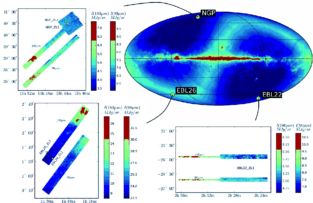 |
Figure B.1:
The ISOPHOT EBL fields. The three frames show the 180 |
| Open with DEXTER | |
B.2 Reduction of EBL field observations
The ISOPHOT data were processed with PIA (PHT Interactive Analysis) program version 11.3. For details of the analysis steps, see the ISOPHOT Handbook (Laureijs et al. 2003) and Appendix, Sect. A. For C100 a method of signal transient correction was introduced in PIA 11.3. This procedure was used for all C100 measurements. Nevertheless, some of the internal calibrator (FCS) measurements show residual drifts. In those cases we applied transient recognition which removes the initial, unstabilised part of the measurements. The flux density calibration was made using the internal calibrator measurements (FCS1) performed immediately before and after each map for actual detector response assessment. The calibration was applied using the average response of the two FCS measurements.
The reduced data contained a few artifacts. These include short time scale detector drifts at the beginning of some C100 observations, temporary signal variations caused by cosmic ray glitches, and occasional drifting of some detector pixels that may also be connected with cosmic ray hits. The time ordered data were examined by eye. For rasters and detector pixels affected by clear anomalies (glitches or drifting) the corresponding PIA error estimates were scaled upwards, typically by a factor of a few. For each detector pixel the signal values were scaled so that their average value over a map became equal to the overall average over all detector pixels. The scaling takes into account the already manually adjusted error estimates. The flat fielding would actually not be necessary, because FIR fluxes are compared only with observed HI 21 cm lines and, therefore, averaged over areas that are large compared with the size of the ISOPHOT rasters.
Long term detector response drifts are not taken out by a simple averaging of the FCS measurements, nor is an initial non-linear drift corrected for by linear interpolation between the two FCS measurements. Both could introduce an artificial gradient in the time ordered data and, because of the systematic scan pattern, also in the maps. The maps were compared with IRAS data in order
to see if there were any gradients uncorrelated with the IRAS 100 ![]() m signal. The only significant difference was found in the C200 observations of the southern NGP field. The gradient was removed while keeping the average surface brightness unchanged. The correction has little effect on the subsequent analysis. Apart from the EBL22 field, all maps contain four detector scans that run alternatively in opposite directions along the longer map dimension. When data are correlated with the lower resolution HI observations, the subsequent scan legs tend to cancel out any long term
drifts.
m signal. The only significant difference was found in the C200 observations of the southern NGP field. The gradient was removed while keeping the average surface brightness unchanged. The correction has little effect on the subsequent analysis. Apart from the EBL22 field, all maps contain four detector scans that run alternatively in opposite directions along the longer map dimension. When data are correlated with the lower resolution HI observations, the subsequent scan legs tend to cancel out any long term
drifts.
The raster map observations themselves do not contain any direct measurement of the dark current. In such cases one usually relies on the orbit dependent ``default'' dark current estimates included in the PIA. However, absolute photometry PHT-25 measurements were carried out within a couple of hours before or after each raster map. The data reduction was carried out also using the dark current and cold FCS values obtained from those measurements. In the subsequent analysis, we use maps that are averages of those obtained using default dark current values and those obtained using PHT-25 dark current measurements.
When absolute photometry points were inside the mapped area they were compared with the surface brightness of the raster maps. The maps were re-scaled so that the final surface brightness corresponds to the average of the original FCS calibrated maps and the values given by the absolute photometry measurements. This causes systematic lowering of the surface brightness values
of the original maps. For EBL26, NGP(N), and NGP(S) the change is typically ![]() 4%, for both C100 and C200 observations. In the case of EBL22 the correction is larger, some 20%, for the C200 detector.
4%, for both C100 and C200 observations. In the case of EBL22 the correction is larger, some 20%, for the C200 detector.
In the region NGP there are separate northern and southern fields that overlap by a few arcminutes. The maps, each containing 32 ![]() 4 raster points, were fitted together using the overlapping area, where the final map is at a level equal to the average of the northern and the southern maps. The resulting change in the surface brightness levels of individual maps was
4 raster points, were fitted together using the overlapping area, where the final map is at a level equal to the average of the northern and the southern maps. The resulting change in the surface brightness levels of individual maps was ![]() 5% or less. In the north there is yet another 15
5% or less. In the north there is yet another 15 ![]() 15 raster map that was observed only at 180
15 raster map that was observed only at 180 ![]() m. Because that measurement includes only very short FCS measurements, it was scaled to fit the already combined long 180
m. Because that measurement includes only very short FCS measurements, it was scaled to fit the already combined long 180 ![]() m map. This required scaling of the surface brightness values by a factor of 1.05.
m map. This required scaling of the surface brightness values by a factor of 1.05.
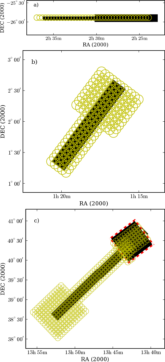 |
Figure B.2:
The figures shows as black rectangles the areas mapped with ISOPHOT (90, 150, and 180 |
| Open with DEXTER | |
The main maps of the field EBL22 cover an area of low cirrus emission. There are additional one-directional scans that extend to a region of higher surface brightness in the west. In the absence of scans in the opposite direction, it is not possible to directly determine the presence of detector response drifts. However, these observations were reduced using the average of the responsivities given by the two FCS measurements and the error bars reflect also the difference in the responsivity before and after the measurement. Using the overlapping area, the 32 ![]() 1 raster strips were scaled to the same level with the 32
1 raster strips were scaled to the same level with the 32 ![]() 3 raster maps. The scalings applied were 0.97, 1.02, and 0.84 at 90
3 raster maps. The scalings applied were 0.97, 1.02, and 0.84 at 90 ![]() m, 150
m, 150 ![]() m, and 180
m, and 180 ![]() m, respectively.
m, respectively.
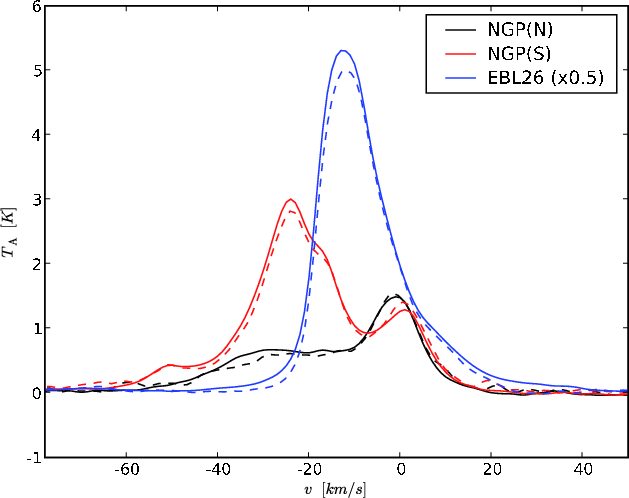 |
Figure B.3:
Comparison of HI spectra from the Leiden/Dwingeloo survey (Kalberla et al. 2005; dashed lines) and our Effelsberg data convolved with a beam of 36
|
| Open with DEXTER | |
The final FIR errorbars show the uncertainty for the weighted means over the Effelsberg beam. The noise of each HI spectrum was estimated separately using the velocity channels outside the line. The uncertainty of the line area was calculated assuming the same, uncorrelated noise for the integrated velocity interval. This might underestimate the total uncertainty, because it ignores the uncertainties in the stray radiation subtraction that do not affect the signal in the line wings. However, for a small field the stray radiation causes a constant systematic error rather than statistical uncertainty and does not affect the weighting of the observations when the linear fit is made.
For selected positions there exist mid-infrared observations made with the ISOPHOT P-detectors as well as further absolute photometry measurements with the C100 and C200 cameras (see Appendix, Table B.2). These observations were performed for the purpose of estimating the zodiacal light. The data reduction of P-detector data is similar to that of the C100 and C200 cameras, except that also signal linearisation is included.
B.3 HI measurements
The observations of the hydrogen 21 cm line were made with the Effelsberg radio telescope in May 2002. The observed positions, 580 in number, are indicated in Fig. B.2. The integration times were 30 s in EBL22 and 62 s in EBL26. In the field NGP the observations were done with 62 s integrations except for the northern part where the integration time was 94 s. The average noise estimated from the velocity intervals outside the HI line is 0.15 K per channel of 1 km s-1. This corresponds to a typical uncertainty of 1.7 K km s-1 in the integrated line area.
For calibration purposes and for precise subtraction of the stray radiation, regular observations of the standard region S7 were made. The stray radiation subtraction is crucial because it affects the zero point of the estimated HI column densities. The observed fields, NGP in particular, have some of the lowest line-of-sight column densities over the whole sky. Under these conditions the stray radiation received by the telescope side lobes becomes a significant fraction of the total signal. The stray radiation was removed with a program developed by Kalberla (Kalberla et al. 2005; see Sect. 3).
In Fig. B.3 we compare our data with spectra from the Leiden/Dwingeloo survey (Hartmann & Burton 1997; Kalberla et al. 2005). For this comparison, in order to match the resolution of the Leiden/Dwingeloo survey, the Effelsberg data were convolved
with a Gaussian with FWHM equal to 36
![]() .
The HI profiles agree very well. Part of the differences may be caused by the fact that our HI maps do not cover the whole area of the 36
.
The HI profiles agree very well. Part of the differences may be caused by the fact that our HI maps do not cover the whole area of the 36
![]() beams. Nevertheless, the figure shows that the observations and the stray radiation subtraction (see Sect. 3) are consistent with the Kalberla (2005)
results.
beams. Nevertheless, the figure shows that the observations and the stray radiation subtraction (see Sect. 3) are consistent with the Kalberla (2005)
results.
Appendix C: Calibration accuracy
The error estimates listed in Table 1 are based on the statistical uncertainties in the fits between FIR and HI data. The scatter of data points around the fitted lines is usually larger than their estimated uncertainty. This could be a sign of underestimated measurement uncertainties but is more likely caused by true scatter in the relation. If the formal uncertainties of the line parameters were estimated based on the error estimates of the individual points, the uncertainties could be severely underestimated. Therefore, instead of relying only on the measurement uncertainties, the uncertainty of the fit parameters was estimated separately with the bootstrap method so that they reflect the true scatter of observed points. The error estimates corresponding to a 67% confidence interval are given in Table 1.
These uncertainties do not include estimates for the systematic errors introduced by the independent calibration of each map or the absolute accuracy of the overall ISOPHOT calibration. There are both multiplicative and additive sources of uncertainty. The former include, for example, uncertainties in the internal calibration source (FCS) measurements (e.g., detector drifts) that alter the estimated detector response. The uncertainties that affect the zero point of the intensity scale are more critical, because the CIRB is small compared with the observed signal and can be recovered only as the residual after the subtraction of the ZL.
Table C.1 lists an assessment of uncertainty that, using data in Table 1, have been converted into uncertainty of the FIR flux at zero HI column density. The quoted values are half of the difference of two values obtained in two independent ways. Thereby the quoted values are also ![]() 1-
1-![]() estimates for the uncertainty of the average of the two values.
estimates for the uncertainty of the average of the two values.
In Table C.1 Col. 4 has been obtained by comparing the fine calibration source measurements performed before and after each map. The numbers indicate the statistical uncertainty of the detector response measurements. The FCS measurements are generally very consistent, particularly in the case of the C200 detector. On the other hand, the effect of the drift affecting the first FCS measurement of the one-dimensional strip map of EBL22 is clearly visible at 90 ![]() m.
m.
The dark signal subtraction is the most important correction affecting the zero point of the FIR intensity. Close to each of the raster map observations, we have one or two absolute photometry observations which include dark signal measurements of their own. In PIA, the default dark current calibration is based on a larger set (![]() 70) of dark current measurements for which the
orbit trend has been determined. Therefore, the PIA default dark current calibration is less affected by the noise of individual measurements but may not take into account short time scale variations in the detector dark current on a specific orbit. The maps were reduced using the default dark current values and the actually measured dark current values. In Table C.1 Col. 5 shows the associated uncertainty in the FIR signal at zero HI column density. The observed uncertainty in the dark current values is comparable with the
variation observed in the systematic analysis of a large sample of ISOPHOT observations (del Burgo et al. 2002; see also Fig. A.5).
70) of dark current measurements for which the
orbit trend has been determined. Therefore, the PIA default dark current calibration is less affected by the noise of individual measurements but may not take into account short time scale variations in the detector dark current on a specific orbit. The maps were reduced using the default dark current values and the actually measured dark current values. In Table C.1 Col. 5 shows the associated uncertainty in the FIR signal at zero HI column density. The observed uncertainty in the dark current values is comparable with the
variation observed in the systematic analysis of a large sample of ISOPHOT observations (del Burgo et al. 2002; see also Fig. A.5).
When absolute photometry measurements existed within mapped areas, those were used to re-scale the surface brightness values of the maps (see Sect. B.2). The difference in the absolute photometry and mapping measurements is used to derive the values in Col. 6 of Table C.1. The final column reflects the difference in the surface brightness in areas where two independently calibrated maps overlap. The numbers in Cols. 6 and 7 include, of course, dark current and FCS uncertainties as one of their components. For the C100 observations at 90 ![]() m the uncertainty is close to 1 MJy sr-1, i.e., comparable with the expected EBL signal. On the other hand, for the C200 detector the uncertainty of an individual map is
m the uncertainty is close to 1 MJy sr-1, i.e., comparable with the expected EBL signal. On the other hand, for the C200 detector the uncertainty of an individual map is
![]() 0.3 MJy sr-1. Most of this is caused by the uncertainty in the dark current values.
0.3 MJy sr-1. Most of this is caused by the uncertainty in the dark current values.
Table C.1: Assessment of the calibration uncertainty for the ISOPHOT maps. Columns are (1) name of the field; (2) wavelength; (3) average surface brightness of the map; (4) difference between calibration measurements performed before and after each map; (5) difference between actual dark current measurements and default dark current values; (6) difference between the independently calibrated absolute photometry measurements and raster maps; and (7) difference between partially overlapping maps. These uncertainties have been converted to correspond to the uncertainties at zero hydrogen column density using the fit parameters listed in Table 1.
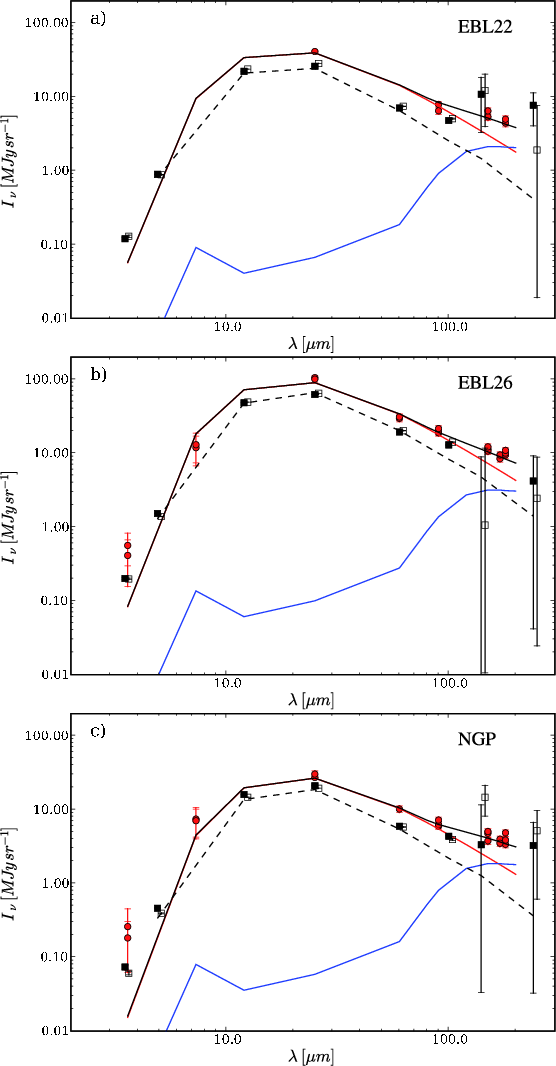 |
Figure C.1: Fits used to estimate the ZL levels in the three fields EBL22, EBL26, and NGP (frames a)- c), respectively). The red circles are ISOPHOT observations. The lower lines are the cirrus (blue solid line) and the ZL (red solid line) templates, the uppermost solid green line is their sum. The figures also show DIRBE values for the closest DIRBE pixel, read from the DIRBE weekly maps. The solid squares correspond to observations with the same solar elongation as in the case of ISOPHOT observations, the open squares to the other measurement with identical absolute value of the solar aspect angle but opposite solar elongation. For clarity, the latter have been shifted slightly in wavelength. The dashed line shows the predictions of the Kelsall et al. (1998) ZL model. |
| Open with DEXTER | |
C.1 Straylight radiation
Straylight may be another instrumental artefact affecting the zero level of the FIR surface brightness. By design and operation ISO's viewing direction stayed by several tens of degrees away from the brightest FIR emitters in the sky, the Sun, the Earth and the Moon (Kessler et al. 2003). A dedicated straylight program was executed verifying by deep ``differential'' integrations that the uniform straylight level due to these sources was below ISOPHOT's detection limit, even under the most unfavourable pointing conditions close to the visibility constraints (Lemke et al. 2001).
Specular straylight by the second brightest class of objects, the giant planets Jupiter and Saturn, was observed when pointing to within 15
![]() to 1
to 1
![]() of the planet, expressing itself as finger-like stripes or faint ghost rings (Kessler et al. 2003; Lemke et al.
2001). The NGP and EBL 22 fields are far away from the ecliptic and can thus not suffer from this type of straylight. For EBL 26 we checked the positions of the planets Mars, Jupiter, Saturn, Uranus and Neptune at the time of the observations, 1997-06-26 and 1997-07-11, respectively. Mars, Jupiter, Uranus, Neptune were all far off. Saturn was at a distance of 3.25 degrees, which is still more than a factor of 3 off of any known straylight-critical distance.
of the planet, expressing itself as finger-like stripes or faint ghost rings (Kessler et al. 2003; Lemke et al.
2001). The NGP and EBL 22 fields are far away from the ecliptic and can thus not suffer from this type of straylight. For EBL 26 we checked the positions of the planets Mars, Jupiter, Saturn, Uranus and Neptune at the time of the observations, 1997-06-26 and 1997-07-11, respectively. Mars, Jupiter, Uranus, Neptune were all far off. Saturn was at a distance of 3.25 degrees, which is still more than a factor of 3 off of any known straylight-critical distance.
Appendix D: Determination of the ZL levels
The ZL level was estimated by fitting ZL and cirrus templates to ISOPHOT observations in the wavelength range from 7.3 ![]() m to 200
m to 200 ![]() m (see Sect. 4.2). Figure C.1 shows the results of these fits. In the field EBL22 we had observations of one position and in the fields EBL26 and NGP of two positions (see Table B.2). For the latter two fields, the figures show the fit to data combined from the two positions.
m (see Sect. 4.2). Figure C.1 shows the results of these fits. In the field EBL22 we had observations of one position and in the fields EBL26 and NGP of two positions (see Table B.2). For the latter two fields, the figures show the fit to data combined from the two positions.
Table B.2 lists the time difference between the listed observations and the observations of the raster maps. In the case of NGP these are relative to the 150 ![]() m observations. The 90
m observations. The 90 ![]() m maps were observed four days before and the 180
m maps were observed four days before and the 180 ![]() m one day after the 150
m one day after the 150 ![]() m maps. According to the Kelsall et al. (1998) ZL model the four day difference causes only
m maps. According to the Kelsall et al. (1998) ZL model the four day difference causes only ![]() 1.5% change in the expected ZL. The combined NGP map is almost 1.5 degrees long. In the Kelsall model the difference in the centre positions of the southern and northern parts corresponds to about 1% difference in the ZL. Therefore, we use only one zodiacal estimate value for both NGP(N) and NGP(S) and for all observations made during the five day interval.
1.5% change in the expected ZL. The combined NGP map is almost 1.5 degrees long. In the Kelsall model the difference in the centre positions of the southern and northern parts corresponds to about 1% difference in the ZL. Therefore, we use only one zodiacal estimate value for both NGP(N) and NGP(S) and for all observations made during the five day interval.
In the fields EBL26 and NGP, MIR observations exist for two separate positions (see Fig. B.1). In both fields, the measurements at these two positions are close to each other, both in time and position. Therefore, their ZL values should be identical and also the cirrus levels should be very similar. Comparison of the fits performed using these independent sets of measurements gives the first indication of the statistical uncertainty of the ZL values. In both fields, the ZL values obtained for the two positions agree within 10%.
The observations are fitted as a sum of ZL and cirrus components. The ZL template is a black body curve at the temperature obtained from Leinert et al. (2002). The cirrus template is based on the model by Li & Draine (2001). Using the ISOPHOT filter profiles we calculate for both radiation components, ZL and cirrus, and for each filter the in-band power values that can be directly compared with the observed values. In the fit we have only two free parameters, the intensity of the ZL component and the intensity of the cirrus component. The ZL estimates should be based mainly on data between 10 ![]() m and 60
m and 60 ![]() m where the ZL is clearly the dominant
component. Therefore, in the fit, the weight of the data points in this
wavelength range is increased by a factor of two.
m where the ZL is clearly the dominant
component. Therefore, in the fit, the weight of the data points in this
wavelength range is increased by a factor of two.
The level of the cirrus component is determined mostly by the longer wavelength data. In reality, the component corresponds to the sum of the cirrus and CIRB signals. As long as the component is small in the MIR, the ZL estimates are almost independent of the exact shape of this template. We confirmed this by replacing the Li & Draine (2001) cirrus template by a pure CIRB template, using the model curve from Dole et al. (2006; Fig. 13). The resulting change in the ZL estimates was less than one per cent.
The actual statistical errors of the ZL values are estimated using the standard deviation of the relative errors when observations are compared with the fitted ZL curve. The last column of Table 2 lists the corresponding error of the mean, calculated using data points between 7.3 ![]() m and 90
m and 90 ![]() m. In the case of fields NGP and EBL26, the error estimates are calculated from the fits where we have combined the data from the two measured positions within each field. In all three fields, the obtained relative uncertainties are
m. In the case of fields NGP and EBL26, the error estimates are calculated from the fits where we have combined the data from the two measured positions within each field. In all three fields, the obtained relative uncertainties are ![]() 10%. In the fields EBL26 and NGP the uncertainties are also consistent with the difference of the ZL values obtained for the two individual positions. The ZL fits are shown in Fig. C.1.
10%. In the fields EBL26 and NGP the uncertainties are also consistent with the difference of the ZL values obtained for the two individual positions. The ZL fits are shown in Fig. C.1.
In this paper we have used original ISOPHOT observations without applying colour corrections. Therefore, in the fitting procedure also the ZL and cirrus templates were converted to corresponding values using the ISOPHOT filter profiles. However, for Fig. C.1 we have performed colour
corrections. The templates are plotted by connecting the values at the nominal wavelengths by a straight line. The template spectra used in the ZL fitting are colour corrected using their respective spectral shapes. In the figure, the colour correction of the observed surface brightness values is done assuming the blackbody ZL spectrum below 90 ![]() m, and a modified black body
cirrus spectrum,
m, and a modified black body
cirrus spectrum,
![]() ,
at 90
,
at 90 ![]() m and longer wavelengths.
m and longer wavelengths.
The plots include DIRBE values from the DIRBE weekly maps. These correspond to the DIRBE pixel closest to the centre of the corresponding ISOPHOT map. Linear interpolation was performed between the weeks in order to accurately match the solar elongation of the ISOPHOT observations. In addition to the DIRBE value that corresponds directly to the ISOPHOT observations (solid squares) we plot the DIRBE value for the same solar aspect angle and opposite sign of the solar elongation. Assuming that the zodiacal dust cloud is symmetric along the ecliptic, the two values should be identical. The
predictions of the ZL model of Kelsall et al. (1998) are also plotted. The DIRBE values are colour corrected. As in the case of ISOPHOT data, colour correction of the observations assumes a blackbody ZL spectrum at and below 60 ![]() m, and a modified black body cirrus spectrum,
m, and a modified black body cirrus spectrum,
![]() ,
at the longer wavelengths, 100, 140, and 240
,
at the longer wavelengths, 100, 140, and 240 ![]() m.
m.
There is a clear difference in the ISOPHOT and DIRBE surface brightness scales. The DIRBE values are consistently lower by some 20-30%, in the MIR range. In the FIR bands the extended cirrus structures combined with the much larger pixel size and noise in the DIRBE pixels precludes direct comparison. The determination of the CIRB values is not directly affected by a possible calibration difference between DIRBE and ISOPHOT because, in this paper, we use exclusively ISOPHOT measurements.
Systematic uncertainties affecting all ISOPHOT bands have only little impact on the derived CIRB values. The relative calibration accuracy between the FIR cameras and the ISOPHOT-P photometer is more important, because the zodiacal light estimates are based on the latter. When the absolute level of the zodiacal light was estimated we calculated the scatter between the SED model and the observations at different wavelengths (see Table 2). The scatter was typically ![]() 10-20%. The importance of this error source depends, of course, on the absolute level of the ZL emission. The field EBL26 is located near the ecliptic plane and at 90
10-20%. The importance of this error source depends, of course, on the absolute level of the ZL emission. The field EBL26 is located near the ecliptic plane and at 90 ![]() m the observed signal and the ZL are both of the order of 20 MJy sr-1. Therefore, a relative uncertainty of 10% would already correspond to about twice the expected level of the CIRB. For EBL22 and especially for NGP the zodiacal light level is much lower so that more meaningful limits can be derived for the CIRB also at 90
m the observed signal and the ZL are both of the order of 20 MJy sr-1. Therefore, a relative uncertainty of 10% would already correspond to about twice the expected level of the CIRB. For EBL22 and especially for NGP the zodiacal light level is much lower so that more meaningful limits can be derived for the CIRB also at 90 ![]() m.
m.
The quoted ZL error estimates reflect the uncertainty in the determined ZL level in the mid-infrared. If there were a systematic difference in the calibration of the mid- and FIR-bands, the ZL estimates could be wrong by the corresponding amount. Generally the relative calibration accuracy is considered to be within 15%. This uncertainty would not necessarily be reflected in the quality of the ZL spectrum fits, because a systematic calibration error could have been partly compensated by a change in the intensity of the cirrus component.
The ZL spectrum was assumed to be a pure black body with the temperature given by Leinert et al. (2002). As far as the mid-infrared points are concerned, a wrong temperature would, at some level, be reflected also in our error estimate. However, if the ZL spectrum deviated from the assumed shape only in the FIR this could again be masked by a change in the fitted cirrus component without a corresponding increase in the rms value. Therefore, we must explicitly assume that the same ZL temperature is applicable both at mid-infrared and far-infrared wavelengths. However, because a 5 K change in the ZL temperature corresponds to only ![]() 2% relative change in the ratio of 150
2% relative change in the ratio of 150 ![]() m and 25
m and 25 ![]() m intensities, this source of uncertainty is unimportant compared with the uncertainty in the relative calibrations of the different detectors.
m intensities, this source of uncertainty is unimportant compared with the uncertainty in the relative calibrations of the different detectors.
Appendix E: Comparison with DIRBE EBL estimates
This present study represents the first determination of the absolute level of the FIR EBL that is independent of measurements of the COBE DIRBE instrument. In Table E.1 we list FIR EBL estimates given in seven publications based on the DIRBE measurements. Included are also our
2-![]() upper limit at 90
upper limit at 90 ![]() m and the EBL estimate for the range 150-180
m and the EBL estimate for the range 150-180 ![]() m.
m.
Table E.1: Comparison of existing CIRB estimates in the FIR range. The error estimates quoted by the authors are shown in parenthesis. In our case, we include only the statistical uncertainty.
Footnotes
- ... instrument
- Based on observations with the Infrared Space Observatory ISO. ISO is an ESA project with instruments funded by ESA member states (especially the PI countries France, Germany, The Netherlands, and the UK) and with participation of ISAS and NASA.
- ...
- Appendices are only available in electronic form at http://www.aanda.org
All Tables
Table 1: Parameters of linear fits of FIR surface brightness versus the HI line area.
Table 2: The estimated zodiacal light emission.
Table 3: Estimated level of the CIRB for the individual fields.
Table A.1:
Effective solid angles for the 3 ![]() 3 pixels of ISOPHOT's C100 array for the 6 filters with central wavelengths
3 pixels of ISOPHOT's C100 array for the 6 filters with central wavelengths
![]() .
.
Table A.2:
Effective solid angles for the 2 ![]() 2 pixels of ISOPHOT's C200 array for the 5 filters with central wavelengths
2 pixels of ISOPHOT's C200 array for the 5 filters with central wavelengths
![]() .
.
Table B.1: List of ISOPHOT observations of EBL fields carried out in the PHT-22 and PHT-25 observation modes.
Table B.2:
Observations used for the determination of the zodiacal light emission. The columns are: (1) name of the field; (2), (3) position; (4) wavelength; (5) the ISO identifier number (TDT) of the observation; and (6) time difference between the listed observation and the observation of the EBL raster maps of Table B.1. A time difference is quoted only when the observations were not performed within the same day. Observations at wavelengths below 60 ![]() m are made with the ISOPHOT-P detector.
m are made with the ISOPHOT-P detector.
Table B.3:
The positions and sizes of the observed fields. Columns are: (1) name
of the field; (2), (3) equatorial coordinates of the centre of the field; (4), (5) galactic coordinates; (6), (7) ecliptic coordinates; (8) number of raster points; (9) area in square degrees; and (10) additional remarks. All areas were observed at 90, 150, and 180 ![]() m. In NGP(N) an additional square map was observed at 180
m. In NGP(N) an additional square map was observed at 180 ![]() m only. Details of the individual measurements are listed in Appendix, in Table B.1.
m only. Details of the individual measurements are listed in Appendix, in Table B.1.
Table C.1: Assessment of the calibration uncertainty for the ISOPHOT maps. Columns are (1) name of the field; (2) wavelength; (3) average surface brightness of the map; (4) difference between calibration measurements performed before and after each map; (5) difference between actual dark current measurements and default dark current values; (6) difference between the independently calibrated absolute photometry measurements and raster maps; and (7) difference between partially overlapping maps. These uncertainties have been converted to correspond to the uncertainties at zero hydrogen column density using the fit parameters listed in Table 1.
Table E.1: Comparison of existing CIRB estimates in the FIR range. The error estimates quoted by the authors are shown in parenthesis. In our case, we include only the statistical uncertainty.
All Figures
| |
Figure 1:
FIR surface brightness as a function of HI line area W(HI) in the three EBL fields, EBL22 ( left), EBL26 ( middle), and NGP ( right). Each point
corresponds to one pointing of the HI observations. The uncertainties in the HI line area are estimated based on the noise in velocity channels outside detected HI emission. For each HI spectrum the corresponding average FIR signal has been calculated using for weighting a Gaussian with FWHM = 9
|
| Open with DEXTER | |
| In the text | |
| |
Figure A.1:
Synthetic (outer part, i.e. green and blue coloured areas, modelled) footprints (convolution of the ISO telescope PSF with the pixel aperture response) of the 3 |
| Open with DEXTER | |
| In the text | |
| |
Figure A.2: Scheme of the ISOPHOT calibration steps associated with the different instrument components. The meaning of the abbreviations is the following: BSL = Bypassing Sky Light correction, DS = detector Dark Signal, RL = Ramp Linearisation, TC = signal Transient Correction, and RIC = Reset Interval Correction. |
| Open with DEXTER | |
| In the text | |
| |
Figure A.3: Steps in the generation of a homogeneous and most complete calibration of ISOPHOT's long wavelength internal calibration sources (FCS). This is illustrated for the central pixel (#5) of the C100 array camera. Upper left: measured relation between optical power received on the detector and the heating power applied to the internal source. Dots indicate the discrete measurements, the solid line is a fit. Upper right: display of the input curves for all C100 filters within the reliable heating power range. Middle left: for a selected heating power (here: 1.0 mW) monochromatic and colour corrected fluxes of all filters are fitted by a modified BB curve. Middle right: by repeating the fits with the same modified BB type for the whole heating power range covered the relation between heating power and temperature of the internal source is established. Lower centre: by applying the FCS model the relation between optical power and heating power is homogenized and extended to the maximum heating power range covered by at least one measurement in any of the C100 or C200 filters. |
| Open with DEXTER | |
| In the text | |
| |
Figure A.4: Bypassing sky light contribution to the FCS signal depending on the sky background. |
| Open with DEXTER | |
| In the text | |
| |
Figure A.5: Orbit dependent dark signal determination for the central pixel 5 of ISOPHOT's C100 array. Dots represent individual measurements obtained during the entire ISO mission, filled and open signals identify a different reset interval in the integration of the dark signal. The solid line is the fit to the measurements providing the so-called default dark level. The dotted line is the default dark level of an older calibration version used before 2001. |
| Open with DEXTER | |
| In the text | |
| |
Figure A.6: Correction of the signal dependence on the selected reset interval. Upper panel: demonstration of the effect, showing the resulting signal versus the selected reset interval over the range from 1/32 s up to 8 s (reset intervals were commanded in powers of 2) under constant illumination. Middle panel: solid line: correction relation for a reset interval of 8 s w.r.t. the reference reset interval of 1/4 s for all C100 array pixels, except the ones on the main diagonal. Dotted line: old linear correlation used before the re-analysis. Lower panel: solid line: Correction relation for a reset interval of 8 s w.r.t. the reference reset interval of 1/4 s for all C100 array pixels on the main diagonal (pixels #1, 5, and 9). Dotted line: old linear correlation used before the re-analysis (same as for middle panel). |
| Open with DEXTER | |
| In the text | |
| |
Figure A.7: Empirical signal transient correction for ISOPHOT's C100 array. The left column shows the signal loss for integration times of 4, 8, 16, 32, and 64 s (commendable integration times of ISOPHOT detectors) with regard to the reference time of 128 s. The red line is a fit through the measured points over the covered signal range and is used as the correction relation. The right column shows the residuals after applying this correction. |
| Open with DEXTER | |
| In the text | |
| |
Figure B.1:
The ISOPHOT EBL fields. The three frames show the 180 |
| Open with DEXTER | |
| In the text | |
| |
Figure B.2:
The figures shows as black rectangles the areas mapped with ISOPHOT (90, 150, and 180 |
| Open with DEXTER | |
| In the text | |
| |
Figure B.3:
Comparison of HI spectra from the Leiden/Dwingeloo survey (Kalberla et al. 2005; dashed lines) and our Effelsberg data convolved with a beam of 36
|
| Open with DEXTER | |
| In the text | |
| |
Figure C.1: Fits used to estimate the ZL levels in the three fields EBL22, EBL26, and NGP (frames a)- c), respectively). The red circles are ISOPHOT observations. The lower lines are the cirrus (blue solid line) and the ZL (red solid line) templates, the uppermost solid green line is their sum. The figures also show DIRBE values for the closest DIRBE pixel, read from the DIRBE weekly maps. The solid squares correspond to observations with the same solar elongation as in the case of ISOPHOT observations, the open squares to the other measurement with identical absolute value of the solar aspect angle but opposite solar elongation. For clarity, the latter have been shifted slightly in wavelength. The dashed line shows the predictions of the Kelsall et al. (1998) ZL model. |
| Open with DEXTER | |
| In the text | |
Copyright ESO 2009
Current usage metrics show cumulative count of Article Views (full-text article views including HTML views, PDF and ePub downloads, according to the available data) and Abstracts Views on Vision4Press platform.
Data correspond to usage on the plateform after 2015. The current usage metrics is available 48-96 hours after online publication and is updated daily on week days.
Initial download of the metrics may take a while.