| Issue |
A&A
Volume 499, Number 2, May IV 2009
|
|
|---|---|---|
| Page(s) | 601 - 613 | |
| Section | Planets and planetary systems | |
| DOI | https://doi.org/10.1051/0004-6361/200811213 | |
| Published online | 05 March 2009 | |
Detection of real periodicity in the terrestrial impact crater record: quantity and quality requirements
J. Lyytinen - L. Jetsu - P. Kajatkari - S. Porceddu
Observatory, PO Box 14, 00014 University of Helsinki, Finland
Received 22 October 2008 / Accepted 30 January 2009
Abstract
Aims. To determine the quantity and quality requirements for the terrestrial impact crater data which would allow reliable detection of real periodicity.
Methods. Artificial impact crater data samples of different size and accuracy are simulated. Erosion is considered, as well as the effect of the unknown ratio between periodic and aperiodic impacts. The probabilities for detecting real and false periodicities are solved with the Rayleigh test from these simulated data.
Results. Reliable detection of real periodicity is currently impossible - unless all impacts on Earth have been periodic.
Key words: Earth - minor planets, asteroids - Oort cloud - methods: statistical - Galaxy: solar neighborhood - comets: general
1 Introduction
Alvarez & Muller (1984) detected a 28.4 Myr periodicity in the ages of terrestrial impact craters. In the same volume of Nature, two theories on the possible astronomical process capable of triggering periodic comet showers from the Oort cloud were presented. Davis et al. (1984) and Whitmire & Jackson (1984) suggested that an unseen solar companion ``Nemesis'' causes periodic perturbances to the Oort cloud, and Rampino & Stothers (1984) and Schwartz & James (1984) argued for perturbances caused by the oscillation of the Solar System through the Galactic plane. For a quarter of a century, evidence that confirms the existence of real periodicity in these catastrophic events has been published, e.g. by Stothers (1998), Moon et al. (2003), Yabushita (2004), Chang & Moon (2005), Stothers (2006) and Wickramasinghe & Napier (2008). Evidence against such periodicity has also been presented, e.g. by Bailey & Stagg (1988), Grieve et al. (1988), Deutsch & Schaerer (1994), Grieve & Pesonen (1996), Jetsu (1997) and Jetsu & Pelt (2000).
We decided to determine the quantity and quality requirements for the terrestrial impact crater data that would allow reliable detection of real periodicity, if present. We also noted the presence of erosion and different values for the ratio between periodic and aperiodic impacts.
2 Real data
2.1 Detection rate
Several geological processes reduce the detectability of terrestrial impact craters as a function of time. This decrease in detectability was estimated from the crater data in The Earth Impact Database![]() maintained by the Planetary and Space Science Centre at the University of New Brunswick. These data contained n=174 impact structures. The errors for the ages were available for n=89 craters. Simultaneous pairs of events were combined as in Jetsu (1997). As in that particular study, the age
maintained by the Planetary and Space Science Centre at the University of New Brunswick. These data contained n=174 impact structures. The errors for the ages were available for n=89 craters. Simultaneous pairs of events were combined as in Jetsu (1997). As in that particular study, the age
![]() [Myr] and the diameter Di [km] of each crater were then used for selecting the two subsamples of data:
[Myr] and the diameter Di [km] of each crater were then used for selecting the two subsamples of data:

These data are given in Table 1. It contains the following information for each crater: name (Col. 1), location (Col. 2), age (Col. 3), diameter (Col. 4), belongs (``Yes'') or does not belong (``No'') to the sub-sample C2 or C3 (Cols. 5 and 6), and the cycle number ki=1, 2, ..., 10 in C2 and C3 (Cols. 7 and 8). For each ti, this cycle number is
Table 1:
The most recent terrestrial impact crater data obtained in August 11th, 2008 from The Earth Impact Database. The combined simultaneous pairs of impacts are marked with ``![]() ''. The following information of these craters is given: name (Col. 1), location (Col. 2), age and its error (Col. 3:
''. The following information of these craters is given: name (Col. 1), location (Col. 2), age and its error (Col. 3:
![]() ), diameter (Col. 4:
), diameter (Col. 4:
![]() )
and the crater belongs (``Yes'') or does not belong (``No'') to the sub-sample C2 or C3 (Cols. 5 and 6). The value of ki is the cycle number in C2 and C3 (Cols. 7 and 8).
)
and the crater belongs (``Yes'') or does not belong (``No'') to the sub-sample C2 or C3 (Cols. 5 and 6). The value of ki is the cycle number in C2 and C3 (Cols. 7 and 8).
2.2 Age uncertainty
Table 2: The fractional crater detectability estimates calculated from data of Table 1: Col. 1 (k) is the cycle number. Columns 2 (a1) and 3 (a2) give the number of craters within cycle k divided by the total number of craters in samples C2(n=33) and C3(n=40). Columns 4 (a3) and 5 (a4) give the averages for pairs of two consecutive cycles in samples C2 and C3. Column 6 ( Ak=(a3+a4)/2) is the mean of both samples.
For K cycles of equal length over the whole time span of the data
![]() ,
the period is
PK = (tn- t1)/K.
Our definition for the average error of these data is
,
the period is
PK = (tn- t1)/K.
Our definition for the average error of these data is

where
where
2.3 Origin of periodicity
The periodicity detected by Alvarez & Muller (1984) in the terrestrial impact crater record has been suggested to be caused by regular ``comet showers'' from the Oort cloud towards the inner solar system (Davis et al. 1984; Whitmire & Jackson 1984; Rampino & Stothers 1984; Schwartz & James 1984). However, direct evidence for such comet showers is lacking. Although Farley (1998) argued for a cometary shower hitting the Earth 35 Myr ago, his findings have been disputed by Tagle & Claeys (2004).
Since 1984, the proposed periodicities for the comet showers have ranged between 20 and 40 Myr. Hills (1981), among others, has shown that a comet survives less than 1 Myr in the inner Solar System. Each aforementioned comet shower could therefore be considered as ``an instantaneous event'' in the simulation of the periodic part in Sect. 3.1. Finally, we emphasize that no evidence have been presented for all comet impacts on Earth having been periodic.
2.4 Origin of aperiodicity
According to Neukum & Ivanov (1994), the impact cratering rate of the Earth-Moon system has been nearly constant for approximately 3 billion years. Gladman et al. (1997) have described how collisions in the main-asteroid-belt can eventually transport asteroids to Earth-crossing orbits. Some fragments of these colliding bodies drift into the gravitational resonance areas of the belt, where their orbits decay into planet-crossing orbits. Vokrouhlicky & Farinella (2000) and Bottke et al. (2002a) have shown how the combination of the Yarkovski effect and the aforementioned collisional dynamics cause a continuous drift of objects from the main-asteroid-belt. Thus the observed Near Earth Object (NEO) population would consist mainly of former main-asteroid-belt objects, but some NEOs might also be ancient comet nuclei. In short, the currently known physical processes indicate that all asteroid impacts on Earth have been aperiodic.
![\begin{figure}
\par\includegraphics[width=7cm,clip]{1213fig1.ps}
\end{figure}](/articles/aa/full_html/2009/20/aa11213-08/img78.png) |
Figure 1:
The simulated case with S=1/3 and
|
| Open with DEXTER | |
3 Simulated data
In this section, we will formulate the simulation of a fully periodic case (Sect. 3.1) and a fully aperiodic case (Sect. 3.2), as well as their combination (Sect. 3.3).
3.1 Periodic component
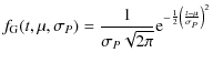
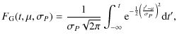
In the fully periodic case we assumed that periodic comet showers have occurred and simulated K=10 such showers at the epochs tk=k-1/2, where k=1,2,...,K. It was assumed that the duration of each comet shower is much shorter than the period PK=P=1 and can be approximated with the Dirac delta function. This gave the probability density and the cumulative distribution functions
These forms represent the convolution of the Gaussian error (Eqs. (2) and (3)) with a Dirac delta function at each tk. The multipliers Ak ensured that
3.2 Aperiodic component
In the fully aperiodic case, we first defined the following probability density function

Again, the Ak values were used to represent the fraction of craters detected within the kth cycle in this aperiodic case (i.e. uniform distribution within each cycle) and to ensure that

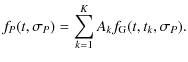
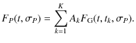
The convolution of f2(t) and F2(t) with the Gaussian error (Eqs. (2) and (3)) gave the following probability density and cumulative distribution functions
![$\displaystyle f_{{\rm A}}(t,\sigma_{{{P}}}) = \sum_{{{k=1}}}^{{{K}}} {A_{{k}}}
...
...[
F_{{\rm G}} (t,k-1,\sigma_{{{P}}}) - F_{{\rm G}} (t,k,\sigma_{{{P}}})
\right]$](/articles/aa/full_html/2009/20/aa11213-08/img87.png)
where the subscript ``A'' in
3.3 Combined components
Finally, the combination of the periodic and aperiodic cases was simulated with the functions
where the constant
In this paper, we have simulated the cases S=0 (fully periodic), S=1/3 or 2/3 (partly periodic) and S=1 (fully aperiodic). For all these S values, all combinations of
n=10, 25, 50, 75, 100 or 200 and
![]() or 0.3 were simulated. The simulation process was simple. First the values of n,
or 0.3 were simulated. The simulation process was simple. First the values of n,
![]() and S were fixed. Then a series of
x1, x2,.., xn random numbers were generated from an uniform distribution [0,1). Finally, the cumulative distribution function was used to solve the simulated data values
and S were fixed. Then a series of
x1, x2,.., xn random numbers were generated from an uniform distribution [0,1). Finally, the cumulative distribution function was used to solve the simulated data values
![]() ,
which fulfilled the relation
,
which fulfilled the relation
![]() .
Note that these simulated
.
Note that these simulated
![]() data and their error
data and their error
![]() were both measured in the units of P=1.
were both measured in the units of P=1.
4 Rayleigh test
The Rayleigh test is formulated as in Jetsu & Pelt (2000). The phases for the time points
![]() are
are
![\begin{eqnarray*}\phi_{{i}} = {{\rm FRAC}}[(t_{{i}}-t_0)P^{-1}] = {{\rm FRAC}}[(t_{{i}}-t_0)f],
\end{eqnarray*}](/articles/aa/full_html/2009/20/aa11213-08/img105.png)
where
H0: ``the phasesThe Rayleigh test statistic iscalculated with an arbitrary tested period P have a random distribution between [0,1)''.
![\begin{displaymath}%
z(f)=\frac{1}{n} \left[
\left( \sum_{{{i=1}}}^{{{n}}} \cos...
...t( \sum_{{{i=1}}}^{{{n}}} \sin \theta_{{i}} \right)^2 \right],
\end{displaymath}](/articles/aa/full_html/2009/20/aa11213-08/img108.png)
where
This parameter Q is hereafter called the critical level. The null hypothesis H0 was rejected if, and only if
where
The best period
![]() for each simulated data sample
for each simulated data sample
![]() was determined from the highest peak of the periodogram,
was determined from the highest peak of the periodogram,
![]() .
In all our tests for the simulated data, only the
.
In all our tests for the simulated data, only the
![]() values between
values between
![]() and
and
![]() were accepted, which prevented the ``detection'' of possibly false
were accepted, which prevented the ``detection'' of possibly false
![]() values outside the tested range
values outside the tested range
![]() .
.
Table 3:
Results of the fully aperiodic simulations for the preassigned significance levels
![]() and 0.001.
and 0.001.
Table 4: The results of the fully periodic (S=0) simulations.
Table 5: Simulation results for the partly periodic cases (S=1/3), otherwise as in Table 4.
Table 6: Simulation results for the partly periodic cases (S=2 / 3), otherwise as in Table 4.
5 Rayleigh test for the simulated data
The fully aperiodic simulations (S=1) are discussed in Sect. 5.1. The fully periodic (S=0) and the partly periodic (S=1/3 and 2/3) simulations are discussed in Sect. 5.2.
5.1 Aperiodic cases (S = 1)
The statistics of the Rayleigh test were based on the ``null hypothesis'' H0 formulated in Sect. 4. There would have been no reason to suspect these statistics if the detectability of the craters had remained constant in our data. Since, however, the detectability of older craters is lower, the statistics based on H0 are not necessarily valid. To study this question, we performed simulations of fully aperiodic cases (S=1 in Eq. (9)), where the Ak values were used to simulate this detectability effect. The Rayleigh test statistics based on the following four fully aperiodic hypotheses
H1: ``the cumulative distribution function for the time points ti iswere simulated for the sample sizes n=10, 25, 50, 75, 100 and 200. Under each hypothesis H1, H2, H3 or H4, we performed the Rayleigh test for Z=100 000 random samples of''. H2: ``the cumulative distribution function for the time points ti is
''. H3: ``the cumulative distribution function for the time points ti is
''. H4: ``the cumulative distribution function for the time points ti is
''.
![\begin{figure}
\par\includegraphics[width=8.8cm,clip]{1213fig2.ps}
\end{figure}](/articles/aa/full_html/2009/20/aa11213-08/img148.png) |
Figure 2:
One arbitrary random sample
|
| Open with DEXTER | |
5.2 Periodic cases (S = 0, 1/3 and 2/3)
In this section, we determine how often the Rayleigh test detects
the ``real'' (P=1) or the ``false''
period (![]() )
in the simulated crater data.
The probability for the ``reliable'' detection of the ``real'' period
is also investigated.
)
in the simulated crater data.
The probability for the ``reliable'' detection of the ``real'' period
is also investigated.
The cases S=0 (fully periodic), 1/3 (partly periodic) and 2/3 (partly periodic) were simulated
for the sample sizes
n=10, 25, 50, 75, 100 and 200. For every fixed combination of S,
![]() ,
and n, we simulated Z=100 000 random samples of
,
and n, we simulated Z=100 000 random samples of
![]() from the respective cumulative distribution function
from the respective cumulative distribution function
![]() .
The Rayleigh test periodogram z(f) of each
.
The Rayleigh test periodogram z(f) of each
![]() sample was calculated between
sample was calculated between
![]() and
and
![]() .
The detected best period
.
The detected best period
![]() was identified from the one particular periodogram peak located at
was identified from the one particular periodogram peak located at
![]() (i.e. the global maximum), which fulfilled
(i.e. the global maximum), which fulfilled
![]() .
.
For each particular sample
![]() simulated with some combination of S, n and
simulated with some combination of S, n and
![]() ,
the value of
,
the value of
![]() was then compared to the numerical z0 limit in the corresponding fully aperiodic S=1 case having the same n and
was then compared to the numerical z0 limit in the corresponding fully aperiodic S=1 case having the same n and
![]() values in Table 3. If the criterion
values in Table 3. If the criterion
![]() was satisfied, the corresponding fully aperiodic hypothesis H1, H2, H3 or H4 was rejected.
was satisfied, the corresponding fully aperiodic hypothesis H1, H2, H3 or H4 was rejected.
The results of all simulations for the fully periodic (S=0) case are given in Table 4.
The respective results for the partly periodic cases (S=1/3 and 2/3) are given in Tables 5 and 6. All notations in Tables 4-6 are the same. Column 1 (n) is the number of simulated time points
![]() generated with corresponding cumulative distribution function
generated with corresponding cumulative distribution function
![]() .
Column 2 (``real'') is the probability for rejecting one of the hypothesis H1, H2, H3 or H4 with
.
Column 2 (``real'') is the probability for rejecting one of the hypothesis H1, H2, H3 or H4 with
![]() for the ``real'' period P=1. Detections marked with 0.99 or 1.00 (in bold face) are ``reliable'' as explained later. Column 3 (``false'') is the probability for rejecting one of the hypothesis H1, H2, H3 or H4 with
for the ``real'' period P=1. Detections marked with 0.99 or 1.00 (in bold face) are ``reliable'' as explained later. Column 3 (``false'') is the probability for rejecting one of the hypothesis H1, H2, H3 or H4 with
![]() for the ``false'' periods
for the ``false'' periods ![]() .
An integer value ``0'' indicates that
the corresponding hypothesis was not rejected even once in all simulations. Columns 4 (``real'') and 5 (``false'') give the probability for rejecting H0 with
.
An integer value ``0'' indicates that
the corresponding hypothesis was not rejected even once in all simulations. Columns 4 (``real'') and 5 (``false'') give the probability for rejecting H0 with
![]() ,
otherwise as in Cols. 2 and 3. Columns 6 (``real''), 7 (``false''), 8 (``real'') and 9 (``false'') were the results with
,
otherwise as in Cols. 2 and 3. Columns 6 (``real''), 7 (``false''), 8 (``real'') and 9 (``false'') were the results with
![]() ,
otherwise as in Cols. 2-5. The symbol ``
,
otherwise as in Cols. 2-5. The symbol ``
![]() '' denotes the cases where the probability of detecting ``false'' periodicities first increased and then decreased as a function of the sample size n, i.e. the cases where the ``real'' period was emerging, as explained in Sect. 6.
'' denotes the cases where the probability of detecting ``false'' periodicities first increased and then decreased as a function of the sample size n, i.e. the cases where the ``real'' period was emerging, as explained in Sect. 6.
For clarity, the cases of all S and
![]() combinations in these periodic simulations have been named in the corresponding tables. These names provide an easy way to refer to any particular simulated case. For example, the z0 values of H1 (Table 3:
combinations in these periodic simulations have been named in the corresponding tables. These names provide an easy way to refer to any particular simulated case. For example, the z0 values of H1 (Table 3:
![]() )
were compared to the
)
were compared to the
![]() values of Case 4A (Table 4:
values of Case 4A (Table 4:
![]() ), Case 5A (Table 5:
), Case 5A (Table 5:
![]() )
and Case 6A (Table 6:
)
and Case 6A (Table 6:
![]() ).
).
The analytical estimate for the critical level Q for all
![]() values were also calculated from Eq. (11). The ``null hypothesis'' H0 was rejected, if and only if
values were also calculated from Eq. (11). The ``null hypothesis'' H0 was rejected, if and only if
![]() (Eq. (12)).
(Eq. (12)).
When H0, H1, H2, H3, or H4 was rejected with
![]() or 0.001 for some particular simulated sample
or 0.001 for some particular simulated sample
![]() ,
we also checked if the inverse
,
we also checked if the inverse
![]() was equal to the period P=1used in our simulations. The criterion for accepting the
detected period
was equal to the period P=1used in our simulations. The criterion for accepting the
detected period
![]() as the ``real'' one was
as the ``real'' one was

Hence the criterion for ``false'' detections was

Finally, the number of simulated samples, where the ``real'' period was detected, was divided by the number of all simulated samples Z=100 000. The detection of the ``real'' period was accepted as ``reliable'', if the following criterion was satisfied:
The hypothesis H0, H1, H2, H3, or H4 was rejected with the ``real'' periodicity at the preassigned significance levelin at least
of all Z simulated
samples.
One particular example of all our simulations is given in Fig. 1, where the cumulative distribution function
![]() is displayed for S=1/3 and
is displayed for S=1/3 and
![]() .
This cumulative distribution function was used to simulate one arbitrary random sample
.
This cumulative distribution function was used to simulate one arbitrary random sample
![]() (n=25). The periodogram z(f) for this random sample
(n=25). The periodogram z(f) for this random sample
![]() is shown in Fig. 2. The highest peak of the periodogram z(f) is within the frequency range
[1-f0/2,1+f0/2], i.e. the best period
is shown in Fig. 2. The highest peak of the periodogram z(f) is within the frequency range
[1-f0/2,1+f0/2], i.e. the best period
![]() detected from these particular simulated data is ``real''. When the critical level Q of this peak
is calculated from the Eq. (11), the hypothesis H0 has to be rejected with
detected from these particular simulated data is ``real''. When the critical level Q of this peak
is calculated from the Eq. (11), the hypothesis H0 has to be rejected with
![]() (i.e. the peak exceeds the lower continuous horizontal line), but not with
(i.e. the peak exceeds the lower continuous horizontal line), but not with
![]() (i.e. the peak does not exceed the higher continuous horizontal line). The corresponding simulated fully aperiodic hypothesis is H2, where the cumulative distribution was
(i.e. the peak does not exceed the higher continuous horizontal line). The corresponding simulated fully aperiodic hypothesis is H2, where the cumulative distribution was
![]() .
Under H2, the probabilities that
.
Under H2, the probabilities that
![]() reaches z0=7.73 or 9.80 are
reaches z0=7.73 or 9.80 are
![]() or 0.001 (Table 3: Cols. 4 and 5, n=25). This highest peak of the periodogram at
or 0.001 (Table 3: Cols. 4 and 5, n=25). This highest peak of the periodogram at
![]() exceeds only the former level
(i.e. lower dotted horizontal line), but not the latter (i.e. higher dotted horizontal line).
Hence H2 is rejected with
exceeds only the former level
(i.e. lower dotted horizontal line), but not the latter (i.e. higher dotted horizontal line).
Hence H2 is rejected with
![]() ,
but not with
,
but not with
![]() .
Finally, the results for all Z=100 000 data samples
.
Finally, the results for all Z=100 000 data samples
![]() (n=25) simulated with
(n=25) simulated with
![]() are given in Table 5 (Case 5B: n=25).
The probability for detecting the ``real'' periodicity with
are given in Table 5 (Case 5B: n=25).
The probability for detecting the ``real'' periodicity with
![]() is 0.58 (under H2) and 0.68 (under H0), while the respective probabilities for detecting ``false'' periodicities
are 0.01 (under H2) and 0.02 (under H0). With
is 0.58 (under H2) and 0.68 (under H0), while the respective probabilities for detecting ``false'' periodicities
are 0.01 (under H2) and 0.02 (under H0). With
![]() ,
the probability for detecting the ``real'' periodicity is 0.341 (under H2) and 0.408 (under H0). Table 5 also reveals that the detection of the ``real'' periodicity P=1 would be ``reliable'', if the sample size reached
,
the probability for detecting the ``real'' periodicity is 0.341 (under H2) and 0.408 (under H0). Table 5 also reveals that the detection of the ``real'' periodicity P=1 would be ``reliable'', if the sample size reached ![]() or
or ![]() (Case 5B: H2 or H0 rejected with
(Case 5B: H2 or H0 rejected with
![]() :
marked 1.00 or 0.99) and
:
marked 1.00 or 0.99) and ![]() (Case 5B: H2 or H0 rejected with
(Case 5B: H2 or H0 rejected with
![]() :
both marked 1.000),
respectively.
:
both marked 1.000),
respectively.
Jetsu (1997) showed that the rounding of the impact crater data induces a ``human-signal'', i.e.
the detection of spurious periodicities like 3, 5, 10 or 20 Myr. The effects of this rounding to the statistics and to the significance estimates of the detected periodicities were then studied in Jetsu & Pelt (2000). We decided to round the simulated ti values into integer multiples of
![]() .
The factor
.
The factor ![]() was applied, because this prevented that some simulated rounded ti would have been integers, i.e. multiples of the ``real'' periodicity P=1. The results of these simulations for rounded data were compiled into Tables 7-9. For example, the simulations of Case 4A in Table 4
were otherwise same as those of Case 7A in Table 7, except that in the latter case the ti were rounded into integer multiples of
was applied, because this prevented that some simulated rounded ti would have been integers, i.e. multiples of the ``real'' periodicity P=1. The results of these simulations for rounded data were compiled into Tables 7-9. For example, the simulations of Case 4A in Table 4
were otherwise same as those of Case 7A in Table 7, except that in the latter case the ti were rounded into integer multiples of
![]() ,
where
,
where
![]() .
.
6 Results and discussion
The simulated periodicity was
P=f-1=1. The Rayleigh tests were applied between
![]() and
and
![]() .
This combination was ideal. Let us assume that the tested frequency range had remained the same, but the simulated periodicity would have been
.
This combination was ideal. Let us assume that the tested frequency range had remained the same, but the simulated periodicity would have been
![]() .
In this case, the z(f) periodogram would peak at
f = 0.56 =1.8-1,
f = 1.11 =0.9-1 and
f = 1.66=0.6-1, because these frequencies give similar phase distributions.
In the fully periodic case, it might have been possible to notice the effect that these fractions of the correct periodicity concentrated the ti on every other (P=0.9) or every third (P=0.6) round. But this effect would have gone unnoticed, if there also was an aperiodic component in the data. With this P=1.8 periodicity, the detection of the fractions of the ``real'' periodicity would certainly have increased the probability of detecting ``false'' periodicities. Hence the location of ``real'' periodicity within the tested range influences the probability for
``real'' or ``false'' detections. Furthermore, if the tested range had been longer, there would
have been more problems with these fractions, as well as problems connected to the rounding of the data. For example, the rounding of ti with
.
In this case, the z(f) periodogram would peak at
f = 0.56 =1.8-1,
f = 1.11 =0.9-1 and
f = 1.66=0.6-1, because these frequencies give similar phase distributions.
In the fully periodic case, it might have been possible to notice the effect that these fractions of the correct periodicity concentrated the ti on every other (P=0.9) or every third (P=0.6) round. But this effect would have gone unnoticed, if there also was an aperiodic component in the data. With this P=1.8 periodicity, the detection of the fractions of the ``real'' periodicity would certainly have increased the probability of detecting ``false'' periodicities. Hence the location of ``real'' periodicity within the tested range influences the probability for
``real'' or ``false'' detections. Furthermore, if the tested range had been longer, there would
have been more problems with these fractions, as well as problems connected to the rounding of the data. For example, the rounding of ti with
![]() would have introduced a spurious frequency
would have introduced a spurious frequency
![]() ,
which was ``conveniently'' outside our tested range. For obvious reasons, no ``reliable'' detections of ``false'' periods occurred in Tables 4-9. But the above rounding with
,
which was ``conveniently'' outside our tested range. For obvious reasons, no ``reliable'' detections of ``false'' periods occurred in Tables 4-9. But the above rounding with
![]() would have caused a ``reliable'' detection of the ``false'' spurious frequency
would have caused a ``reliable'' detection of the ``false'' spurious frequency
![]() ,
because the phases
,
because the phases
![]() calculated with this f would have been equal for all rounded ti.
calculated with this f would have been equal for all rounded ti.
Even though we studied only some limited combinations of K, n,
![]() ,
S, P,
,
S, P,
![]() and
and
![]() ,
we have in fact formulated a method to determine the probability of ``reliable'' detection of any periodicity in any type of impact crater data. This method also includes effects of erosion and the presence of an aperiodic component. It reveals, if the fractions of ``real'' periodicity influence the probability of ``reliable'' detection, or enhance
detection ``false'' periodicities. Let us assume that the tested data are t1
,
we have in fact formulated a method to determine the probability of ``reliable'' detection of any periodicity in any type of impact crater data. This method also includes effects of erosion and the presence of an aperiodic component. It reveals, if the fractions of ``real'' periodicity influence the probability of ``reliable'' detection, or enhance
detection ``false'' periodicities. Let us assume that the tested data are t1 ![]()
![]() ,
t2
,
t2 ![]()
![]() ,
,
![]()
![]()
![]() ,
while the period PK has been detected in a Rayleigh test between
,
while the period PK has been detected in a Rayleigh test between
![]() and
and
![]() .
A suitable estimate for the number of cycles is
.
A suitable estimate for the number of cycles is
![]() .
The Ak values can now be calculated as in Table 2.
The error in the simulations is fixed to
.
The Ak values can now be calculated as in Table 2.
The error in the simulations is fixed to
![]() of Eq. (1).
The simulations are first performed with S=1, i.e. for the fully aperiodic case. A large number (e.g. Z=100 000) of samples of n simulated time point samples
of Eq. (1).
The simulations are first performed with S=1, i.e. for the fully aperiodic case. A large number (e.g. Z=100 000) of samples of n simulated time point samples
![]() are generated from
are generated from
![]() of Eq. (9). Since the simulated periodicity is P=1, the Rayleigh test range must be fixed to
of Eq. (9). Since the simulated periodicity is P=1, the Rayleigh test range must be fixed to
![]() and
and
![]() ,
where
f0=PK/(tn-t1) is the distance between independent frequencies. The highest peak
,
where
f0=PK/(tn-t1) is the distance between independent frequencies. The highest peak
![]() of the Rayleigh test is identified for each
of the Rayleigh test is identified for each
![]() sample. All these Z values of z0 are used to determine the limits for z(f) reaching the chosen preassigned significance level
sample. All these Z values of z0 are used to determine the limits for z(f) reaching the chosen preassigned significance level ![]() ,
like in Table 3. Finally, the probability of ``reliable'' detection for any value of S<1 can be obtained with the same approach
as already outlined in Sect. 5.2 (see also Fig. 2).The ``real'' periodicity in all these simulations is P=1. Because the contribution of the aperiodic component is unknown,
it is logical to begin these simulations from S=0. This will reveal the possibility for ``reliable'' detection, if all data were fully periodic.
,
like in Table 3. Finally, the probability of ``reliable'' detection for any value of S<1 can be obtained with the same approach
as already outlined in Sect. 5.2 (see also Fig. 2).The ``real'' periodicity in all these simulations is P=1. Because the contribution of the aperiodic component is unknown,
it is logical to begin these simulations from S=0. This will reveal the possibility for ``reliable'' detection, if all data were fully periodic.
If all impacts in Table 1 were periodic, ``reliable'' periodicity detection would be possible in C2 with
![]() and 0.001 (comparable to n=25 of Case 4B in Table 4), and impossible in C3 (comparable to n=50 of Case 4C in Table 4). But ``reliable'' detections would be impossible, if one or two thirds of these impacts were aperiodic (see Tables 5 and 6).
and 0.001 (comparable to n=25 of Case 4B in Table 4), and impossible in C3 (comparable to n=50 of Case 4C in Table 4). But ``reliable'' detections would be impossible, if one or two thirds of these impacts were aperiodic (see Tables 5 and 6).
Table 7: Simulation results for the fully periodic cases (S=0) for the rounded data, otherwise as in Table 4.
Table 8: Simulation results for the partly periodic cases (S=1 / 3) for the rounded data, otherwise as in Table 4.
Table 9: Simulation results for the partly periodic cases (S=2 / 3) for the rounded data, otherwise as in Table 4.
Table 10: The data subsamples C2 (=34) and C3 (n=35) selected from the terrestrial impact crater data in Jetsu (1997). The selection criteria as well as all notations, are the same as in Table 1.
Table 11: Compilation of the results for simulations using the hypotheses H1, H2, H3, or H4.
As the first example, we performed the Rayleigh test for the subsample C2 of data in Table 1, because ``reliable'' detection could be possible in the fully periodic case.
The tested period range was between 15 and 60 Myr, because this combination was comparable to
the frequency range [0.5,2.0] used in our simulations,
if the ``real'' periods were close to 30 Myr. The best period
PK=34.2 reached the critical level Q=0.29 (Eq. (11)), i.e. H0 was not rejected. Nor was H2. The maximum value for the test statistic was z0=3.56, which was much lower than the closest comparable value
in Table 3 (H2 rejection with
![]() would have required z0=7.73for
would have required z0=7.73for
![]() and n=25).
and n=25).
As the second example, we studied the data in Alvarez & Muller (1984), which consisted of eleven impact craters.
Because the ages of Logoisk and Boltysh craters were equal in the data given in their article,
the actual sample size was n=10. Their detected period
PK=28.4 Myr and the errors for the crater ages gave
![]() (Eq. (1)). In the fully periodic case, the probability of ``reliable'' detection with
(Eq. (1)). In the fully periodic case, the probability of ``reliable'' detection with
![]() was only 0.03 (Table 4: Case 4C, n=10). In the partly aperiodic cases, the respective probability was 0.01 for both cases (Table 5: Case 5C and Table 6: Case 6C, n=10). Hence the detection of the 28.4 Myr periodicity was far from ``reliable''. The above probabilities were in fact even lower,
because Alvarez & Muller (1984) tested the range between 10 and 100 Myr, i.e. their range was
10/28.4=0.4 and
100/28.4=3.5 in the units of PK, which was a much longer range than in our simulations.
Jetsu & Pelt (2000) performed a Rayleigh test between 10 and 100 Myr for the same data and detected the 28.54 Myr period, which reached the critical level of Q=0.034.
was only 0.03 (Table 4: Case 4C, n=10). In the partly aperiodic cases, the respective probability was 0.01 for both cases (Table 5: Case 5C and Table 6: Case 6C, n=10). Hence the detection of the 28.4 Myr periodicity was far from ``reliable''. The above probabilities were in fact even lower,
because Alvarez & Muller (1984) tested the range between 10 and 100 Myr, i.e. their range was
10/28.4=0.4 and
100/28.4=3.5 in the units of PK, which was a much longer range than in our simulations.
Jetsu & Pelt (2000) performed a Rayleigh test between 10 and 100 Myr for the same data and detected the 28.54 Myr period, which reached the critical level of Q=0.034.
As the third example, a subsample

was selected from the data in Table 1. Stothers (2006) detected a 35 Myr periodicity from such a subsample. They applied this criterion, because Shoemaker et al. (1990) had argued that larger craters were more probably caused by comet impacts. The S1 criterion actually gave a further subsample of the subsample selected with our C2 criterion. We performed the Rayleigh test to the n=13 craters selected with S1 from Table 1. The tested range was between 22 and 50 Myr, as in Stothers (2006). The best period PK=34.94 Myr reached the critical level Q=0.22 (Eq. (11)). Hence there was no significant periodicity in these data, besides what could be described as ``noise''. The test statistic maximum was only z0=3.02. One could argue that the statistics based on H0 were not reliable for such a small sample (n=13). But even this argument would fail, because the rejection of H1 with
A sequence of random variables is called heteroscedastic, if the variances of these variables are different. This was more or less obvious in our study, because the accuracy decreased for older craters. It might have been possible to simulate this effect by using a different
![]() value during each cycle
k=1, ..., K. The distributions of Eqs. (2) and (3) with these particular
value during each cycle
k=1, ..., K. The distributions of Eqs. (2) and (3) with these particular
![]() values could then have been convolved separately to the aperiodic and periodic components within each cycle. But in this case there would have been no unique simulated
values could then have been convolved separately to the aperiodic and periodic components within each cycle. But in this case there would have been no unique simulated
![]() value that could have been compared with the unique
value that could have been compared with the unique
![]() value calculated from the data (Eq. (1)). Deutsch & Schaerer (1994) noted that the error estimates in the crater data at the time of the initial discovery of the alleged periodicity might have been too small. This view is supported by the comparison of Tables 1 and 10. The more accurate crater ages derived using modern Ar-Ar dating techniques, described e.g. by Kelley (2003a) and Kelley (2003b), clearly indicate that some errors in the earlier ages exceeded the
value calculated from the data (Eq. (1)). Deutsch & Schaerer (1994) noted that the error estimates in the crater data at the time of the initial discovery of the alleged periodicity might have been too small. This view is supported by the comparison of Tables 1 and 10. The more accurate crater ages derived using modern Ar-Ar dating techniques, described e.g. by Kelley (2003a) and Kelley (2003b), clearly indicate that some errors in the earlier ages exceeded the
![]() estimate (e.g. Shunak: from 12
estimate (e.g. Shunak: from 12 ![]() 5 to 45
5 to 45 ![]() 10 Myr, Boltysh: from 88
10 Myr, Boltysh: from 88 ![]() 3 to 65.17
3 to 65.17 ![]() 0.64 Myr, or Zapdanaya: from 115
0.64 Myr, or Zapdanaya: from 115 ![]() 7.1 to 165
7.1 to 165 ![]() 5 Myr). Although the accuracy of the dating has improved over the years, these large and heteroscedastic errors still prevent ``reliable'' detection of periodicity.
5 Myr). Although the accuracy of the dating has improved over the years, these large and heteroscedastic errors still prevent ``reliable'' detection of periodicity.
Our simulations clearly revealed that the statistics based on H0 were less reliable than those based on H1, H2, H3 or H4. This can be seen from the following points:
Firstly, Case 6D in Table 6 was dominated by the aperiodic component (S=2/3)
and the error was large (
![]() ), i.e. this case was very close to being fully aperiodic. Under H4, the sums for the probabilities for detecting the ``false'' or ``real'' periodicity were close to
), i.e. this case was very close to being fully aperiodic. Under H4, the sums for the probabilities for detecting the ``false'' or ``real'' periodicity were close to
![]() or 0.001. Under H0, these sums clearly exceeded
or 0.001. Under H0, these sums clearly exceeded ![]() .
.
Secondly, the rejection of H0 was always more probable than that of H1, H2, H3 or H4, except for n=10. This effect occurred for both
![]() and 0.001 in all Tables 4-9. For example, Brazier (1994) have noted that with small samples (n < 50) the assumption of asymptotic probability density distribution
and 0.001 in all Tables 4-9. For example, Brazier (1994) have noted that with small samples (n < 50) the assumption of asymptotic probability density distribution
![]() of the
Rayleigh power z does not hold. This explained the above exception with n=10.
of the
Rayleigh power z does not hold. This explained the above exception with n=10.
Thirdly, when erosion was introduced into the simulations, the statistics differed from those based on H0. The effect of erosion was simulated with the Ak estimates. We chose to give one example which should clarify how erosion can alter the statistics. If A1 were much larger than A2, A3, ... A10, then values of 0<ti<1 would be more probable than in the case A1=A2= ... =A10=0.1, where the data are evenly distributed over 0<ti<10. For P values tested close to 2, the phases of all these 0<ti<1 values would be within 0.5 in phase. This effect would yield larger simulated z(f) values than the statistics based on H0 do predict. In conclusion, erosion altered statistics and this had to be included into the simulations.
In most of the simulations, the ``real'' period was detected more often than the ``false'' periods.
Only for S=2/3 and
![]() ,
the detection ``false'' periods was more likely. As expected, the probability of detecting the ``real'' period always increased when n increased.
There were clear cases, where the ``real'' period began to dominate as the sample size increased,
and this lowered the probability of detecting ``false'' periods. In most cases, the probability of detecting ``false'' periods either increased or decreased monotonically when n increased.
In some cases, however, the probability of detecting ``false'' periods first increased, but then began to decrease. Such cases were marked with ``
,
the detection ``false'' periods was more likely. As expected, the probability of detecting the ``real'' period always increased when n increased.
There were clear cases, where the ``real'' period began to dominate as the sample size increased,
and this lowered the probability of detecting ``false'' periods. In most cases, the probability of detecting ``false'' periods either increased or decreased monotonically when n increased.
In some cases, however, the probability of detecting ``false'' periods first increased, but then began to decrease. Such cases were marked with ``
![]() '' in Tables 4-9. In many such cases, this trend did lead to a ``reliable'' detection with larger sample sizes (e.g. Case 4C of Table 4). But there were also ``
'' in Tables 4-9. In many such cases, this trend did lead to a ``reliable'' detection with larger sample sizes (e.g. Case 4C of Table 4). But there were also ``
![]() '' cases, where ``reliable'' detection was not achieved even with n=200 (e.g. H1 was not rejected with
'' cases, where ``reliable'' detection was not achieved even with n=200 (e.g. H1 was not rejected with
![]() in Case 6A of Table 6).
Thus the notation ``
in Case 6A of Table 6).
Thus the notation ``
![]() '' in Tables 4-9 indicates that the sample size has increased so much that the ``real'' period has began to dominate over the ``false'' periods, but sometimes this effect was not yet strong enough to induce a ``reliable'' detection even with n=200.
'' in Tables 4-9 indicates that the sample size has increased so much that the ``real'' period has began to dominate over the ``false'' periods, but sometimes this effect was not yet strong enough to induce a ``reliable'' detection even with n=200.
Comparison of pairs of tables (i.e. Tables 4 and 7, Tables 5 and 8, Tables 6 and 9) revealed the effects of rounding. Rounding reduced the probability of detecting the ``real'' periodicity. As expected, this effect was strongest when the data were rounded with
![]() .
On the other hand, rounding with
.
On the other hand, rounding with
![]() or 0.10 caused only a minor reduction in the probability of detecting ``real'' periodicity. There were only three cases, where rounding prevented ``reliable'' detection (i.e. n=75 in Case 7C of Table 7, n=50 in Case 8B of Table 8 and n=200 in Case 8C of Table 8). Rounding had no strong influence to the probability of ``false'' detections. But as already noted, the tested frequency range ``conveniently'' excluded frequencies like f=3.33 connected to rounding with
or 0.10 caused only a minor reduction in the probability of detecting ``real'' periodicity. There were only three cases, where rounding prevented ``reliable'' detection (i.e. n=75 in Case 7C of Table 7, n=50 in Case 8B of Table 8 and n=200 in Case 8C of Table 8). Rounding had no strong influence to the probability of ``false'' detections. But as already noted, the tested frequency range ``conveniently'' excluded frequencies like f=3.33 connected to rounding with
![]() .
Furthermore, the Rayleigh test was sensitive only to unimodal phase distributions. The detection of the multimodal phase distributions induced by rounding would have been possible with other nonparametric methods,
such as applied in Jetsu (1997) or Jetsu & Pelt (2000).
.
Furthermore, the Rayleigh test was sensitive only to unimodal phase distributions. The detection of the multimodal phase distributions induced by rounding would have been possible with other nonparametric methods,
such as applied in Jetsu (1997) or Jetsu & Pelt (2000).
In order to estimate the improvement in the quality and quantity of the impact crater data in recent years, we compared the data in our Table 1 to the data in Jetsu (1997), which are presented in our Table 10. The sample size n of criterion C2 has decreased from 34 to 33, while that of criterion C3 has increased from 35 to 40. The
PK=(tn-t1)/K values of the old and new subsamples were calculated with K=10. The accuracy
![]() of the data had improved: from 0.17 to 0.11 in C2 and from 0.20 to 0.17 in C3.
of the data had improved: from 0.17 to 0.11 in C2 and from 0.20 to 0.17 in C3.
The main aim of this study was to determine the quantity (n) and quality (
![]() )
of terrestrial impact crater data that would allow certain detection of periodicity - if present.
Such ``reliable'' detections were listed in Tables 4-9 (numbers marked in bold). There were four Cases (A-D) in each of these six tables, where the results were determined for two preassigned significance levels
)
of terrestrial impact crater data that would allow certain detection of periodicity - if present.
Such ``reliable'' detections were listed in Tables 4-9 (numbers marked in bold). There were four Cases (A-D) in each of these six tables, where the results were determined for two preassigned significance levels
![]() and 0.001 and for six different n values,
i.e. results were determined for
and 0.001 and for six different n values,
i.e. results were determined for
![]() different alternatives.
These ``reliable'' detections did not depend strongly on the chosen hypothesis, i.e. testing of H0 versus H1,H2, H3 or H4. In only 5 out of all 288 alternatives, there were minor differences. These were the Cases 4C (
different alternatives.
These ``reliable'' detections did not depend strongly on the chosen hypothesis, i.e. testing of H0 versus H1,H2, H3 or H4. In only 5 out of all 288 alternatives, there were minor differences. These were the Cases 4C (
![]() ,
n=75), 5B (
,
n=75), 5B (
![]() ,
n=50), 6A (
,
n=50), 6A (
![]() ,
n=200), 8C (
,
n=200), 8C (
![]() ,
n=200) and 9A (
,
n=200) and 9A (
![]() ,
n=200). But even in these cases, the ``real'' period was emerging (i.e. marked with
,
n=200). But even in these cases, the ``real'' period was emerging (i.e. marked with
![]() )
regardless of the chosen hypothesis, except for the Case 5B (
)
regardless of the chosen hypothesis, except for the Case 5B (
![]() ,
n=50). As already discussed, the statistics based on H0 were found to be less reliable. Therefore we shall hereafter concentrate only on
the results based on H1, H2, H3, or H4. These results for ``reliable'' detections have been compiled into Table 11, which shows the lowest number n of simulated time points ti, that was needed for ``reliable'' detection of the ``real'' periodicity with the preassigned significance levels of
,
n=50). As already discussed, the statistics based on H0 were found to be less reliable. Therefore we shall hereafter concentrate only on
the results based on H1, H2, H3, or H4. These results for ``reliable'' detections have been compiled into Table 11, which shows the lowest number n of simulated time points ti, that was needed for ``reliable'' detection of the ``real'' periodicity with the preassigned significance levels of
![]() or 0.001. The symbol ``
or 0.001. The symbol ``
![]() '' is used to denote the cases where the ``real'' period was emerging with n=200, but the detection was not yet ``reliable''.
The cases where ``reliable'' detection would require n > 200 have been denoted with ``
'' is used to denote the cases where the ``real'' period was emerging with n=200, but the detection was not yet ``reliable''.
The cases where ``reliable'' detection would require n > 200 have been denoted with ``![]() ''.
''.
7 Conclusions
If all impacts were periodic (S=0), ``reliable'' detection of periodicity would be possible for numerous combinations, where
![]() and
and
![]() (Table 11). In fact, very accurate data having
(Table 11). In fact, very accurate data having
![]() would yield ``reliable'' detections even for small samples like n=10 (
would yield ``reliable'' detections even for small samples like n=10 (
![]() )
or n=25 (
)
or n=25 (
![]() ). If this accuracy deteriorates to
). If this accuracy deteriorates to
![]() ,
``reliable'' detections become impossible even if all impacts
were periodic and n=200.
,
``reliable'' detections become impossible even if all impacts
were periodic and n=200.
If one third of the impacts were aperiodic (S=1/3), ``reliable'' detections would require from three to five times larger samples (![]() )
than in the fully periodic case (S=0). Furthermore, the accuracy would have to be at least
)
than in the fully periodic case (S=0). Furthermore, the accuracy would have to be at least
![]() .
.
The results for S=2/3 were, mildly put, discouraging. There was no chance of ``reliable'' detection even with
![]() and n=200. One may find indications of periodicity only
in very large (
and n=200. One may find indications of periodicity only
in very large (![]() )
and very accurate (
)
and very accurate (
![]() ) samples (Table 11: S=2/3 cases marked with
) samples (Table 11: S=2/3 cases marked with
![]() ). In other words, if two thirds of all impacts are caused by asteroids, then real periodicity due to comet impacts could not be reliably detected (even if present).
). In other words, if two thirds of all impacts are caused by asteroids, then real periodicity due to comet impacts could not be reliably detected (even if present).
Currently, the ratio between periodic and aperiodic impacts is unknown. For example, Bailey & Stagg (1988) have argued that 98% of terrestrial impact craters have been produced by Earth-crossing asteroids. Bottke et al. (2002b) have estimated that approximately 6% of NEOs are comets originating in the Jupiter-family comet region, and the rest are asteroids from different regions of the main asteroid belt. All asteroid impacts on Earth have most probably been aperiodic and they seem to dominate the possibly periodic comet impacts. Moreover, there are no direct evidence of any terrestrial comet showers and there are no reasons for assuming that all comet impacts would have been periodic. In the presence of an aperiodic part, ``reliable'' detection is possible only with very accurate and large samples. Comparison of Tables 1 and 10 in Sect. 6 revealed only minor quantity and quality improvements during the past decade, i.e. between the years 1997 and 2008. Hence a ``reliable'' detection is highly unlikely in the near future.
Our main conclusion is: ``reliable'' detection of ``real'' periodicity from the currently available terrestrial impact crater data is impossible - unless all impacts have been due to periodic comet showers.
Acknowledgements
The authors wish to thank Professors Philippe Claeys and Karri Muinonen for valuable comments on the manuscript.
References
- Alvarez, W., & Muller, R. A. 1984, Nature, 308, 718 [NASA ADS] [CrossRef] (In the text)
- Bailey, M. E., & Stagg, C. R. 1988, MNRAS, 235, 1 [NASA ADS] (In the text)
- Bottke, W. F., Vokrouhlicky, Jr., D., Rubincam, D. P., & Broz, M. 2002, Asteroids III (Tucson: University of Arizona Press), 395 (In the text)
- Bottke, W. F., Morbidelli, A., Jedicke, R., et al. 2002, Icarus, 156, 399 [NASA ADS] [CrossRef] (In the text)
- Brazier, K. T. S. 1994, MNRAS, 268, 709 [NASA ADS] (In the text)
- Chang, H.-Y., & Moon, H.-K. 2005, PASJ, 57, 487 [NASA ADS] (In the text)
- Davis, M., Hut, P., & Muller, R. A. 1984, Nature, 308, 715 [NASA ADS] [CrossRef] (In the text)
- Deutsch, A., & Schaerer, U. 1994, Meteoritics, 29, 301 [NASA ADS] (In the text)
- Farley, K. A. 1998, Planet. Rep., 18, 197, 9 (In the text)
- Gladman, B. J., Migliorini, F., Morbidelli, A., et al. 1997, Science, 277, 197 [NASA ADS] [CrossRef] (In the text)
- Grieve, R. A. F., & Pesonen, L. J. 1996, Earth, Moon and Planets, 72, 357 (In the text)
- Grieve, R. A. F., Sharpton, V. L., Rupert, J. D., & Goodacre, A. K. 1988, Lunar Plan. Sci. Conf. 18, ed. G. Ryder, 375 (In the text)
- Hills, J. G. 1981, AJ, 86, 1730 [NASA ADS] [CrossRef] (In the text)
- Jetsu, L. 1997, A&A, 321, L33 [NASA ADS] (In the text)
- Jetsu, L., & Pelt, J. 2000, A&A, 353, 409 [NASA ADS] (In the text)
- Kelley, S. P. 2003, EGS - AGU - EUG Joint Assembly, Abstracts from the meeting held in Nice, France, 6-11 April, abstract 13907 (In the text)
- Kelley, S. P. 2003, American Geophysical Union, Fall Meeting, abstract V22E-04 (In the text)
- Kruger, A. T., Loredo, T. J., & Wasserman, I. 2002, ApJ, 576, 932 [NASA ADS] [CrossRef] (In the text)
- Moon, H. K., Min, B. H., & Kim, S. L. 2003, JASS, 20, 269 [NASA ADS] (In the text)
- Neukum, G., & Ivanov, B. A. 1994, Hazards Due to Comets and Asteroids, ed. T. Gehrels, M. S. Matthews, & A. M. Schumann (Tucson: University of Arizona Press), 359 (In the text)
- Rampino, M. R., & Stothers, R. B. 1984, Nature, 308, 709 [NASA ADS] [CrossRef] (In the text)
- Schwartz, R. D., & James, P. B. 1984, Nature, 308, 712 [NASA ADS] [CrossRef] (In the text)
- Shoemaker, E. M., Wolfe, R. F., & Shoemaker, C. S. 1990, Geol. Soc. Am. Spec. Pap., 247, 155 (In the text)
- Stothers, R. B. 1998, MNRAS, 300, 1098 [NASA ADS] [CrossRef] (In the text)
- Stothers, R. B. 2006, MNRAS, 365, 178 [NASA ADS] [CrossRef] (In the text)
- Tagle, R., & Claeys, P. 2006, Science, 305, 492 [CrossRef] (In the text)
- Vokrouhlicky, D., & Farinella, P. 2000, Nature, 407, 606 [NASA ADS] [CrossRef] (In the text)
- Whitmire, D. P., & Jackson, A. A. 1984, Nature, 308, 713 [NASA ADS] [CrossRef] (In the text)
- Wickramasinghe, J. T., & Napier, W. M. 2008, MNRAS, 387, 153 [NASA ADS] [CrossRef] (In the text)
- Yabushita, S. 2004, MNRAS, 355, 51 [NASA ADS] [CrossRef] (In the text)
Footnotes
- ...
![[*]](/icons/foot_motif.png)
- Planetary and Space Science Centre. The Earth Impact Database, http://www.unb.ca/passc/ImpactDatabase/ (accessed: 11 Aug. 2008).
All Tables
Table 1:
The most recent terrestrial impact crater data obtained in August 11th, 2008 from The Earth Impact Database. The combined simultaneous pairs of impacts are marked with ``![]() ''. The following information of these craters is given: name (Col. 1), location (Col. 2), age and its error (Col. 3:
''. The following information of these craters is given: name (Col. 1), location (Col. 2), age and its error (Col. 3:
![]() ), diameter (Col. 4:
), diameter (Col. 4:
![]() )
and the crater belongs (``Yes'') or does not belong (``No'') to the sub-sample C2 or C3 (Cols. 5 and 6). The value of ki is the cycle number in C2 and C3 (Cols. 7 and 8).
)
and the crater belongs (``Yes'') or does not belong (``No'') to the sub-sample C2 or C3 (Cols. 5 and 6). The value of ki is the cycle number in C2 and C3 (Cols. 7 and 8).
Table 2: The fractional crater detectability estimates calculated from data of Table 1: Col. 1 (k) is the cycle number. Columns 2 (a1) and 3 (a2) give the number of craters within cycle k divided by the total number of craters in samples C2(n=33) and C3(n=40). Columns 4 (a3) and 5 (a4) give the averages for pairs of two consecutive cycles in samples C2 and C3. Column 6 ( Ak=(a3+a4)/2) is the mean of both samples.
Table 3:
Results of the fully aperiodic simulations for the preassigned significance levels
![]() and 0.001.
and 0.001.
Table 4: The results of the fully periodic (S=0) simulations.
Table 5: Simulation results for the partly periodic cases (S=1/3), otherwise as in Table 4.
Table 6: Simulation results for the partly periodic cases (S=2 / 3), otherwise as in Table 4.
Table 7: Simulation results for the fully periodic cases (S=0) for the rounded data, otherwise as in Table 4.
Table 8: Simulation results for the partly periodic cases (S=1 / 3) for the rounded data, otherwise as in Table 4.
Table 9: Simulation results for the partly periodic cases (S=2 / 3) for the rounded data, otherwise as in Table 4.
Table 10: The data subsamples C2 (=34) and C3 (n=35) selected from the terrestrial impact crater data in Jetsu (1997). The selection criteria as well as all notations, are the same as in Table 1.
Table 11: Compilation of the results for simulations using the hypotheses H1, H2, H3, or H4.
All Figures
| |
Figure 1:
The simulated case with S=1/3 and
|
| Open with DEXTER | |
| In the text | |
| |
Figure 2:
One arbitrary random sample
|
| Open with DEXTER | |
| In the text | |
Copyright ESO 2009
Current usage metrics show cumulative count of Article Views (full-text article views including HTML views, PDF and ePub downloads, according to the available data) and Abstracts Views on Vision4Press platform.
Data correspond to usage on the plateform after 2015. The current usage metrics is available 48-96 hours after online publication and is updated daily on week days.
Initial download of the metrics may take a while.