Time-dependent hydrodynamical simulations of slow solar wind, coronal inflows, and polar plumes

R. Pinto; R. Grappin; Y.-M. Wang; J. Léorat

doi:10.1051/0004-6361/200811183

Free Access

Issue		A&A Volume 497, Number 2, April II 2009


Page(s)		537 - 543
Section		The Sun
DOI		https://doi.org/10.1051/0004-6361/200811183
Published online		05 March 2009

Time-dependent hydrodynamical simulations of slow solar wind, coronal inflows, and polar plumes

R. Pinto¹ - R. Grappin¹ - Y.-M. Wang² - J. Léorat¹

1 - Observatoire de Paris, LUTH, CNRS, 92195 Meudon, France
2 - Space Science Division, Naval Research Laboratory,Washington, DC 20375-5352, USA

Received 17 October 2008 / Accepted 21 February 2009

Abstract
Aims. We explore the effects of varying the areal expansion rate and coronal heating function on the solar wind flow.
Methods. We use a one-dimensional, time-dependent hydrodynamical code. The computational domain extends from near the photosphere, where nonreflecting boundary conditions are applied, to 30 $R_\odot$ , and includes a transition region where heat conduction and radiative losses dominate.
Results. We confirm that the observed inverse relationship between asymptotic wind speed and expansion factor is obtained if the coronal heating rate is a function of the local magnetic field strength. We show that inflows can be generated by suddenly increasing the rate of flux-tube expansion and suggest that this process may be involved in the closing-down of flux at coronal hole boundaries. We also simulate the formation and decay of a polar plume, by including an additional, time-dependent heating source near the base of the flux tube.

Key words: interplanetary medium - solar wind - Sun: corona - Sun: magnetic fields

1 Introduction

The origin of the slow solar wind is the subject of much ongoing debate. Because it has different compositional properties and shows greater temporal and spatial variability, its sources are often assumed to lie outside the coronal holes that produce high-speed wind, with closed field regions being a favored choice (see Zurbuchen 2007, and references therein). However, an alternative viewpoint is that both high- and low-speed winds come from coronal holes (defined as open field regions), and that it is the rate of flux-tube expansion (Whang et al. 2005; Arge & Pizzo 2000; Wang & Sheeley 1990; Poduval & Zhao 2004; Levine et al. 1977) and/or the location of the coronal heating (Wang 1994b; Leer & Holzer 1980; Hammer 1982; Sandbaek et al. 1994; Hollweg 1986; Wang 1994a; Withbroe 1988; Cranmer et al. 2007; Wang 1993) that controls the wind speed at 1 AU. Thus, the slow wind tends to be highly variable because it emanates from just inside the boundaries of large coronal holes and from the small, rapidly evolving holes that form near active regions at sunspot maximum. Both of these sources are characterized by rapidly diverging fields.

Adopting the view that open field regions may give rise to a wide variety of solar wind flows, we employ a time-dependent hydrodynamical code that includes the chromospheric-coronal transition region to further explore the dependence of the flow properties on the expansion factor and the form of the coronal heating function. The one-dimensional code (discussed in detail by Grappin et al., in preparation) incorporates nonreflecting boundary conditions and allows us to generate nonsteady transonic wind flows by varying the coronal parameters in time. After describing the equations and procedure in Sect. 2, we review the relationship between wind speed, flux-tube divergence, and coronal heating (Sect. 3), show how coronal inflows can be generated by rapid changes in the heating rate and expansion factor (Sect. 4), and construct a simple model for the growth and decay of a polar plume (Sect. 5). Our conclusions are summarized in Sect. 7.

2 Method

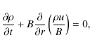
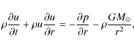
The one-fluid flow is taken to be along the radially oriented axis of a diverging flux tube, so that the bulk velocity u, (proton or electron) number density n, mass density $\rho = nm_{\rm p}$ , temperature T, thermal pressure p = 2nkT, and magnetic field Bare functions of heliocentric distance r and time t only. Wave acceleration is omitted. The mass, momentum, and energy conservation equations are then given by

$\begin{displaymath} \frac{\partial\rho}{\partial t} + B\frac{\partial}{\partial r}\left( \frac{\rho u}{B}\right) = 0, \end{displaymath}$

(1)

$\begin{displaymath} \rho\frac{\partial u}{\partial t} + \rho u\frac{\partial u}... ... = -\frac{\partial p}{\partial r} -\rho\frac{GM_\odot}{r^2}, \end{displaymath}$

(2)

$\displaystyle 3nk\left(\frac{\partial T}{\partial t} + u\frac{\partial T}{\part... ...ial r}\left[\frac{\left(F_{\rm h}+F_{\rm c} \right)}{B}\right] - n^2\Lambda(T).$

(3)

In the energy equation, the ratio of specific heats has been set to 5/3, while $F_{\rm h}$ , $F_{\rm c}$ , and $\Lambda$ respectively denote the mechanical heating flux, the conductive heating flux, and the radiative loss rate.

The magnetic field is assigned the form

$\begin{displaymath} B(r) = B_0\left(\frac{R_\odot}{r}\right)^\nu\left[\frac{1 +... ...\nu-2}}{1 + \left(R_\odot/R_{\rm ss}\right)^{\nu-2}}\right], \end{displaymath}$

(4)

where $\nu\geq 2$ and $R_{\rm ss} = 2.5$ $R_\odot$ . The field strength thus falls off as $r^{-\nu}$ for $r\lesssim 2.5$ $R_\odot$ and as r^-2 for $r\gg 2.5$ $R_\odot$ .

The mechanical heating flux $F_{\rm h}$ function is assigned different forms in the subsequent sections. Firstly, we assign it a standard phenomenological form (see, e.g., Withbroe 1988)

$\begin{displaymath} F_{\rm h} = F_{\rm p0} \left(\frac{B}{B_0}\right) \exp\left[-\frac{r-R_\odot}{H_{\rm p}}\right] \end{displaymath}$

(5)

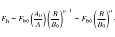
where $H_{\rm p}$ represents an arbitrary damping length and $B(r) \propto 1/A\left(r\right)$ is given by Eq. (4), $A\left(r\right)$ being the fluxtube's cross sectional area. Secondly, we assume the heating rate to be proportional to a power of B such that

$\begin{displaymath} F_{\rm h} = F_{\rm b0} \left(\frac{A_0}{A}\right)\left(\fr... ...ght)^{\mu-1} = F_{\rm b0}\left(\frac{B}{B_0}\right)^{\mu}\cdot \end{displaymath}$

(6)

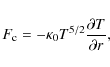
We also consider a combination of these two forms at a later time to study the effects of two separate heating sources and simulate the formation and decay of a polar plume. We assume a Spitzer-Härm conductive heating flux

$\begin{displaymath}F_{\rm c} = -\kappa_0 T^{5/2}\frac{\partial T}{\partial r}, \end{displaymath}$

(7)

where $\kappa_0 = 10^{-6}$ (in cgs units), but we modify it in two ways: a) at distances larger than 5 solar radii we limit the flux to 2/3 the Spitzer-Härm value, the width of the transition being 1 solar radius, so to prevent it from being larger than its collisionless estimation (see, e.g., Hollweg 1986,1976); b) we use an additional numerical conductive term of the form $k^{\rm num}{\partial^2 T}/{\partial r^2}$ such that $k^{\rm num}\approx\frac{c_{\rm S}\cdot\Delta z}{10^2}$ at the transition region (hereafter TR), where $c_{\rm S}$ is the sound speed and $\Delta z$ the width of the TR. This term is negligible compared to the Spitzer-Härm term everywhere except around the Transition Region, where it moderates the conductive flux and helps in keeping the mesh size not too small (see e.g, Linker et al. 2001, for comparable prescriptions). The radiative loss function is given by

$\begin{displaymath}\Lambda(T) = 10^{-22}10^{[\log_{10}(T/T_{\rm M})]^2}\chi(T) \end{displaymath}$

(8)

(based on Athay 1986), where $\chi(T)$ equals unity for T>0.02 MK and varies linearly from 0 to 1 for 0.01<T<0.02 MK. $T_{\rm M}$ equals 0.2 MK.

We employ a nonuniform grid of 640 points between the solar surface (where $\Delta r = 10^{-4}$ $R_\odot$ ) and 31.5 $R_\odot$ (where $\Delta r = 0.3$ $R_\odot$ ). Time integration is done with a Runge-Kutta scheme of order 3, while an implicit finite-difference scheme of order 6 is used for the spatial dimension, except when computing temperature gradients in the conductive term, when an explicit scheme of order 2 is applied. Numerical filtering is employed to increase the stability of the schemes (Lele 1992).

Boundary conditions are imposed by integrating the characteristic forms of Eqs. (1)-(3), as in Grappin et al. (1997). At the inner boundary, disturbances may propagate freely out of the system but not into it.

Starting with a cool (6000 K), static atmosphere, the corona and transition region are constructed as follows. During the first phase, which lasts for $\tau = R_\odot /c_{\rm s0} = 90$ min ( $c_{\rm s0}$ being the isothermal sound speed corresponding to 1 MK), the medium is heated and only $T\!\left(r\right)$ is solved for, with $P\!\left(r\right)$ being given by the equation of hydrostatic equilibrium. This preliminary phase allows considerable CPU time savings. During the second phase ( $1 < t/\tau < 40$ ), the full equations are integrated, and a supersonic wind is generated by lowering the pressure at the outer boundary using the ingoing characteristics; this artificial suction stops as soon as the flow there becomes supersonic, since thereafter no signal can propagate into the computational domain from outside. The simulations described here were performed by starting at the end of the second phase and varying the coronal parameters. We note that, even at $t/\tau = 40$ , the velocities are still decreasing with time in the transition zone; however, a steady-state equilibrium has been established near the top of this region (T = 0.5 MK), which we henceforth refer to as the ``coronal base''. Other details of the model will be discussed thoroughly in a forthcoming paper.

3 Dependence of the wind speed on the coronal parameters

For trial purposes, the coronal heating flux is first assigned the standard phenomenological form given by Eq. (5). The effect of varying the parameters $F_{\rm p0}$ , $\nu$ , and $H_{\rm p}$ is illustrated by the four steady-state wind solutions in Fig. 1. When the magnitude $F_{\rm p0}$ of the heating is raised from 4 to $8\times 10^5$ erg cm^-2 s^-1 but the other parameters are fixed, the maximum temperature $T_{\rm max}$ (attained at $R_{\rm max} = 1.88$ $R_\odot$ ) increases by 17%, while the flow speed u₁ at the outer boundary increases by 14%. The main effect, however, is to double the mass flux at the coronal base: because of the dominance of the gravitational potential energy near the solar surface, $F_{\rm p0}$ scales roughly as $\rho_0u_0 GM_\odot/R_\odot$ .

If now the magnetic falloff index $\nu$ is increased from 2 to 3 while keeping $F_{\rm p0}$ fixed at $8\times 10^5$ erg cm^-2 s^-1, the result (dashed curves in Fig. 1) is that $T_{\rm max}$ falls by 11% (mainly due to the effect of adiabatic expansion), n₀u₀ remains essentially unchanged, and u₁ decreases by 6%. This result differs from that obtained when the flux-tube divergence rate is increased but the coronal temperature is arbitrarily held fixed, in which case the mass flux at the Sun rises steeply and the asymptotic wind speed undergoes a much larger decrease (Wang & Sheeley 1991).

The dotted curves in Fig. 1 show the solution obtained when $H_{\rm p}$ is decreased from 1 to 0.5 $R_\odot$ , keeping $\nu = 3$ and $F_{\rm p0} = 8\times 10^5$ erg cm^-2 s^-1. The location of the temperature maximum moves inward as expected (from 1.73 to 1.48 $R_\odot$ ), $T_{\rm max}$ decreases by 4%, while the temperatures fall significantly in the region $r > R_{\rm max}$ . At the same time, n₀u₀ increases by 32% and u₁ drops steeply from 373 to 274 km s^-1.

$\begin{figure} \par\includegraphics[width=9cm,clip]{1183fig1.eps} \end{figure}$

Figure 1:

Four steady-state wind solutions obtained by varying the base flux density $F_{\rm p0}$ , the magnetic falloff index $\nu$ , and the damping length H in the coronal heating function $F_{\rm h}(r) = F_{\rm p0}(B/B_0)\exp[-(r-R_\odot)/H]$ . Thin solid lines: $F_{\rm p0} = 4\times 10^5$ erg cm^-2 s^-1, $\nu = 2$ , H = 1 $R_\odot$ . Thick solid lines: $F_{\rm p0} = 8\times 10^5$ erg cm^-2 s^-1, $\nu = 2$ , H = 1 $R_\odot$ . Dashed lines: $F_{\rm p0} = 8\times 10^5$ erg cm^-2 s^-1, $\nu = 3$ , H = 1 $R_\odot$ . Dotted lines: $F_{\rm p0} = 8\times 10^5$ erg cm^-2 s^-1, $\nu = 3$ , H = 0.5 $R_\odot$ . Top panel shows $F_{\rm h}(r)/(10^5$ erg cm^-2 s^-1), u(r)/(100 km s^-1), and T(r)/(1 MK); bottom panel shows $n(r)\ [$ cm^-3] and $n(r)u(r)\ [10^8$ cm^-2 s^-1].

Open with DEXTER

$\begin{figure} \par\includegraphics[width=9cm,clip]{1183fig2.eps} \end{figure}$	Figure 2: Three steady-state wind solutions obtained by varying the magnetic falloff index in the coronal heating function $F_{\rm h}(r) = 8\times 10^5$ erg cm^-2 s^-1 (B/B₀)^3/2. Thin solid lines: $\nu = 2$ . Thick solid lines: $\nu = 3$ . Dashed lines: $\nu = 4$ . Dotted lines: $\nu = 5$ .
Open with DEXTER

These calculations suggest that the parameter to which the asymptotic wind speed is most sensitive is the location of the coronal heating. In particular, depositing the bulk of the energy near the coronal base results in lower wind speeds and higher mass fluxes, whereas depositing it near the sonic point produces higher wind speeds and lower mass fluxes (see Leer & Holzer 1980). Here, the damping length $H_{\rm p}$ has been treated as an arbitrary parameter. However, if the source of the heating is magnetic in nature, its spatial distribution might be expected to depend on $B\left(r\right)$ , with the damping length being smaller, the more rapidly the field strength falls off with height (for example, $H/R_\odot\propto \nu^{-\alpha}$ , where $\alpha > 0$ ). Indeed, Cranmer et al. (2007) have developed a self-consistent model for coronal heating and solar wind acceleration, in which the wind speed and mass flux are determined by the radial gradient of the Alfvén speed. In this model, the coronal hole is heated by the damping of Alfvén waves via a turbulent cascade; the turbulent heating rate is inversely proportional to the transverse correlation length $L_\perp$ , which in turn varies as B^-1/2 (cf. Hollweg 1986).

To demonstrate that a coronal mechanical heating flux that depends mainly on the local magnetic field strength will necessarily lead to an inverse relationship between wind speed and expansion factor, let us use the heating flux as given by Eq. (6) where, for illustrative purposes, we take $\mu = 3/2$ . Figure 2 shows the steady-state wind solutions obtained by setting $\nu$ equal to 2, 3, 4 and 5. As the magnetic falloff rate increases, the location of the temperature maximum moves inward, its peak value decreases, n₀u₀increases, the outer region $r > R_{\rm max}$ becomes cooler, and the flow velocity at the outer boundary drops. Similar results are obtained for any $\mu > 1$ .

$\begin{figure} \par\includegraphics[width=9cm,clip]{1183fig3.eps} \end{figure}$	Figure 3: Time evolution of the $\nu = 2$ wind solution in Fig. 2, after $F_{\rm b0}$ is suddenly decreased from 8 to $1\times 10^5$ erg cm^-2 s^-1. The radial profiles of u, T, and n are plotted at $t/\tau = 0$ (thick continuous lines), 1, 2, 3, 4, 5, 7, 10, 15, 25 (dashed lines) and 40 (thin continuous line) where $\tau = R_\odot /c_{\rm s0} = 90$ min.
Open with DEXTER

$\begin{figure} \par\includegraphics[width=9cm,clip]{1183fig4} \end{figure}$

Figure 4:

Here, the magnetic falloff index $\nu$ is suddenly increased from 2 to 10 while keeping $F_{\rm b0}$ fixed at $8\times 10^5$ erg cm^-2 s^-1. The radial profiles of u, T, and n are shown at $t/\tau = 0$ (thick continuous lines), 1, 2, 3, 4, 5, 7, 10, 15, 25 (dashed lines) and 40 (thin continuous line). Strong inflows are generated below the sonic point (represented by the diamond marks over each u profile), which moves progressively outwards.

Open with DEXTER

4 Generating coronal inflows

During times of high solar activity, white-light coronagraph observations often show swarms of small-scale features moving sunward in the region 2 $R_\odot\lesssim r\lesssim 5$ $R_\odot$ (Sheeley & Wang 2002). These inflow events are concentrated around the heliospheric current/plasma sheet. They characteristically start as small density enhancements that accelerate from rest and leave a narrow, dark trail in their wake, subsequently decelerating as they approach the inner edge of the coronagraph field of view. Although some of these events are clearly CME-associated, the majority do not occur in the immediate aftermath of CMEs and appear to represent the closing-down of magnetic flux at coronal hole boundaries.

In the simulation shown in Fig. 3, we have started with the $\nu = 2$ wind solution of Fig. 2 and then instantaneously reduced $F_{\rm b0}$ from 8 to $1\times 10^5$ erg cm^-2 s^-1(see Eq. (6)). The radial profiles of T, u, and n are plotted at a succession of times $t/\tau = 0$ , 2, 4, 10, 20 and 40 where $\tau = R_\odot /c_{\rm s0} = 90$ min and t = 0 is here defined as the moment when the heating is turned down. Although the temperatures almost immediately drop toward their new equilibrium values, the flow velocities and densities require on the order of a global sound-crossing time ( ${\sim }30$ $R_\odot/c_{\rm s0}$ ) to adjust to the greatly reduced heating rate. In the expanding subsonic regime, the flow separates into inward- and outward-moving components, and the density falls. Outflow from the Sun is reestablished after $t\sim 10\tau$ , and the system reaches a steady state with reduced velocities and densities by $t\sim 20\tau$ . While this simulation produces modest inflows near the Sun, it is unclear how a large decrease in $F_{\rm b0}$ might be effected in reality.

The closing-down of magnetic flux requires that open field lines of opposite polarity be brought together and reconnected with each other. Since the local field strength is small in the vicinity of the polarity reversal, any flux tube that undergoes this merging process must diverge rapidly with radial distance, and the outward extension of this flux tube must experience a large reduction in its heating rate according to Eq. (6). Instead of decreasing the amplitude of the heating function as in the simulation of Fig. 3, let us now keep $F_{\rm b0}$ fixed at $8\times 10^5$ erg cm^-2 s^-1 but increase the magnetic falloff index $\nu$ from 2 to 10. As shown in Fig. 4, the velocity profile again collapses and inflows are generated below the sonic point, which moves progressively outward. In this case, because the heating remains strong near the solar surface, the density increases with time at low heights, where hydrostatic equilibrium is approached. Above $r\sim 3$ $R_\odot$ , however, the inward velocities continue to grow to amplitudes of nearly 100 km s^-1 and n(r) falls sharply. The squeezing-out of plasma from the flux tubes in this region should facilitate the merging and reconnection process.

$\begin{figure} \par\includegraphics[width=9cm,clip]{1183fig5.eps} \end{figure}$

Figure 5:

Effect of an additional heating term near the coronal base, of the form $F_{\rm p0}(B/B_0)\exp[-(r-R_\odot)/H_{\rm p}]$ . Solid curves: steady-state ``plume'' solution with $F_{\rm p0} = 4\times 10^5$ erg cm^-2 s^-1 and $H_{\rm p0} = 0.05$ $R_\odot$ . Dashed curves: steady-state ``interplume'' solution with $F_{\rm p0} = 0$ . In both cases, the global heating term is given by $F_{\rm b0}(B/B_0)^{3/2}$ , with $F_{\rm b0} = 4\times 10^5$ erg cm^-2 s^-1 and $\nu = 2$ .

Open with DEXTER

$\begin{figure} \par\includegraphics[width=9cm,clip]{1183fig6.eps} \end{figure}$	Figure 6: Radial profiles of the heating function, conductive heating flux, and enthalpy flux for the plume and interplume solutions.
Open with DEXTER

$\begin{figure} \par\includegraphics[width=9cm,clip]{1183fig7.eps} \end{figure}$

Figure 7:

Formation of a plume. With the initial state being given by the interplume solution ( $F_{\rm p0} = 0$ , $F_{\rm b0} = 4\times 10^5$ erg cm^-2 s^-1, $\nu = 2$ ), $F_{\rm p0}$ is suddenly increased to $4\times 10^5$ erg cm^-2 s^-1. The radial profiles of u, T, and n are shown at $t/\tau = 0$ (thick continuous lines), 1, 2, 3, 4, 5, 7, 10, 15, 25 (dashed lines) and 40 (thin continuous line)

Open with DEXTER

$\begin{figure} \par\includegraphics[width=9cm,clip]{1183fig8.eps} \end{figure}$	Figure 8: Decay of a plume. With the initial state now being given by the plume solution ( $F_{\rm p0} = 4\times 10^5$ erg cm^-2 s^-1, $H_{\rm p} = 0.05$ $R_\odot$ ), $F_{\rm p0}$ is suddenly set to 0. The radial profiles of u, T, and n are plotted at $t/\tau = 0$ (thick continuous lines), 1, 2, 3, 4, 5, 7, 10, 15, 25 (dashed lines) and 40 (thin continuous line).
Open with DEXTER

$\begin{figure} \par\includegraphics[width=9cm,clip]{1183fig9} \end{figure}$	Figure 9: Peak inflow amplitude $u_{\rm inflow}$ as a function of the heating timescale $\delta t/\tau$ , where $\tau = 90$ min, for the variation of the magnetic falloff index $\nu$ from 2 to 10, as in Fig. 4. The position of the inflow peak - about $r=3.5\ R_\odot$ - doesn't depend on the value of $\delta t$ .
Open with DEXTER

5 Formation of a polar plume

Coronal plumes are raylike features aligned along open field lines and characterized by densities $\sim$ 2-5 times higher than the surrounding interplume regions of the coronal hole. As shown in Wang (1994a), the enhanced densities in plumes require the presence of a strong heating source near their bases. Indeed, plumes are found to overlie EUV bright points, and these small bipoles appear to be undergoing interchange reconnection with the unipolar flux concentrations inside coronal holes.

The effect of two separate heating sources, one spread over a distance on the order of a solar radius, the other concentrated at the base of the flux tube, is illustrated by the steady-state wind solution in Fig. 5. Here the total heating function is taken to be of the form

$\begin{displaymath}F_{\rm plume} = F_{\rm b0}\left(B/B_0\right)^{3/2} + F_{\rm... .../B_0\right)\exp\left[-\left(r-R_\odot\right)/H_{\rm p}\right], \end{displaymath}$

(9)

with $F_{\rm b0} = 4\times 10^5$ erg cm^-2 s^-1 and $\nu = 2$ . The ``interplume'' solution, for which $F_{\rm p0} = 0$ , is indicated by the dotted curves. The plume solution (solid curves) has $F_{\rm p0} = F_{\rm b0} = 4\times 10^5$ erg cm^-2 s^-1 and $H_{\rm p} = 0.05$ $R_\odot$ . The extra base heating causes T(r) to increase near the coronal base but to decrease at greater heights; at the same time, u(r) falls and n(r) rises everywhere. The factor of $\sim$ 4 increase in the density is accompanied by a sharp rise in the conductive heating flux $F_{\rm c} = -\kappa_0 T^{5/2}{\rm d}T/{\rm d}r$ conducted downward into the transition region and by a large increase in the outward enthalpy flux $F_{\rm enthpy} = 5pu/2$ (Fig. 6).

Figure 7 shows how the plume forms as the base heating rate $F_{\rm p0}$ is suddenly raised from 0 to $4\times 10^5$ erg cm^-2 s^-1. The velocities increase during the first several hours, but subsequently fall below the initial (interplume) values as the densities continue to rise and the plasma above the coronal base cools. The reverse process, in which the base heating is suddenly switched off, is shown in Fig. 8. The velocities initially decrease, even becoming slightly negative ( $u_0\sim -1$ km s^-1) near the coronal base; the equilibrium profile, in which the speeds are everywhere higher than the plume values, is attained only after $\sim$ 1 day. We note that it takes as long as $\sim$ 5 h. for the densities to drop by a factor of two, a result that is consistent with the observed tendency for EUV ``plume haze'' to linger well after the underlying bright point has faded.

6 Heating timescale and inflow amplitudes

The inflows observed in Figs. 3, 4 and 8, as well as the ``jet'' shown in Fig. 7, are transient structures which propagate away from a well defined region where the volumetric heating rate changes. These sound wavefronts are the response to the pressure variations which correspond to the volumetric heating rate changes within that region. Take for example the case described in Fig. 4, where the magnetic falloff index $\nu$ was increased abruptly from 2 to 10, which translates into a decrease in the heating rate in the region between $r=1\ R_\odot$ and $r=R_{\rm ss}=2.5\ R_\odot$ (for $r>R_{\rm ss}$ , $B\propto r^{-2}$ at all times; see Eq. (4) for the definition of the magnetic field and Eq. (6) for the heating flux used). We observe the evolution of a negative velocity perturbation $\delta u_{\rm inflow}$ which is superposed on the background wind flow. The wind slows down as the wavefront passes through. The resulting total velocity can then be negative, especially in the lower corona (below $3{-}5\ R_\odot$ ) where the solar wind speed is still low. This produces a transient accretion event. Figure 9 shows the maximum inflow amplitude as a function of the transition time $\delta t$ for the variation of the magnetic falloff index $\nu$ . The transient inflow amplitude decreases as $\delta t$ increases, i.e, as the heating variation becomes less and less abrupt. The inflow peak velocity only drops down to zero for $\delta t/\tau \approx 50$ , which is much longer than the sound-crossing time $\tau_{\rm cs}/\tau = 0.96$ of the region where the heating rate changes. The position of the inflow peak velocity ( ${\sim} 3.5\ R_\odot$ ), its spatial width ( ${\sim} 2\ R_\odot$ ) and the final stationary state do not depend on $\delta t$ .

7 Conclusions

We have used a one-dimensional hydrodynamic code to demonstrate how variations in the coronal heating function can produce a wide variety of solar wind flows. In particular, we find that:

1.: The observed inverse correlation between wind speed and expansion factor can be explained if the heating rate depends mainly on the local magnetic field strength. In that case, most of the heating in a rapidly diverging field will occur well inside the sonic point, resulting in a large mass flux at the coronal base and a low flow speed far from the Sun.
2.: Strong inflows can be generated in the subsonic region by decreasing the local heating rate. Such a decrease might occur during the closing-down of flux, when opposite-polarity field lines merge at a neutral sheet. The evacuation of the flux tubes would further accelerate the merging and reconnection process.
3.: Densities comparable to those observed in polar plumes can be obtained by depositing a large amount of energy just above the coronal base. When this extra heating is switched on, the temperature rises locally but falls at greater heights, the densities progressively increase all along the flux tube, while the velocities initially increase but subsequently decrease below their initial values. The process is reversed when the base heating is switched off. In either case, a steady-state equilibrium is reached only after $\sim$ 1 day, which may explain why coronal plumes appear to evolve more slowly than their underlying EUV bright points.

Our simulations suggest that it is unnecessary to invoke sources outside of coronal holes for the bulk of the slow solar wind. However, we note that the material within the heliospheric plasma sheet most likely originates from closed helmet-streamer loops, being tranferred to the open field region by interchange reconnection (Wang et al. 1998; Crooker et al. 2004).

Our future objective is to extend the numerical code to two and three dimensions, while solving the full MHD equations with consistent dissipative terms. It may then be possible to provide a more physical description of the coronal heating process, generalizing the one-dimensional model of Suzuki & Inutsuka (2006), in which Alfvén waves drive compressional waves that dissipate in the corona.

Acknowledgements

This work was supported by CNRS, NASA, and the Office of Naval Research.

References

Arge, C. N., & Pizzo, V. J. 2000, J. Geophys. Res., 105, 10465 In the text
Athay, R. G. 1986, ApJ, 308, 975 In the text
Cranmer, S. R., van Ballegooijen, A. A., & Edgar, R. J. 2007, ApJS, 171, 520 In the text
Crooker, N. U., Huang, C.-L., Lamassa, S. M., et al. 2004, J. Geophys. Res. (Space Physics), 109, 3107 In the text
Grappin, R., Cavillier, E., & Velli, M. 1997, A&A, 322, 659 In the text
Hammer, R. 1982, ApJ, 259, 767 In the text
Hollweg, J. V. 1976, J. Geophys. Res., 81, 1649 In the text
Hollweg, J. V. 1986, J. Geophys. Res., 91, 4111 In the text
Leer, E., & Holzer, T. E. 1980, J. Geophys. Res., 85, 4681 In the text
Lele, S. K. 1992, J. Comput. Phys., 103, 16 In the text
Levine, R. H., Altschuler, M. D., & Harvey, J. W. 1977, J. Geophys. Res., 82, 1061 In the text
Linker, J. A., Lionello, R., Mikic, Z., & Amari, T. 2001, J. Geophys. Res., 106, 25165 In the text
Poduval, B., & Zhao, X. P. 2004, J. Geophys. Res. (Space Physics), 109, 8102 In the text
Sandbaek, O., Leer, E., & Hansteen, V. H. 1994, ApJ, 436, 390 In the text
Sheeley, Jr., N. R., & Wang, Y.-M. 2002, ApJ, 579, 874 In the text
Suzuki, T. K., & Inutsuka, S.-i. 2006, J. Geophys. Res. (Space Physics), 111, 6101 In the text
Wang, Y.-M. 1993, ApJ, 410, L123 In the text
Wang, Y.-M. 1994a, ApJ, 435, L153 In the text
Wang, Y.-M. 1994b, ApJ, 437, L67 In the text
Wang, Y.-M., & Sheeley, Jr., N. R. 1990, ApJ, 355, 726 In the text
Wang, Y.-M., & Sheeley, Jr., N. R. 1991, ApJ, 372, L45 In the text
Wang, Y.-M., Sheeley, Jr., N. R., Walters, J. H., et al. 1998, ApJ, 498, L165 In the text
Whang, Y. C., Wang, Y.-M., Sheeley, N. R., & Burlaga, L. F. 2005, J. Geophys. Res. (Space Physics), 110, 3103 In the text
Withbroe, G. L. 1988, ApJ, 325, 442 In the text
Zurbuchen, T. H. 2007, ARA&A, 45, 297 In the text

All Figures

$\begin{figure} \par\includegraphics[width=9cm,clip]{1183fig1.eps} \end{figure}$	Figure 1: Four steady-state wind solutions obtained by varying the base flux density $F_{\rm p0}$ , the magnetic falloff index $\nu$ , and the damping length H in the coronal heating function $F_{\rm h}(r) = F_{\rm p0}(B/B_0)\exp[-(r-R_\odot)/H]$ . Thin solid lines: $F_{\rm p0} = 4\times 10^5$ erg cm^-2 s^-1, $\nu = 2$ , H = 1 $R_\odot$ . Thick solid lines: $F_{\rm p0} = 8\times 10^5$ erg cm^-2 s^-1, $\nu = 2$ , H = 1 $R_\odot$ . Dashed lines: $F_{\rm p0} = 8\times 10^5$ erg cm^-2 s^-1, $\nu = 3$ , H = 1 $R_\odot$ . Dotted lines: $F_{\rm p0} = 8\times 10^5$ erg cm^-2 s^-1, $\nu = 3$ , H = 0.5 $R_\odot$ . Top panel shows $F_{\rm h}(r)/(10^5$ erg cm^-2 s^-1), u(r)/(100 km s^-1), and T(r)/(1 MK); bottom panel shows $n(r)\ [$ cm^-3] and $n(r)u(r)\ [10^8$ cm^-2 s^-1].
Open with DEXTER
In the text

$\begin{figure} \par\includegraphics[width=9cm,clip]{1183fig2.eps} \end{figure}$	Figure 2: Three steady-state wind solutions obtained by varying the magnetic falloff index in the coronal heating function $F_{\rm h}(r) = 8\times 10^5$ erg cm^-2 s^-1 (B/B₀)^3/2. Thin solid lines: $\nu = 2$ . Thick solid lines: $\nu = 3$ . Dashed lines: $\nu = 4$ . Dotted lines: $\nu = 5$ .
Open with DEXTER
In the text

$\begin{figure} \par\includegraphics[width=9cm,clip]{1183fig3.eps} \end{figure}$	Figure 3: Time evolution of the $\nu = 2$ wind solution in Fig. 2, after $F_{\rm b0}$ is suddenly decreased from 8 to $1\times 10^5$ erg cm^-2 s^-1. The radial profiles of u, T, and n are plotted at $t/\tau = 0$ (thick continuous lines), 1, 2, 3, 4, 5, 7, 10, 15, 25 (dashed lines) and 40 (thin continuous line) where $\tau = R_\odot /c_{\rm s0} = 90$ min.
Open with DEXTER
In the text

$\begin{figure} \par\includegraphics[width=9cm,clip]{1183fig4} \end{figure}$	Figure 4: Here, the magnetic falloff index $\nu$ is suddenly increased from 2 to 10 while keeping $F_{\rm b0}$ fixed at $8\times 10^5$ erg cm^-2 s^-1. The radial profiles of u, T, and n are shown at $t/\tau = 0$ (thick continuous lines), 1, 2, 3, 4, 5, 7, 10, 15, 25 (dashed lines) and 40 (thin continuous line). Strong inflows are generated below the sonic point (represented by the diamond marks over each u profile), which moves progressively outwards.
Open with DEXTER
In the text

$\begin{figure} \par\includegraphics[width=9cm,clip]{1183fig5.eps} \end{figure}$	Figure 5: Effect of an additional heating term near the coronal base, of the form $F_{\rm p0}(B/B_0)\exp[-(r-R_\odot)/H_{\rm p}]$ . Solid curves: steady-state ``plume'' solution with $F_{\rm p0} = 4\times 10^5$ erg cm^-2 s^-1 and $H_{\rm p0} = 0.05$ $R_\odot$ . Dashed curves: steady-state ``interplume'' solution with $F_{\rm p0} = 0$ . In both cases, the global heating term is given by $F_{\rm b0}(B/B_0)^{3/2}$ , with $F_{\rm b0} = 4\times 10^5$ erg cm^-2 s^-1 and $\nu = 2$ .
Open with DEXTER
In the text

$\begin{figure} \par\includegraphics[width=9cm,clip]{1183fig6.eps} \end{figure}$	Figure 6: Radial profiles of the heating function, conductive heating flux, and enthalpy flux for the plume and interplume solutions.
Open with DEXTER
In the text

$\begin{figure} \par\includegraphics[width=9cm,clip]{1183fig7.eps} \end{figure}$	Figure 7: Formation of a plume. With the initial state being given by the interplume solution ( $F_{\rm p0} = 0$ , $F_{\rm b0} = 4\times 10^5$ erg cm^-2 s^-1, $\nu = 2$ ), $F_{\rm p0}$ is suddenly increased to $4\times 10^5$ erg cm^-2 s^-1. The radial profiles of u, T, and n are shown at $t/\tau = 0$ (thick continuous lines), 1, 2, 3, 4, 5, 7, 10, 15, 25 (dashed lines) and 40 (thin continuous line)
Open with DEXTER
In the text

$\begin{figure} \par\includegraphics[width=9cm,clip]{1183fig8.eps} \end{figure}$	Figure 8: Decay of a plume. With the initial state now being given by the plume solution ( $F_{\rm p0} = 4\times 10^5$ erg cm^-2 s^-1, $H_{\rm p} = 0.05$ $R_\odot$ ), $F_{\rm p0}$ is suddenly set to 0. The radial profiles of u, T, and n are plotted at $t/\tau = 0$ (thick continuous lines), 1, 2, 3, 4, 5, 7, 10, 15, 25 (dashed lines) and 40 (thin continuous line).
Open with DEXTER
In the text

$\begin{figure} \par\includegraphics[width=9cm,clip]{1183fig9} \end{figure}$	Figure 9: Peak inflow amplitude $u_{\rm inflow}$ as a function of the heating timescale $\delta t/\tau$ , where $\tau = 90$ min, for the variation of the magnetic falloff index $\nu$ from 2 to 10, as in Fig. 4. The position of the inflow peak - about $r=3.5\ R_\odot$ - doesn't depend on the value of $\delta t$ .
Open with DEXTER
In the text

Current usage metrics show cumulative count of Article Views (full-text article views including HTML views, PDF and ePub downloads, according to the available data) and Abstracts Views on Vision4Press platform.

Data correspond to usage on the plateform after 2015. The current usage metrics is available 48-96 hours after online publication and is updated daily on week days.

Initial download of the metrics may take a while.