| Issue |
A&A
Volume 497, Number 1, April I 2009
|
|
|---|---|---|
| Page(s) | 265 - 272 | |
| Section | The Sun | |
| DOI | https://doi.org/10.1051/0004-6361/200811481 | |
| Published online | 24 February 2009 | |
The influence of longitudinal density variation in coronal loops on the eigenfunctions of kink-oscillation overtones
J. Andries1,2,![]() - I. Arregui3 - M. Goossens1
- I. Arregui3 - M. Goossens1
1 - Centrum voor Plasma Astrofysica and Leuven Mathematical Modelling and Computational Science Centre, KULeuven, Celestijnenlaan 200B, 3001 Leuven, Belgium
2 -
Centre for Stellar and Planetary Astrophysics, Monash University, 3800 Victoria, Australia
3 -
Departament de Física, Universitat de les Illes Balears, 07122 Palma de Mallorca, Spain
Received 8 December 2008 / Accepted 24 January 2009
Abstract
Context. As coronal loops are spatially at least partially resolved in the longitudinal direction, attempts have been made to use the longitudinal profiles of the oscillation amplitudes as a seismological tool.
Aims. We aim to derive simple formulae to assess which oscillation modes and which quantities of the oscillation (displacement or compression) are most prone to modifications induced by stratification of the equilibrium density along the loop. We furthermore clarify and quantify that the potential of such a method could be enhanced if observational profiles of the compression in the oscillations could be determined.
Methods. By means of a linear expansion in the longitudinal stratification along with the ``thin tube'' approximation, the modifications to the eigenfunctions are calculated analytically. The results are validated by direct numerical computations.
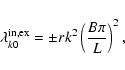
Results. Higher axial overtones are found to be more affected by equilibrium stratification and hence would provide a much better tool if observed. For the k-1th overtone the compression is found to be around
(k+2)2/k2 times more sensitive to longitudinal density variation than the displacement. While the linear formulae do give a good indication of the strength of the effects of longitudinal density stratification, the numerical computations indicate that the corrections to the approximate analytical results are significant and cannot be neglected under the expected coronal conditions.
Key words: magnethohydrodynamics (MHD) - waves - Sun: corona - Sun: oscillations - Sun: magnetic fields
1 Introduction
The clear detection of flare generated coronal loop oscillations by the Transition Region and Coronal Explorer has initiated the field of coronal loop seismology. An interpretation of the oscillations in terms of the fundamental kink oscillation of a coronal flux tube (as treated by Edwin & Roberts 1983) enabled investigators to deduce a rough estimate for the coronal magnetic field strength from the observed periodicity (Nakariakov & Ofman 2001; Nakariakov 2000). Ruderman & Roberts (2002) subsequently extended the basic model to include smooth transversal density variations which give rise to a continuous spectrum and associated continuum damping, also known as Alfvén resonant absorption. Within that framework the additional model parameter that quantifies the transversal density inhomogeneity length scale can directly be related to the damping time of the oscillations (Goossens et al. 2002). In recent studies by Arregui et al. (2007) and Goossens et al. (2008) the third remaining parameter of the density contrast between the loop and the surrounding plasma (which was assigned an ad hoc value in all previous studies) was taken into account consistently.The simultaneous detection of axial overtones of a coronal loop kink-mode oscillation by Verwichte et al. (2004) has triggered an increased interest for theoreticians to refine the theoretical modelling of transverse coronal loop oscillations, and has greatly advanced coronal seismology (for reviews see Roberts 2008; Nakariakov & Verwichte 2005). With regard to the potential of coronal seismology, the discovery of harmonic coronal loop oscillations has raised awareness on two important issues.
Firstly, the simultaneous detection of several oscillation frequencies is an important advance in the development of any seismological endeavour. It allows us to add complexity to the proposed theoretical models and infer values for the additional parameters without detailed spatial resolution of the oscillations. In a coronal context, this was first illustrated by Andries et al. (2005a) by means of the computations of eigenfrequencies and eigenmodes in coronal loop models with longitudinal density stratification (Andries et al. 2005b) (using a method similar to that of Díaz et al. 2002,2004). The deviation of the ratio of the fundamental period to the successive overtones from 1/2, 1/3, etc. was related to, and hence used as a measure for, the density scale height. McEwan et al. (2006) investigated alternative explanations for the anomalous period ratio but concluded that it is most probably due to longitudinal density stratification (or magnetic field variation, which had not been assessed at that time). Meanwhile much more theoretical as well as observational work has been done along those lines (Díaz et al. 2006; De Moortel & Brady 2007; Van Doorsselaere et al. 2007; McEwan et al. 2008; Dymova & Ruderman 2006a; Donnelly et al. 2006; Dymova & Ruderman 2006b; Díaz et al. 2007). Verth & Erdélyi (2008) and Ruderman et al. (2008) included the variation of the magnetic field along the loop into the calculations. They concluded that it has an effect opposite to that of the density variation and may alter the seismologically inferred density scale heights considerably. By using observational estimates of the magnetic field expansion Verth et al. (2008) performed a refined seismological analysis of the density scale height by means of the period ratio.
Secondly, since the identification of the first overtone in the observations was not only made because of its frequency close to twice that of the fundamental, but also by observational evidence that the amplitude of that mode had maxima halfway down the loop legs and a node at the loop top, this made it clear that at least in the axial direction we are able at present to partly resolve the spatial structure of the oscillations. It was strongly emphasised by Erdélyi & Verth (2007) and Verth et al. (2007) that the longitudinal spatial resolution could possibly allow for the estimation of loop model parameters based on the deviations in the eigenfunctions rather than the eigenfrequencies. The effect of longitudinal density stratification on the transversal displacement amplitude was however found to be not particularly strong for the fundamental oscillation (Erdélyi & Verth 2007; Safari et al. 2007), and due to several uncertainties in the observations (projection effects, localisation of the loop footpoints), probably not detectable at present with reasonable confidence. For the first overtone however it was found that the shift of the antinodes towards the footpoints is much more pronounced and could possibly be detectable. Progress in these detections could possibly be sought in advanced edge tracking detection methods as used by Jess et al. (2008).
The present paper aims at contributing to this second point.
We derive simple algebraic expressions that quantify how much the eigenfunctions are altered by the presence of a longitudinal density variation. In order to arrive at analytical expressions, we assume a relatively weak density structuring which is identical inside and outside the loop. The expressions are derived generally, valid for any harmonic, and both for the displacement and the compression. The derivation starts from a tube of arbitrary thickness but eventually specializes to a ``thin tube'' to obtain concise formulae. A similar formula (for the displacement only) was derived by Safari et al. (2007) starting directly from the ``thin tube'' formula by Dymova & Ruderman (2005). They used it to validate the results about the modifications to the displacement profiles of the fundamental and its first harmonic by Erdélyi & Verth (2007) and Verth et al. (2007). However, the formulae enable us to assess whether higher harmonics, if they could possibly be detected in the future, would have even higher potential for spatial seismology. The answer is clearly affirmative. However, it is debatable whether the shift of the antinodes is in general a good observational signature of the modifications to the eigenfunctions.
Secondly, the derivations also address a conclusion which was already made by Andries et al. (2005b) but which has not received much attention so far. From the numerical computations it was concluded that the influence on the eigenfunctions seems to be much more pronounced in the total pressure perturbation than in the transversal displacement although a quantitative analysis was not performed. Observationally however, it is the displacement which is measured. Being nearly incompressible, it is clear that kink modes are most easily detected as transverse displacements and measuring the compression in the observations is probably not easy to achieve. We want to argue however that from a theoretical perspective the potential for revealing information on the longitudinal structure by means of analysis of the spatial eigenfunctions is much greater if the compression or the density variation could be measured.
In Sect. 2 the approximate formulae for the modifications of the eigenmodes are derived analytically. Based on these formulae it is discussed in Sect. 3 how the different harmonics are influenced. In Sect. 4 the validity of these formulae is checked numerically.
2 Model and analysis
2.1 Model and setup
The loop model is exactly as in Andries et al. (2005b). The coronal loop is viewed as a straight cylindrical flux tube where the magnetic field is constant but the density varies both in the radial (hence characterising the tube as a density enhancement) and longitudinal direction. The slow waves are removed from the analysis as ![]() is an appropriate approximation in the lower corona. As before the observed oscillations are modelled as linear oscillations because the observed velocities are small compared to the local Alfvén speed. Within the linear treatment this is equivalent to the observation that the displacement is small compared to the length of the loop. However, in a different context, the nonlinear coupling between different azimuthal components has been related to the ratio between the displacement and the tube radius (Ruderman 1992). At present it is not clear how important this effect of non-linear coupling of azimuthal wave numbers is for standing kink oscillations.
is an appropriate approximation in the lower corona. As before the observed oscillations are modelled as linear oscillations because the observed velocities are small compared to the local Alfvén speed. Within the linear treatment this is equivalent to the observation that the displacement is small compared to the length of the loop. However, in a different context, the nonlinear coupling between different azimuthal components has been related to the ratio between the displacement and the tube radius (Ruderman 1992). At present it is not clear how important this effect of non-linear coupling of azimuthal wave numbers is for standing kink oscillations.
In a cylindrical reference frame where the equilibrium quantities are independent of ![]() and of time, the perturbed quantities can be set proportional to
and of time, the perturbed quantities can be set proportional to
![]() and
and
![]() because no coupling between different Fourier modes can occur. Here
because no coupling between different Fourier modes can occur. Here ![]() is the circular frequency and m (an integer) is the azimuthal wave number. As we are interested in oscillations that displace the axis of the loop and also the loop as a whole, we need to take m=1. This is the only value of the azimuthal wave number for which the loop is displaced. For a
loop that is uniform in the longitudinal direction the longitudinal variation of the kink oscillation can be described by one axial wave number kz with the axial behaviour proportional to
is the circular frequency and m (an integer) is the azimuthal wave number. As we are interested in oscillations that displace the axis of the loop and also the loop as a whole, we need to take m=1. This is the only value of the azimuthal wave number for which the loop is displaced. For a
loop that is uniform in the longitudinal direction the longitudinal variation of the kink oscillation can be described by one axial wave number kz with the axial behaviour proportional to
![]() .
For a loop of length L,
.
For a loop of length L,
![]() ,
n is a positive integer. n=1 corresponds to the fundamental axial mode;
,
n is a positive integer. n=1 corresponds to the fundamental axial mode; ![]() correspond to the axial overtones. A consequence of longitudinal stratification is that a given mode cannot be described by one axial wave number but now instead an infinite sine series is required. Unless the longitudinal stratification is very strong, one term in this infinite series is dominant so that we can still speak about the fundamental axial mode etc. When we speak about the kth mode in what follows, this is meant with respect to the axial ordering as we just discussed. The radial part of the spatial solutions of the modes does not follow a harmonic variation. However, the modes can be distinguished by the number of nodes in the radial part of their spatial solution. The kink oscillations invoked to explain the observed transverse oscillations in coronal loops have no nodes in the radial part of their spatial solution. They are fundamental radial kink oscillations.
correspond to the axial overtones. A consequence of longitudinal stratification is that a given mode cannot be described by one axial wave number but now instead an infinite sine series is required. Unless the longitudinal stratification is very strong, one term in this infinite series is dominant so that we can still speak about the fundamental axial mode etc. When we speak about the kth mode in what follows, this is meant with respect to the axial ordering as we just discussed. The radial part of the spatial solutions of the modes does not follow a harmonic variation. However, the modes can be distinguished by the number of nodes in the radial part of their spatial solution. The kink oscillations invoked to explain the observed transverse oscillations in coronal loops have no nodes in the radial part of their spatial solution. They are fundamental radial kink oscillations.
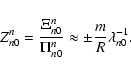
Solutions to the linearised expressions can be obtained analytically in the internal and external regions where the density does not vary with radial
position r. We follow the notation as introduced by Andries et al. (2005b), where the Eulerian pressure perturbation and the radial component of the Lagrangian displacement, both evaluated at the discontinuous boundary, are expressed as a sine series expansion (with L the loop length):
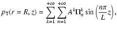 |
(1) | ||
 |
(2) |
As at the boundary surface r=R both ![]() and
and ![]() have to be continuous (in the radial direction) the dispersion relation is obtained as the determinant of the resulting infinite set of matching conditions. Without stratification
have to be continuous (in the radial direction) the dispersion relation is obtained as the determinant of the resulting infinite set of matching conditions. Without stratification ![]() and
and ![]() are zero whenever
are zero whenever ![]() ,
yielding a block diagonal system with a
,
yielding a block diagonal system with a ![]() block for each Fourier mode.
block for each Fourier mode.
The equilibrium density is expressed as a constant (in the z direction) plus a sine series expansion:
![\begin{displaymath}\rho(r,z)=\rho_0(r)\left [1+\sum_{n=1}^{+\infty}\alpha_n(r)\sin\left(\frac{n\pi}{L}z\right)\right ].
\end{displaymath}](/articles/aa/full_html/2009/13/aa11481-08/img29.gif)
In Andries et al. (2005b) we have analysed in detail how the dispersion relation can be expanded linearly in
2.2 Analysis
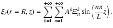
Consider the ratios of the jth term and the kth term in the sine series expansion (denoted as RPjk and RXjk for pressure and displacement) of the kth eigenmode. To first order in| |
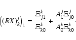
= | 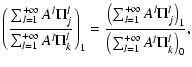 |
(4) |
| = |  |
(5) | |
| = | (6) | ||
| = |  |
(7) |
and likewise for the displacement:
 |
(8) |
The expressions for


Therefore:
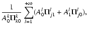
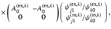
The corrections to the Alfvén eigenmodes have been calculated by Andries et al. (2005b), so what remains to be computed are the corrections Aj1 to the solution vectors. From the dispersion Eq. (6) in Andries et al. (2005b) expanded up to first order we get for fixed k and arbitrary j:
 |
(13) |
Thus formally:
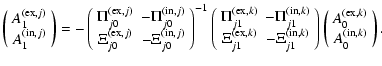 |
(14) |
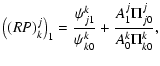
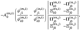
Using (9) and (10) we obtain:
 |
= |  |
|
 |
(15) |
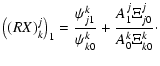
We can then further rewrite the last part and apply the zeroth order dispersion relation to find:
| |
= | |
|
 |
(16) | ||
| = | |
||
 |
(17) | ||
| = | |||
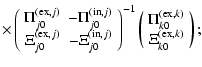 |
(18) |
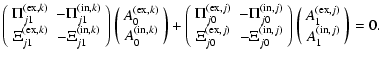
or equivalently:
| |
= | ||
 |
(19) |
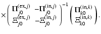
This can be solved straightforwardly by Cramer's rule:
| |
= |  |
(20) |
| = | 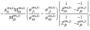 |
(21) | |
| = |  |
(22) |
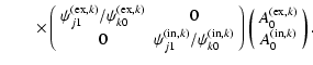
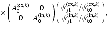
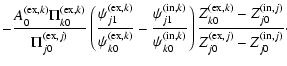
Here we have made use of the generalised impedance
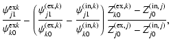
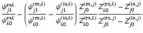
The impedances can be entirely expressed in terms of the Alfvén eigenvalues
Here and in what follows the upper sign applies for the internal expressions (with superscript
 |
(26) |
Thus the expressions for the ratios (23) and (24) can be expressed solely in terms of the Alfvén eigenvalues
| |
= | 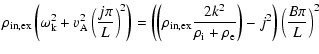 |
|
| = | 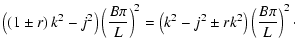 |
(27) |
Here r is a parameter related to the density contrast:
 |
(28) |
A fortiori we have:
 |
(29) |
and thus for the corrections to the eigenfunctions:
 |
(30) |
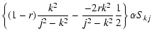
By use of the approximations for the impedances (25), the ratios (23) and (24) therefore become:
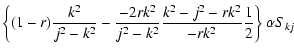


It is straightforward to check that Eq. (32) is equivalent to that obtained by Safari et al. (2007).
3 Discussion of the analytical results
The expressions for the amplitude ratios (31-32) nicely summarise the coupling of the different axial Fourier components in the kink-eigenfunctions in (weakly) stratified loops. In general
![]() is actually a shorthand notation for
is actually a shorthand notation for
![]() .
When a specific stratification is chosen which depends on a single stratification parameter, then in a linear expansion the alphas are simply proportional to the stratification parameter. If the stratification is sufficiently smooth,
.
When a specific stratification is chosen which depends on a single stratification parameter, then in a linear expansion the alphas are simply proportional to the stratification parameter. If the stratification is sufficiently smooth, ![]() quickly becomes smaller with n and retaining only the n=1 contribution is a fairly good approximation for many profiles. In fact for the specific profile of an exponential atmosphere with scale height H projected on a semicircular loop (as used by Andries et al. 2005a; Verth et al. 2007), all alphas except
quickly becomes smaller with n and retaining only the n=1 contribution is a fairly good approximation for many profiles. In fact for the specific profile of an exponential atmosphere with scale height H projected on a semicircular loop (as used by Andries et al. 2005a; Verth et al. 2007), all alphas except ![]() are second order and
are second order and
![]() .
.
The values of the first 6 coefficients of the sine expansions (linear in ![]() )
of the first 5 modes are summarised in Table 1. The diagonal entries are set to 1 and in absolute value at least a factor of 3 larger than the off-diagonal entries.
)
of the first 5 modes are summarised in Table 1. The diagonal entries are set to 1 and in absolute value at least a factor of 3 larger than the off-diagonal entries.
Table 1: Sine expansions of the first 5 eigenmodes (k) when expanded linearly in the stratification parameter.
Several interesting conclusions may be drawn, both from the table and from the expressions. Firstly, the contributions of the off-diagonal terms become stronger as k increases, both in displacement and compression. Hence, it seems that if higher order axial overtones could be detected, their potential for spatial seismology will be higher. Secondly, for the kth mode the largest coupling in the compression is always with the (k+2)th sine, while the (k-2)th contribution also becomes significant for higher k (and eventually of the same order). In the displacement it is the (k-2)th term that dominates with the (k+2)th sine almost of the same order (and dominating for k<3 as the (k-2)th term is absent there). Thus for the two modes observed so far (k=1,2) the behaviour can almost completely be characterised by the coupling with the third and fourth sine contribution respectively. Furthermore, the relative effect of longitudinal density stratification is always stronger in the compression than in the lateral displacement by a factor (k+2)2/k2. Hence the presence of the j=3 Fourier contribution in the fundamental oscillation is 9 times more pronounced in the total pressure perturbation than in the displacement, and the modifications to the first overtone are expected to be 4 times larger in the compression than in the displacement.
These results in terms of additional sine contributions in the eigenmodes can straightforwardly be related to the spatial shifts of the antinodes as investigated by Verth et al. (2007). From a linear expansion we find that the shift of the ith antinode can be approximated as:
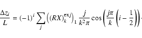
The results for all the antinodes of the first 5 modes are given in Table 2.
Table 2: Shift of the antinodes (i) of the first 5 eigenmodes (k) when expanded linearly in the stratification parameter.
Although for higher harmonics the contributions of the other Fourier modes increase, the shift of the antinodes remains roughly at the same order independent of the harmonic. It thus seems that the shifts of the antinodes are not the best signatures of the eigenmode modifications. Note that this is not due to the fact that the (k+2)th sine and the (k-2)th sine have opposite sign, as this is corrected for by the cosine factor in the expression for the shift (33). It can be argued that the shift should be normalised to the wavelength (varying as 1/k) and not to the length of the loop, in which case the conclusion would be that the shift increases linearly with k. From an observational point however it would be appropriate to normalise with respect to the resolution, which evidently does not depend on k. It can also be seen that the shift of the antinodes for the first overtone is as expected roughly about 4 times stronger in the compression than in the displacement. For higher harmonics the difference in the effect on displacement and compression also becomes smaller, as expected. However this does not follow the simple dependence (k+2)2/k2 derived above as the contributions from
The predicted shift in the antinode of the first overtone can be compared with the results by Verth et al. (2007). They normalise to half of the loop length and use L/H (thus actually L/2H) rather than ![]() as a stratification parameter, hence for comparison their proportionality constants should be multiplied by
as a stratification parameter, hence for comparison their proportionality constants should be multiplied by ![]() .
Their estimation based on the analytical model, which as in our treatment involves a linearisation in the stratification parameter, matches exactly with our results, and their numerical results deviated no more than 11% from that value.
.
Their estimation based on the analytical model, which as in our treatment involves a linearisation in the stratification parameter, matches exactly with our results, and their numerical results deviated no more than 11% from that value.
![\begin{figure}
\par\includegraphics[origin=rb,width=5cm,angle=90]{1481fig1a}\inc...
...1481fig1c}\includegraphics[origin=rb,width=5cm,angle=90]{1481fig1d}
\end{figure}](/articles/aa/full_html/2009/13/aa11481-08/img89.gif) |
Figure 1:
Shift of the antinodes as a function of the stratification
parameter |
| Open with DEXTER | |
![\begin{figure}
\includegraphics[origin=rb,width=5cm,angle=90]{1481fig2a}\include...
...1481fig2c}\includegraphics[origin=rb,width=5cm,angle=90]{1481fig2d}
\end{figure}](/articles/aa/full_html/2009/13/aa11481-08/img91.gif) |
Figure 2:
Shift of the antinodes as a function of the stratification parameter |
| Open with DEXTER | |
![\begin{figure}
\includegraphics[origin=rb,width=5cm,angle=90]{1481fig3a}\include...
...1481fig3c}\includegraphics[origin=rb,width=5cm,angle=90]{1481fig3d}
\end{figure}](/articles/aa/full_html/2009/13/aa11481-08/img92.gif) |
Figure 3:
Shift of the antinodes as a function of the period ratio P1/P2 and P1/P3 respectively. Dots correspond to the model with
|
| Open with DEXTER | |
4 Comparison with direct numerical computations
The correspondence with the results by Verth et al. (2007) is reassuring, but to gain even more confidence in the acquired results we have compared them with direct numerical eigenmode computations (i.e. non-linear in the stratification parameter) by means of the PDE2D code (Sewell 2005), a general-purpose partial differential equation solver. Figure 1 shows the shifts of the antinodes as a function of the stratification parameter
Also note that the figures indicate that the difference between the results of the two models is not only due to the non-linear relation between ![]() and
and ![]() but also because of the non-vanishing values of
but also because of the non-vanishing values of ![]() ,
,
![]() ,... This can be clearly seen by looking up, for a certain value of
,... This can be clearly seen by looking up, for a certain value of ![]() ,
the shifts for both displacement and compression (in Fig. 1), and then finding the corresponding values of
,
the shifts for both displacement and compression (in Fig. 1), and then finding the corresponding values of ![]() in the second model (through
Fig. 2). In this way the values for
in the second model (through
Fig. 2). In this way the values for ![]() are found to be different when considering displacement or compression. Hence, the results in the two models do not correspond through a simple mapping between the parameters
are found to be different when considering displacement or compression. Hence, the results in the two models do not correspond through a simple mapping between the parameters ![]() and
and ![]() .
.
With regard to the potential of using the observed eigenfunctions (or antinode shifts) the following question is pertinent. If the period ratio P2/P1 (or P3/P1) is observed accurately, does observation of the antinode shift allow us to discriminate between the two models? Hence Figs. 1 and 2 are repeated in Fig. 3 but as a function of the corresponding period ratio, which allows us to make a clear comparison between the different models, based on two observational parameters. As can be seen, a highly deviating period ratio is required before the antinode shifts between the models differ substantially. This is to be expected for the two models used here as they only differ in second order. Similarly in Fig. 4 the eigenfunctions are plotted. One curve represents the solution in the unstratified case, while the other two curves are the solutions in the two different models, where the stratification parameters are such that the resulting period ratios are equal in both models. Again it can be seen that the modifications are not significantly different between the two models considered. Much more significant differences between the models can only be expected if there is an important contribution of higher order sines in the stratification profile, hence if there aremore sudden longitudinal changes in the density, rather than the smooth profiles that are considered here.
![\begin{figure}
\includegraphics[origin=rb,width=5cm,angle=90]{1481fig4a}\include...
...1481fig4c}\includegraphics[origin=rb,width=5cm,angle=90]{1481fig4d}
\end{figure}](/articles/aa/full_html/2009/13/aa11481-08/img96.gif) |
Figure 4:
Eigenfunctions of the first ( upper panels) and second
( lower panels) overtones. Left is the displacement, right is the compression. Full lines correspond to the eigenfunctions obtained for the model
|
| Open with DEXTER | |
5 Conclusions
This paper is aimed at assessing the possibility that higher overtones of coronal loop kink modes might be more usefull for spatial seismology. By means of a linear expansion in the longitudinal stratification along with the ``thin tube'' approximation, the modifications to the eigenfunctions are calculated analytically. Simple and concise formulae are obtained, representing the jth Fourier contribution in the kth eigenmode. The results also provide a linear estimate of the shift of the antinodes. It is found that the higher overtones are indeed influenced even more than the first overtone, and that for the first overtones the influence is much stronger in the compression than in the transverse displacement. Also, the shift of the anti-nodes does not seem to be the best signature of the eigenmode modifications.The results are finally compared with direct numerical eigenmode computations. Although, the linear results give a good indication of the order of magnitude of the modifications, the deviations from the analytical predictions can certainly not be neglected under the expected coronal conditions. Although the results differ between models, it is clarified that if models are considered with smooth density profiles which hence have a dominant contribution from the fundamental sine in the stratification function, it is unlikely that the differences can be probed by the observational determination of the eigenfunctions. The numerical results indicate that the use of the eigenmode modifications as a tool to discriminate between two different but smooth density models requires both a very stratified equilibrium and a highly accurate determination of the anti-node shifts.
Acknowledgements
J.A. was supported by an International Outgoing Marie Curie Fellowship within the 7th European Community Framework Programme. I.A. acknowledges the support from the grant AYA2006-07637. M.G. acknowledges support from the grant GOA/2009-009.
References
- Andries, J., Arregui, I., & Goossens, M. 2005a, ApJ, 624, L57 [NASA ADS] [CrossRef] (In the text)
- Andries, J., Goossens, M., Hollweg, J., Arregui, I., & Van Doorsselaere, T. 2005b, A&A, 430, 1109 [NASA ADS] [CrossRef] [EDP Sciences] (In the text)
- Arregui, I., Van Doorsselaere, T., Andries, J., & Goossens, M. 2007, A&A, 463, 333 [NASA ADS] [CrossRef] [EDP Sciences] (In the text)
- De Moortel, I., & Brady, C. 2007, ApJ, 664, 1210 [NASA ADS] [CrossRef]
- Díaz, A. J., Oliver, R., & Ballester, J. L. 2002, ApJ, 580, 550 [NASA ADS] [CrossRef]
- Díaz, A. J., Oliver, R., Ballester, J. L., & Roberts, B. 2004, A&A, 424, 1055 [NASA ADS] [CrossRef] [EDP Sciences]
- Díaz, A. J., Oliver, R., & Ballester, J. 2006, ApJ, 645, 766 [NASA ADS] [CrossRef]
- Díaz, A. J., Donnelly, G. R., & Roberts, B. 2007, A&A, 476, 359 [NASA ADS] [CrossRef] [EDP Sciences]
- Donnelly, G. R., Díaz, A. J., & Roberts, B. 2006, A&A, 457, 707 [NASA ADS] [CrossRef] [EDP Sciences]
- Dymova, M., & Ruderman, M. 2005, Sol. Phys., 229, 79 [NASA ADS] [CrossRef] (In the text)
- Dymova, M., & Ruderman, M. 2006a, A&A, 459, 241 [NASA ADS] [CrossRef] [EDP Sciences]
- Dymova, M., & Ruderman, M. 2006b, A&A, 457, 1059 [NASA ADS] [CrossRef] [EDP Sciences]
- Edwin, P. M., & Roberts, B. 1983, Sol. Phys., 88, 179 [NASA ADS] [CrossRef] (In the text)
- Erdélyi, R., & Verth, G. 2007, A&A, 462, 743 [NASA ADS] [CrossRef] [EDP Sciences] (In the text)
- Goossens, M., Andries, J., & Aschwanden, M. 2002, A&A, 394, L39 [NASA ADS] [CrossRef] [EDP Sciences] (In the text)
- Goossens, M., Arregui, I., Ballester, J., & Wang, T. 2008, A&A, 484, 851 [NASA ADS] [CrossRef] [EDP Sciences] (In the text)
- Jess, D., Mathioudakis, M., Erdélyi, R., et al. 2008, ApJ, 680, 1523 [NASA ADS] [CrossRef] (In the text)
- McEwan, M., Donnelly, G., Díaz, A., & Roberts, B. 2006, A&A, 460, 893 [NASA ADS] [CrossRef] [EDP Sciences] (In the text)
- McEwan, M., Díaz, A., & Roberts, B. 2008, A&A, 481, 819 [NASA ADS] [CrossRef] [EDP Sciences]
- Nakariakov, V. M. 2000, in AIP Conf. Proc., 537, 264
- Nakariakov, V. M., & Ofman, L. 2001, A&A, 372, L53 [NASA ADS] [CrossRef] [EDP Sciences]
- Nakariakov, V. M., & Verwichte, E. 2005, Living Rev. Sol. Phys., 2, 3 [NASA ADS]
- Roberts, B. 2008, in IAU Symp., 247, 3
- Ruderman, M. S. 1992, J. Plas. Phys., 47, 175 [NASA ADS] [CrossRef] (In the text)
- Ruderman, M. S., & Roberts, B. 2002, ApJ, 577, 475 [NASA ADS] [CrossRef] (In the text)
- Ruderman, M. S., Verth, G., & Erdélyi, R. 2008, ApJ, 686, 694 [NASA ADS] [CrossRef] (In the text)
- Safari, H., Nasiri, S., & Sobouti, Y. 2007, A&A, 470, 1111 [NASA ADS] [CrossRef] [EDP Sciences]
- Sewell, G. 2005, The Numerical Solution of Ordinary and Partial Differential Equations (Wiley-Interscience) (In the text)
- Van Doorsselaere, T., Nakariakov, V., & Verwichte, E. 2007, A&A, 473, 959 [NASA ADS] [CrossRef] [EDP Sciences]
- Verth, G., & Erdélyi, R. 2008, A&A, 486, 1015 [NASA ADS] [CrossRef] [EDP Sciences] (In the text)
- Verth, G., Van Doorsselaere, T., Erdélyi, R., & Goossens, M. 2007, A&A, 475, 341 [NASA ADS] [CrossRef] [EDP Sciences] (In the text)
- Verth, G., Erdélyi, R., & Jess, D. B. 2008, ApJ, 687, L41 [NASA ADS] [CrossRef] (In the text)
- Verwichte, E., Nakariakov, V., Ofman, L., & Deluca, E. 2004, Sol. Phys., 223, 77 [NASA ADS] [CrossRef] (In the text)
Footnotes
- ...
![[*]](/icons/foot_motif.gif)
- Postdoctoral Fellow of the National Fund for Scientific Research- Flanders (Belgium) (FWO-Vlaanderen).
All Tables
Table 1: Sine expansions of the first 5 eigenmodes (k) when expanded linearly in the stratification parameter.
Table 2: Shift of the antinodes (i) of the first 5 eigenmodes (k) when expanded linearly in the stratification parameter.
All Figures
| |
Figure 1:
Shift of the antinodes as a function of the stratification
parameter |
| Open with DEXTER | |
| In the text | |
| |
Figure 2:
Shift of the antinodes as a function of the stratification parameter |
| Open with DEXTER | |
| In the text | |
| |
Figure 3:
Shift of the antinodes as a function of the period ratio P1/P2 and P1/P3 respectively. Dots correspond to the model with
|
| Open with DEXTER | |
| In the text | |
| |
Figure 4:
Eigenfunctions of the first ( upper panels) and second
( lower panels) overtones. Left is the displacement, right is the compression. Full lines correspond to the eigenfunctions obtained for the model
|
| Open with DEXTER | |
| In the text | |
Copyright ESO 2009
Current usage metrics show cumulative count of Article Views (full-text article views including HTML views, PDF and ePub downloads, according to the available data) and Abstracts Views on Vision4Press platform.
Data correspond to usage on the plateform after 2015. The current usage metrics is available 48-96 hours after online publication and is updated daily on week days.
Initial download of the metrics may take a while.