© The Authors 2026

1. Introduction

Measurements of stellar obliquities in binaries have shown that spin–orbit misalignment is a real and possibly common feature of binary-star dynamics. The archetypal system DI Herculis exhibits large stellar obliquities (Albrecht et al. 2009), while CV Velorum provides another well-studied case with a significantly misaligned stellar spin axis (Albrecht et al. 2014). Gaia-based population studies indicate that nonzero obliquity is not restricted to a few exceptional systems, and that a significant fraction of early-type binaries are misaligned (Marcussen et al. 2024; Smith et al. 2024). This picture is further strengthened by obliquity measurements in short-period low-mass eclipsing binaries (Spejcher et al. 2025). These results motivate renewed interest in dynamical pathways capable of creating, maintaining, or modifying stellar obliquities.

Most theoretical work considers primordial misalignment (e.g., Lai 2014), tertiary-driven evolution (e.g., Anderson et al. 2017), spin–orbit resonances involving circumbinary disks (e.g., Anderson & Lai 2021), or Cassini-state dynamics driven by nodal orbital precession (e.g., Felce & Fuller 2023). However, these works typically treat the two stellar spins as effectively uncoupled to first order, so that one or both stars may evolve into spin–orbit equilibria independently. By contrast, the possibility of a spin–spin resonance, which arises when the two stellar spin-precession frequencies become commensurate (e.g., Correia et al. 2016), has received no dedicated attention.

This question is especially relevant because the spin evolution of binary stars is shaped by both magnetic braking (e.g., Skumanich 1972) and tidal torques (e.g., Hut 1981). Their combined action has long been recognized as a key ingredient in binary evolution (e.g., Hurley et al. 2002; Repetto & Nelemans 2014) and has been revisited in both massive and low-mass binaries (Song et al. 2018; Fleming et al. 2019). Since the stellar spin-precession frequencies depend directly on the stellar rotation rates, their secular evolution can sweep binaries through the spin–spin commensurability. In this Letter, we isolate this resonance, characterize its dynamics, and assess its contribution to the observed diversity of spin–orbit angles in binary stars.

2. Spin dynamics

We consider a binary system composed of a primary and a secondary star, with masses m₀ and m₁, respectively, separated by the relative position vector r. Each star of mass m_i is modeled as an oblate ellipsoid with mean radius R_i, rotation period P_i, and angular velocity Ω_i = Ω_i s_i, where Ω_i = 2π/P_i and s_i is the axis of maximum inertia (gyroscopic approximation) with moment of inertia C_i = ζ_im_iR_i², where ζ_i is an internal structure constant. The rotational angular momentum of each star is then

$$\begin{array}{c}\hfill {\mathit{S}}_i=S_i{\mathit{s}}_i=C_i{\mathrm{\Omega }}_i{\mathit{s}}_i,\end{array}$$(1)

and the orbital angular momentum is

$$\begin{array}{c}\hfill \mathit{L}=L\mathit{k}=\beta n{a}^2\sqrt{1-e^2}\mathit{k},\end{array}$$(2)

where k is the unit vector normal to the orbital plane, a is the semi-major axis, e is the eccentricity, $n=\sqrt{\mu /a^3}$ is the mean motion, and β = m₀m₁/(m₀ + m₁) is the reduced mass.

The Hamiltonian of the system is (e.g., Smart 1953):

$$\begin{array}{c}\hfill H=\frac{{\mathit{p}}^2}{2\beta }-\frac{\beta \mu }{r}[1-{\displaystyle \sum _{i=0,1}}{J}_{2i}{\left(\frac{R_i}{r}\right)}^2{P}_2(\widehat{\mathit{r}}·{\mathit{s}}_i)]+{\displaystyle \sum _{i=0,1}}\frac{{\mathit{S}}_i^2}{2C_i},\end{array}$$(3)

where $\mathit{p}=\beta \dot{\mathit{r}}$, μ = G(m₀ + m₁), G is the gravitational constant, P₂(x) = (3x² − 1)/2 is the Legendre polynomial of degree two, and $\widehat{\mathit{r}}=\mathit{r}/r$ is the position unit vector; terms in (R_i/r)³ have been neglected (quadrupolar approximation). For the gravity-field coefficients, we adopt (e.g., Correia & Rodríguez 2013)

$$\begin{array}{c}\hfill J_{2i}=k_{2i}\frac{{\mathrm{\Omega }}_i^2{R}_i^3}{3G{m}_i},\end{array}$$(4)

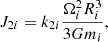
where k_2i is the second Love number for potential.

In general, the precession of the spin axes is much slower than the orbital motion. Since we are only concerned with spin–spin interactions, we average the Hamiltonian (Eq. (3)) over one orbital period. For the nonconstant terms, we obtain (e.g., Goldreich 1966; Boué & Laskar 2009)

$$\begin{array}{c}\hfill \overline{H}=-{\displaystyle \sum _{i=0,1}}\frac{{\alpha }_i}{2}{({\mathit{s}}_i·\mathit{k})}^2,\mathrm{with}{\alpha }_i=\frac{3G{m}_1{m}_0{J}_{2i}{R}_i^2}{2a^3{(1-e^2)}^{3/2}}·\end{array}$$(5)

In the averaged problem, all quantities in the Hamiltonian (Eq. (5)) are constant, except the unit vectors s_i and k, which can be related to the angular momentum components (Eqs. (1), (2)). The system’s secular evolution can therefore be described by the evolution of these components, derived from the Hamiltonian through Poisson brackets (e.g., Dullin 2004),

$$\begin{array}{cc}\hfill {\dot{\mathit{S}}}_i& =\{{\mathit{S}}_i,\overline{H}\}=\frac{\partial \overline{H}}{\partial {\mathit{S}}_i}\times {\mathit{S}}_i=-{\alpha }_i({\mathit{s}}_i·\mathit{k})\mathit{k}\times {\mathit{s}}_i,\hfill \end{array}$$(6)

$$\begin{array}{cc}\hfill \dot{\mathit{L}}& =\{\mathit{L},\overline{H}\}=\frac{\partial \overline{H}}{\partial \mathit{L}}\times \mathit{L}=-{\displaystyle \sum _{i=0,1}}{\alpha }_i({\mathit{s}}_i·\mathit{k}){\mathit{s}}_i\times \mathit{k}.\hfill \end{array}$$(7)

We verify that the norms of the individual angular momentum vectors are conserved, as is the total angular momentum,

$$\begin{array}{c}\hfill \mathit{J}=\mathit{L}+{\mathit{S}}_0+{\mathit{S}}_1=\mathrm{const}.\end{array}$$(8)

Following Boué & Laskar (2009), the equations of motion reduce to an integrable system. They can be simplified if we consider only the relative position in space of the unit vectors s_i and k, given by the direction cosines (Fig. A.1)

$$\begin{array}{c}\hfill x_i=cos{\theta }_i={\mathit{s}}_i·\mathit{k},\mathrm{and}z=cos\epsilon ={\mathit{s}}_0·{\mathit{s}}_1.\end{array}$$(9)

With these notations, we can rewrite the Hamiltonian (Eq. (5)),

$$\begin{array}{c}\hfill H_0={\alpha }_0{x}_0^2+{\alpha }_1{x}_1^2=-2\overline{H}=\mathrm{const},\end{array}$$(10)

and the total angular momentum (Eq. (8)),

$$\begin{array}{c}\hfill x_{★}=x_0+q{x}_1+{\delta }_{1}z=\frac{{\mathit{J}}^2-L^2-S_0^2-S_1^2}{2S_{0}L}=\mathrm{const},\end{array}$$(11)

with q = S₁/S₀ and δ_i = S_i/L.

3. Solutions in the precession frame

We now consider a frame (i₀, j₀, k) that follows the precession of s₀ about k, that is,

$$\begin{array}{c}\hfill {\mathit{i}}_0=\frac{{\mathit{s}}_0-x_0\mathit{k}}{{(1-x_0^2)}^{1/2}},{\mathit{j}}_0=\frac{\mathit{k}\times {\mathit{s}}_0}{{(1-x_0^2)}^{1/2}},\end{array}$$(12)

where j₀ is along the line of the nodes between the orbital plane and the equatorial plane of the star with mass m₀. In this frame, we can express s₁ = (u, v, x₁), for which

$$\begin{array}{c}\hfill u={\mathit{s}}_1·{\mathit{i}}_0=\frac{z-x_0{x}_1}{{(1-x_0^2)}^{1/2}}=sin{\theta }_{1}cos\mathrm{\Delta }\varphi ,\end{array}$$(13)

and

$$\begin{array}{c}\hfill v={\mathit{s}}_1·{\mathit{j}}_0=\frac{\mathit{k}·({\mathit{s}}_0\times {\mathit{s}}_1)}{{(1-x_0^2)}^{1/2}}=sin{\theta }_{1}sin\mathrm{\Delta }\varphi ,\end{array}$$(14)

with Δϕ = ϕ₁ − ϕ₀, where ϕ_i denotes the precession angle of s_i measured along the orbital plane (Fig. A.1). Because s₁ is a unit vector, we can also express

$$\begin{array}{c}\hfill x_1={\mathit{s}}_1·\mathit{k}={(1-u^2-v^2)}^{1/2}.\end{array}$$(15)

Following Correia (2016), we can get z from expression (13),

$$\begin{array}{c}\hfill z=x_0{x}_1+u{(1-x_0^2)}^{1/2},\end{array}$$(16)

while x₀ can be obtained by eliminating z in expression (11),

$$\begin{array}{c}\hfill (1+{\delta }_1{x}_1)x_0+{\delta }_{1}u{(1-x_0^2)}^{1/2}=x_{★}-q{x}_1,\end{array}$$(17)

which can be explicitly solved for x₀ as

$$\begin{array}{c}\hfill x_0=\frac{(1+{\delta }_1{x}_1)X(x_1,u)-{\delta }_{1}u\sqrt{1-X^2(x_1,u)}}{\sqrt{{(1+{\delta }_1{x}_1)}^2+{({\delta }_{1}u)}^2}},\end{array}$$(18)

with

$$\begin{array}{c}\hfill X(x_1,u)=\frac{x_{★}-q{x}_1}{\sqrt{{(1+{\delta }_1{x}_1)}^2+{({\delta }_{1}u)}^2}}·\end{array}$$(19)

Thus, x₀ depends only on (x₁, u), and hence on (u, v) (Eq. (15)); so does the Hamiltonian (Eq. (10)),

$$\begin{array}{c}\hfill H_0=H_0(x_1,u,x_{★})=H_0(u,v,x_{★}).\end{array}$$(20)

In Fig. 1, we show the secular trajectories for the spin of the secondary projected on the orbital plane in the TOI-2119 binary system (Table B.1) when P₀ ≈ P₁ = 2 day. These trajectories were obtained by plotting the level curves H₀(u, v, x_★) = const (Eq. (20)), but they correspond to the integration of the secular Equations (6) and (7) for different initial values of θ₁.

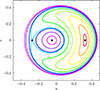Fig. 1. Secular trajectories in the TOI-2119 system (Table B.1) adopting P0 = 2.1 day and P1 = 2.0 day. We show the spin axis of the secondary, s1, projected on the orbital plane. These trajectories are obtained by plotting the level curves H0(u, v, x★) = const (Eq. (20)). The stationary solutions (Cassini states) are marked with a dot.

The dynamics is akin to that of a second fundamental model for resonance (Henrard & Lemaître 1983). In astronomy, such behavior occurs for spin–orbit (e.g., Ward & Hamilton 2004; Correia 2015) or mean–motion resonances (e.g., Delisle et al. 2012; Petit 2021). Here, the resonant motion corresponds to a commensurability between the precession frequencies of the two stellar spins, ${\dot{\varphi }}_0\approx {\dot{\varphi }}_1$, with (Eq. (6))

$$\begin{array}{c}\hfill {\dot{\varphi }}_i=-{\alpha }_i{x}_i/S_i;\end{array}$$(21)

that is, it corresponds to a spin–spin resonance.

4. Cassini states

Cassini states are stationary equilibria of the spin axis (Correia 2015) given by the extrema of the Hamiltonian (Eq. (20)),

$$\begin{array}{c}\hfill \frac{\partial H_0}{\partial u}=0\mathrm{and}\frac{\partial H_0}{\partial v}=0.\end{array}$$(22)

Since H₀ = H₀(x₁, u), we have

$$\begin{array}{c}\hfill \frac{\partial H_0}{\partial v}=\frac{\partial H_0}{\partial x_1}\frac{\partial x_1}{\partial v}=-\frac{\partial H_0}{\partial x_1}\frac{v}{x_1}=0.\end{array}$$(23)

We therefore conclude that v = 0 is always a possible equilibrium solution (equivalent to Δϕ = 0 or π), where the unit vectors s₀, s₁, and k remain coplanar. We denote these coplanar states by u_c = ±sin θ_c (Eq. (13)), which are given by (Eq. (10))

$$\begin{array}{c}\hfill {\frac{\partial H_0}{\partial u}|}_{v=0}=-2{\alpha }_{1}u+2{\alpha }_0{x}_0{\frac{\partial x_0}{\partial u}|}_{v=0}=0.\end{array}$$(24)

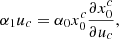
Setting v = 0 in x₁ (Eq. (15)), we get ${x_1}^c=\sqrt{1-{u_c}^2}$, and for x₀ (Eq. (18)), we have x₀^c = x₀(x₁^c, u_c). Equation (22) therefore provides an implicit condition for the coplanar states,

$$\begin{array}{c}\hfill {\alpha }_1{u}_c={\alpha }_0{x}_0^c\frac{\partial x_0^c}{\partial u_c},\end{array}$$(25)

whose roots can be found in the interval u_c ∈ [ − 1, 1] using numerical methods. In Appendix C, we provide approximate analytic expressions for these states when S₁ ≪ L.

In the example shown in Fig. 1, the stationary solutions correspond to three Cassini states, u_c = −0.275, u_c = −0.0522, and u_c = 0.323, equivalent to θ₁ ≈ −16.0°, θ₁ ≈ −3.0°, and θ₁ ≈ 18.9°, respectively. The smallest θ₁ value corresponds to a hyperbolic unstable point, but the spin can be stabilized in the other two states. The largest θ₁ value lies within a libration region and thus corresponds to the resonant equilibrium.

In Fig. 2, we plot the Cassini states as a function of the rotation period of the primary, P₀, for the TOI-2119 system (Table B.1) with P₁ = 2 day. For P₀ ≲ 2 day, we observe that there is only one stable state at nearly zero obliquity. For P₀ ≳ 2 day, the obliquity of the previous state increases to high values, while two additional states appear. This is a consequence of the emergence of a separatrix that introduces a libration region around the high-obliquity state (Fig. 1). We then conclude that when the rotation period of the primary increases (e.g., through magnetic braking), the spins can be captured into resonance, leading to significant changes in the obliquity.

Fig. 2. Cassini states as a function of the rotation period of the primary, P0, for the TOI-2119 system (Table B.1) with P1 = 2 day. These equilibria are obtained by solving Eq. (25). The vertical dashed line corresponds to the configuration shown in Fig. 1.

5. Obliquity excitation

So far, we have neglected magnetic braking and tidal torques, which modify the rotational angular momenta, S_i (Eq. (1)). These effects extract energy from the system, so the problem is no longer integrable and must be solved numerically. In Appendices D and E, we provide the secular equations for magnetic braking and tidal effects, respectively.

As an example, we consider the TOI-2119 binary system (Doyle et al. 2025), composed of an M-type main-sequence primary and a brown dwarf secondary (Table B.1). Observational studies of young brown dwarfs with masses in the range 0.02 − 0.08 m_⊙ show rotation periods spanning 0.7 − 4.5 day, with a median value of 1.9 day, and a clear trend of longer periods at higher mass (Scholz et al. 2018). Likewise, population studies of young low-mass stars in the range 0.15 − 1.5 m_⊙ show a rotation period distribution of 0.2 − 30 day, peaking near 2 day, with M stars rotating faster on average than GK stars (Rebull et al. 2018). We therefore adopt an initial period of P₀ = 1 day for the primary and P₁ = 2 day for the secondary. For the initial obliquities, we use the currently observed value θ₀ = 15.7° for the primary and arbitrarily set θ₁ = 1° for the secondary.

In Fig. 3 (left), we show the secular spin evolution of both stars under magnetic braking alone. The rotation period of the secondary is not expected to change significantly because it is a brown dwarf (e.g., Zapatero Osorio et al. 2006). Thus, as the rotation period of the primary increases and reaches P₀ ≈ P₁ = 2 day, the precession rates also become comparable, ${\dot{\varphi }}_0\approx {\dot{\varphi }}_1$ (Eq. (21)), thereby modifying the phase space (Fig. 2). The spin of the brown dwarf, initially circulating around the only existing Cassini state (red state in Fig. 2), adiabatically follows this state, leading to a significant increase in its obliquity. In the absence of tides, this increase is permanent and can drive the obliquity to values close to 90° for P₀ ≫ 2 day.

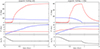Fig. 3. Secular spin evolution of the TOI-2119 binary stars as a function of time. We show the obliquity (top), rotation period (middle), and precession frequency ratio (bottom). The primary and secondary spins are shown in blue and red, respectively. The left column shows the evolution under magnetic braking alone, while the right column also includes tidal effects for both stars.

The obliquity of the primary, θ₀, is also affected by the resonance crossing. Because the total angular momentum is nearly conserved and S_i ≪ L, we generally have (Eq. (11))

$$\begin{array}{c}\hfill cos{\theta }_0+qcos{\theta }_1\approx \mathrm{const}.\end{array}$$(26)

It follows that θ₀ must decrease as θ₁ increases. For the TOI-2119 system, the decrease in θ₀ is small since q ≪ 1 as well.

In Fig. 3 (right), we show the secular spin evolution including tides for both stars. There are two main differences relative to the previous case. First, tides also modify the secondary rotation period, driving it toward the pseudo-synchronous equilibrium at P₁ = 4.2 day (Eq. (E.5)) and thus delaying the resonance encounter. Second, tides act directly on the obliquity, damping it to near zero (e.g., Correia et al. 2016). As a result, although the secondary’s obliquity, θ₁, is still excited by the spin–spin resonance, the primary’s obliquity, θ₀, continues to decrease owing to tides. Once θ₀ is damped to nearly zero, the resonant equilibrium can no longer be maintained, and θ₁ is also damped.

In Appendix F, we provide another example of a stellar binary with two main-sequence stars, EBLM J2025-45. In this case both stars undergo magnetic braking, which may give rise to complementary obliquity excitation behaviors in the absence of tides. However, when tides are included, the system evolves in a way very similar to TOI-2119 (Figs. F.2 and F.3).

6. Discussion

In this Letter, we studied the dynamics of spin–spin coupling in stellar binaries and its effect on their obliquities. We showed that this mechanism can efficiently excite the obliquity of the secondary to high values even when the primary’s obliquity is small. However, the resonant equilibrium breaks down as the primary’s obliquity nears zero, owing to tidal dissipation.

Magnetic braking is the main driver of high-obliquity states, while tidal damping acts against it. Although magnetic braking is well constrained by observational studies (e.g., Gallet & Bouvier 2013), tidal dissipation in stars relies mostly on theoretical models and can vary by orders of magnitude depending on stellar properties and age (e.g., Ogilvie 2014; Mathis 2015). More efficient tidal damping may prevent high-obliquity states from developing, whereas weaker dissipation may allow such states to survive over the system’s lifetime.

The two examples shown, TOI-2119 and EBLM J2025-45, are compact binaries (a ≲ 0.07 au), where tides are more efficient. In wider binaries, magnetic braking is expected to dominate the evolution, allowing high-obliquity states to persist longer. However, the precession rates are then also slower (Eq. (21)), making the resonant excitation less efficient.

Spin–spin resonances are most likely to occur during the early stages of stellar evolution, when rotation is rapid and evolves quickly, but the resulting high-obliquity states may persist for Gyr. In our examples, we adopted initial rotation periods near resonance, so that the resonance crossing occurs after a short time. Larger initial period ratios may delay or prevent the onset of obliquity excitation.

Our results show that spin–spin coupling may play an important role in shaping the diversity of spin–orbit angles observed in young stellar binary systems.

Acknowledgments

We acknowledge support from FCT – Fundação para a Ciência e a Tecnologia, I.P., Portugal, through the CFisUC project UID/04564/2025 (with DOI identifier 10.54499/UID/04564/2025).

References

Appendix A: Reference angles definition

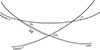Fig. A.1. Reference planes for the definition of the direction cosines.

Appendix B: Parameters of the binary systems

Appendix C: Cassini states for S₁ ≪ L

For binary systems, we usually have (Eqs. (1), (2)),

$$\begin{array}{c}\hfill {\delta }_1=\frac{S_1}{L}=\frac{C_1{\mathrm{\Omega }}_1}{\beta n{a}^2\sqrt{1-e^2}}\approx {\zeta }_1{\left(\frac{R_1}{a}\right)}^2\ll 1.\end{array}$$(C.1)

Then, neglecting terms in qδ₁ and δ₁², we rewrite Eq. (18) as

$$\begin{array}{c}\hfill x_0\approx x_{★}-q{x}_1-{\delta }_1(x_{★}{x}_1+u{(1-x_{★}^2)}^{1/2}),\end{array}$$(C.2)

and so

$$\begin{array}{c}\hfill {\frac{\partial x_0}{\partial u}|}_{v=0}\approx qu/x_1+{\delta }_1(x_{★}u/x_1-{(1-x_{★}^2)}^{1/2}).\end{array}$$(C.3)

Replacing in Eq. (25), we get for the Cassini states

$$\begin{array}{c}\hfill {\alpha }_1{u}_c{x}_1^c\approx {\alpha }_0(x_{★}-q{x}_1^c)[q{u}_c+{\delta }_1(x_{★}{u}_c-x_1^c{(1-x_{★}^2)}^{1/2})],\end{array}$$(C.4)

where ${x_1}^c=\sqrt{1-{u_c}^2}$. This is a quartic equation in u_c, which may have up to four real roots. To find them, we can use the trigonometric relations,

$$\begin{array}{c}\hfill u_c=sin{\theta }_c,x_1^c=cos{\theta }_c,\mathrm{and}{x}_{★}=cos{\theta }_{★},\end{array}$$(C.5)

where θ_★ corresponds approximately to the initial θ₀ (Eq. (11)). Replacing in Eq. (C.4), we get for the Cassini states,

$$\begin{array}{c}\hfill \frac{{\alpha }_1}{{\alpha }_0}sin{\theta }_{c}cos{\theta }_c\approx (cos{\theta }_{★}-qcos{\theta }_c)[qsin{\theta }_c+{\delta }_{1}sin({\theta }_c-{\theta }_{★})],\end{array}$$(C.6)

whose approximate roots are

$$\begin{array}{c}\hfill {\theta }_c\approx arctan\left(\frac{{\delta }_{1}sin{\theta }_{★}(q\pm cos{\theta }_{★})}{{\alpha }_1/{\alpha }_0+q^2\pm qcos{\theta }_{★}}\right),\end{array}$$(C.7)

and

$$\begin{array}{c}\hfill {\theta }_c\approx \pm arccos\left(\frac{qcos{\theta }_{★}}{{\alpha }_1/{\alpha }_0+q^2}\right).\end{array}$$(C.8)

We also conclude that the high-obliquity states (Eq. (C.8)) are only possible when

$$\begin{array}{c}\hfill {\alpha }_1/{\alpha }_0\ge q(cos{\theta }_{★}-q).\end{array}$$(C.9)

Appendix D: Magnetic braking

A star’s magnetic field couples to its surrounding ionized wind. As the wind escapes, it extracts angular momentum from the star, causing its rotation to slow down over time. This process, known as magnetic braking, is particularly important in low- and intermediate-mass stars, which possess substantial convective envelopes and are therefore able to sustain efficient magnetic dynamos. The efficiency of magnetic braking is commonly parametrized in terms of the convective turnover timescale, τ_i, which depends on stellar mass¹.

For 0.08 < m_i/m_⊙ < 1.36, we adopt (Wright et al. 2018)

$$\begin{array}{c}\hfill {log}_{10}{\tau }_i=2.33-1.50\left(\frac{m_i}{m_{\odot }}\right)+0.31{\left(\frac{m_i}{m_{\odot }}\right)}^2,\end{array}$$(D.1)

where τ_i is expressed in days. For m_i > 1.36 m_⊙, the convective turnover timescale decreases steeply. Stellar evolution models indicate that it drops by approximately two orders of magnitude for m_i ∼ 2 m_⊙ (e.g., Amard et al. 2019).

The efficiency of magnetic braking also depends sensitively on the Rossby number, ℛ_i = P_i/τ_i. When the Rossby number falls below a critical threshold, ℛ, several indicators of magnetic activity appear to saturate, reaching an approximately constant maximum value that is largely independent of ℛ_i. Following Matt et al. (2015), we write ℛ = ℛ_⊙/χ, where ℛ_⊙ is the solar Rossby number and χ ≈ 10.

The magnetic-braking torque can then be written, for rapidly rotating stars in the saturated regime (ℛ_i < ℛ_S), as

$$\begin{array}{c}\hfill {\dot{\mathit{S}}}_i=-{\dot{S}}_{\odot }{\left(\frac{R_i}{R_{\odot }}\right)}^{3.1}{\left(\frac{m_i}{m_{\odot }}\right)}^{0.5}{\chi }^2\left(\frac{{\mathrm{\Omega }}_i}{{\mathrm{\Omega }}_{\odot }}\right){\mathit{s}}_i,\end{array}$$(D.2)

whereas for more slowly rotating stars in the unsaturated regime (ℛ_i > ℛ_S), we use

$$\begin{array}{c}\hfill {\dot{\mathit{S}}}_i=-{\dot{S}}_{\odot }{\left(\frac{R_i}{R_{\odot }}\right)}^{3.1}{\left(\frac{m_i}{m_{\odot }}\right)}^{0.5}{\left(\frac{{\tau }_i}{{\tau }_{\odot }}\right)}^2{\left(\frac{{\mathrm{\Omega }}_i}{{\mathrm{\Omega }}_{\odot }}\right)}^3{\mathit{s}}_i,\end{array}$$(D.3)

where τ_⊙ ≈ 12.9 days is the solar convective turnover timescale, and ${\dot{S}}_{\odot }\approx 6.3\times {10}^{23}$ J ≈1.4 × 10⁻¹⁴ m_⊙ au² yr⁻² is a constant calibrated against observations.

Appendix E: Tidal evolution

Tidal effects arise from the differential and inelastic deformation of each star under the gravitational forcing of its companion. Because the stars are not perfectly rigid, this perturbation produces a distortion that gives rise to a tidal bulge. The dissipation of mechanical energy inside the star introduces a time delay, Δt, between the initial perturbation and the resulting deformation. As a consequence, the companion exerts a torque on the tidal bulge, which modifies the spin and the orbit.

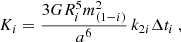
The exact dependence of Δt on the frequency of the tidal perturbation is unknown, because it depends on stellar properties and age (e.g., Ogilvie 2014). For simplicity, we adopt here a model with constant Δt, which can be made linear (Singer 1968; Hut 1981). The equations of motion are (e.g., Correia 2009)

$$\begin{array}{cc}& {\dot{\mathit{S}}}_i=-n{K}_i[f_1(e)\frac{{\mathit{s}}_i+cos{\theta }_i\mathit{k}}{2}\frac{{\mathrm{\Omega }}_i}{n}-f_2(e)\mathit{k}],\hfill \end{array}$$(E.1)

$$\begin{array}{cc}& \dot{\mathit{L}}={\displaystyle \sum _{i=0,1}}n{K}_i[f_1(e)\frac{{\mathit{s}}_i+cos{\theta }_i\mathit{k}}{2}\frac{{\mathrm{\Omega }}_i}{n}-f_2(e)\mathit{k}],\hfill \end{array}$$(E.2)

$$\begin{array}{cc}& \dot{a}={\displaystyle \sum _{i=0,1}}\frac{2K_i}{\beta a}[f_2(e)cos{\theta }_i\frac{{\mathrm{\Omega }}_i}{n}-f_3(e)],\hfill \end{array}$$(E.3)

with

$$\begin{array}{c}\hfill K_i=\frac{3G{R}_i^5{m}_{(1-i)}^2}{a^6}{k}_{2i}\mathrm{\Delta }{t}_i,\end{array}$$(E.4)

and e² = 1 − L²/(β²μa), f₁(e) = (1 + 3e² + 3e⁴/8)/(1 − e²)^9/2, f₂(e) = (1 + 15e²/2 + 45e⁴/8 + 5e⁶/16)/(1 − e²)⁶, f₃(e) = (1 + 31e²/2 + 255e⁴/8 + 185e⁶/16 + 25e⁸/64)/(1 − e²)^15/2.

Tidal dissipation in stars can vary by several orders of magnitude (e.g., Mathis 2015). Observational constraints on the mean tidal quality factor in eclipsing binaries suggest 10⁵ ≲ Q ≲ 10⁷ (e.g., Patel et al. 2023), while the distribution of close-in exoplanets around Sun-mass stars gives Q ≳ 10⁷ (e.g., Penev et al. 2012). We therefore assume here Δt_i = 0.05 sec for m_i < 0.8 m_⊙ and Δt_i = 0.005 sec for m_i > 0.8 m_⊙, which correspond to Q_i ≈ 10⁶ and Q_i ≈ 10⁷, respectively, using Q_i⁻¹ = nΔt_i.

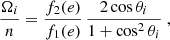
The equilibrium spin is reached when ${\dot{\mathit{S}}}_i=0$ (Eq. (E.1)), that is, for (e.g., Correia 2009)

$$\begin{array}{c}\hfill \frac{{\mathrm{\Omega }}_i}{n}=\frac{f_2(e)}{f_1(e)}\frac{2cos{\theta }_i}{1+{cos}^2{\theta }_i},\end{array}$$(E.5)

which is also known as pseudo-synchronous rotation. The corresponding timescale is τ_spin ∼ C_i/K_i, whereas for the circularization of the orbit we get τ_orb ∼ βa²/K_i. For both systems in Table B.1, we obtain τ_spin ∼ 1 Gyr for the primary, τ_spin ∼ 100 Myr for the secondary, and τ_orb ∼ 100 Gyr.

Appendix F: Application to EBLM J2025-45

As a complementary example of obliquity excitation, we consider here the EBLM J2025-45 binary system (Spejcher et al. 2025), which is composed of a Sun-like G-type primary and an M-type secondary main-sequence stars (Table B.1).

For guidance, in Fig. F.1, we plot the Cassini states for the EBLM J2025-45 system as a function of the rotation period ratio, P₀/P₁. This picture is similar to that of TOI-2119 (Fig. 2). For P₀/P₁ ≲ 1, there is only one stable state at nearly zero obliquity. For P₀/P₁ ≳ 1, the obliquity of the original state increases to high values, while two additional states appear.

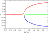Fig. F.1. Cassini states as a function of the rotation period ratio, P0/P1, for the EBLM J2025-45 system (Table B.1) with P1 = 2 day. These equilibria are obtained by solving Eq. (25).

Observational studies of young low-mass stars in the range 0.15 − 1.5 m_⊙ show rotation periods spanning 0.2 − 30 day, peaking near 2 day (Rebull et al. 2018). In a first experiment, we thus adopt initial rotation periods of P₀ = 1.5 day for the primary and P₁ = 2.0 day for the secondary (Fig. F.2). In a second experiment, we swap these values, adopting P₀ = 2.0 day for the primary and P₁ = 1.5 day for the secondary (Fig. F.3). For the initial obliquities, we use the currently observed value θ₀ = 17.3° for the primary and arbitrarily set θ₁ = 5° for the secondary.

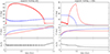Fig. F.2. Secular spin evolution of the EBLM J2025-45 binary stars as a function of time, starting with P0 = 1.5 day and P1 = 2.0 day. We show the obliquity (top), rotation period (middle), and precession frequency ratio (bottom). The primary and secondary spins are shown in blue and red, respectively. The left column shows the evolution under magnetic braking alone, while the right column also includes tidal effects for both stars.

In Fig. F.2 (left), we show the secular spin evolution of both stars under magnetic braking alone. We initially have P₀ < P₁ and the rotation period of the secondary, P₁, varies more slowly than that of the primary, P₀. As a result, the rotation periods of both stars become equal after a short time, bringing the system into resonance. The obliquity of the secondary, θ₁, then increases, following the high-obliquity Cassini state (red state in Fig. F.1), while the obliquity of the primary, θ₀, decreases (Eq. (26)). The obliquity of the secondary peaks around 60°, corresponding to a maximum period ratio P₀/P₁. As the G-type star spins down, it enters the unsaturated regime, where magnetic braking is less efficient (Eq. (D.3)). At that point, the ratio P₀/P₁ begins to decrease, also leading to a decrease in θ₁ (red state in Fig. F.1). When P₀/P₁ < 1, the system moves out of resonance, since there is only one Cassini state left.

In Fig. F.2 (right), we show the secular spin evolution including tides for both stars. Tides raised in the secondary are very efficient, so its rotation period increases much faster than in the absence of tides. Yet, after some time, the secondary’s rotation period stabilizes at P₁ = 6.2 day, near the pseudo-synchronous equilibrium (Eq. (E.5)), allowing it to be caught up with the primary’s rotation period. Then, the system enters in resonance, and θ₁ is excited, while θ₀ decreases owing to tides. Once θ₀ is damped to nearly zero, the resonant equilibrium can no longer be maintained, and θ₁ is also damped in a way very similar to that observed for the TOI-2119 system (Fig. 3).

In Fig. F.3 (left), we show the secular spin evolution of both stars under magnetic braking alone. In this case, we initially have P₀ > P₁, and so there is no resonance crossing at early times. However, as the G-type star enters the unsaturated regime, the evolution of its rotation period slows down, allowing P₁ to catch up with P₀. At that point, the system crosses the resonance, but with a decreasing ratio P₀/P₁. That is, before the resonant encounter, the system circulates around a low-obliquity Cassini state (green state in Fig. F.1). Then, this state disappears, and the system must circulate around the only remaining Cassini state (red state in Fig. F.1). Nevertheless, although in this case resonant capture is not possible, the obliquity of the secondary is still slightly excited by about 5°.

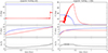Fig. F.3. Secular spin evolution of the EBLM J2025-45 binary stars as a function of time, starting with P0 = 2.0 day and P1 = 1.5 day. We show the obliquity (top), rotation period (middle), and precession frequency ratio (bottom). The primary and secondary spins are shown in blue and red, respectively. The left column shows the evolution under magnetic braking alone, while the right column also includes tidal effects for both stars.

In Fig. F.3 (right), we show the secular spin evolution including tides for both stars. Although we initially have P₀ > P₁, tides raised in the secondary allow P₁ to increase faster than P₀. The system then crosses the resonance with an increasing ratio P₀/P₁, allowing resonant capture and subsequent excitation of θ₁. Once θ₀ is damped to nearly zero owing to tides, the resonant equilibrium is broken, and θ₁ is also damped in a way very similar to that observed for the TOI-2119 system (Fig. 3).

All Tables

All Figures

	Fig. 1. Secular trajectories in the TOI-2119 system (Table B.1) adopting P0 = 2.1 day and P1 = 2.0 day. We show the spin axis of the secondary, s1, projected on the orbital plane. These trajectories are obtained by plotting the level curves H0(u, v, x★) = const (Eq. (20)). The stationary solutions (Cassini states) are marked with a dot.
In the text

	Fig. 2. Cassini states as a function of the rotation period of the primary, P0, for the TOI-2119 system (Table B.1) with P1 = 2 day. These equilibria are obtained by solving Eq. (25). The vertical dashed line corresponds to the configuration shown in Fig. 1.
In the text

	Fig. 3. Secular spin evolution of the TOI-2119 binary stars as a function of time. We show the obliquity (top), rotation period (middle), and precession frequency ratio (bottom). The primary and secondary spins are shown in blue and red, respectively. The left column shows the evolution under magnetic braking alone, while the right column also includes tidal effects for both stars.
In the text

	Fig. A.1. Reference planes for the definition of the direction cosines.
In the text

	Fig. F.1. Cassini states as a function of the rotation period ratio, P0/P1, for the EBLM J2025-45 system (Table B.1) with P1 = 2 day. These equilibria are obtained by solving Eq. (25).
In the text

Fig. F.2. Secular spin evolution of the EBLM J2025-45 binary stars as a function of time, starting with P0 = 1.5 day and P1 = 2.0 day. We show the obliquity (top), rotation period (middle), and precession frequency ratio (bottom). The primary and secondary spins are shown in blue and red, respectively. The left column shows the evolution under magnetic braking alone, while the right column also includes tidal effects for both stars.

In the text

Fig. F.3. Secular spin evolution of the EBLM J2025-45 binary stars as a function of time, starting with P0 = 2.0 day and P1 = 1.5 day. We show the obliquity (top), rotation period (middle), and precession frequency ratio (bottom). The primary and secondary spins are shown in blue and red, respectively. The left column shows the evolution under magnetic braking alone, while the right column also includes tidal effects for both stars.

In the text

References

- Albrecht, S., Reffert, S., Snellen, I. A. G., & Winn, J. N. 2009, Nature, 461, 373 [Google Scholar]
- Albrecht, S., Winn, J. N., Torres, G., et al. 2014, ApJ, 785, 83 [CrossRef] [Google Scholar]
- Amard, L., Palacios, A., Charbonnel, C., et al. 2019, A&A, 631, A77 [NASA ADS] [CrossRef] [EDP Sciences] [Google Scholar]
- Anderson, K. R., & Lai, D. 2021, ApJ, 906, 17 [Google Scholar]
- Anderson, K. R., Lai, D., & Storch, N. I. 2017, MNRAS, 467, 3066 [NASA ADS] [CrossRef] [Google Scholar]
- Boué, G., & Laskar, J. 2009, Icarus, 201, 750 [CrossRef] [Google Scholar]
- Claret, A. 2023, A&A, 674, A67 [NASA ADS] [CrossRef] [EDP Sciences] [Google Scholar]
- Correia, A. C. M. 2009, ApJ, 704, L1 [NASA ADS] [CrossRef] [Google Scholar]
- Correia, A. C. M. 2015, A&A, 582, A69 [NASA ADS] [CrossRef] [EDP Sciences] [Google Scholar]
- Correia, A. C. M. 2016, MNRAS, 457, L49 [Google Scholar]
- Correia, A. C. M., & Rodríguez, A. 2013, ApJ, 767, 128 [NASA ADS] [CrossRef] [Google Scholar]
- Correia, A. C. M., Boué, G., & Laskar, J. 2016, Celest. Mech. Dyn. Astron., 126, 189 [NASA ADS] [CrossRef] [Google Scholar]
- Delisle, J.-B., Laskar, J., Correia, A. C. M., & Boué, G. 2012, A&A, 546, A71 [NASA ADS] [CrossRef] [EDP Sciences] [Google Scholar]
- Doyle, L., Cañas, C. I., Libby-Roberts, J. E., et al. 2025, MNRAS, 536, 3745 [Google Scholar]
- Dullin, H. R. 2004, Reg. Chaot. Dynam., 9, 255 [Google Scholar]
- Felce, C., & Fuller, J. 2023, MNRAS, 526, 6168 [Google Scholar]
- Fleming, D. P., Barnes, R., Davenport, J. R. A., & Luger, R. 2019, ApJ, 881, 88 [Google Scholar]
- Gallet, F., & Bouvier, J. 2013, A&A, 556, A36 [NASA ADS] [CrossRef] [EDP Sciences] [Google Scholar]
- Goldreich, P. 1966, Rev. Geophys. Space Phys., 4, 411 [Google Scholar]
- Henrard, J., & Lemaître, A. 1983, Celest. Mech., 30, 197 [NASA ADS] [CrossRef] [Google Scholar]
- Hurley, J. R., Tout, C. A., & Pols, O. R. 2002, MNRAS, 329, 897 [Google Scholar]
- Hut, P. 1981, A&A, 99, 126 [NASA ADS] [Google Scholar]
- Lai, D. 2014, MNRAS, 440, 3532 [NASA ADS] [CrossRef] [Google Scholar]
- Leconte, J., Lai, D., & Chabrier, G. 2011, A&A, 528, A41 [NASA ADS] [CrossRef] [EDP Sciences] [Google Scholar]
- Marcussen, M. L., Albrecht, S. H., Winn, J. N., et al. 2024, ApJ, 975, 149 [Google Scholar]
- Mathis, S. 2015, A&A, 580, L3 [EDP Sciences] [Google Scholar]
- Matt, S. P., Brun, A. S., Baraffe, I., Bouvier, J., & Chabrier, G. 2015, ApJ, 799, L23 [Google Scholar]
- Ogilvie, G. I. 2014, ARA&A, 52, 171 [Google Scholar]
- Patel, R., Penev, K., & Schussler, J. 2023, MNRAS, 524, 5575 [Google Scholar]
- Penev, K., Jackson, B., Spada, F., & Thom, N. 2012, ApJ, 751, 96 [NASA ADS] [CrossRef] [Google Scholar]
- Petit, A. C. 2021, Celest. Mech. Dyn. Astron., 133, 39 [NASA ADS] [CrossRef] [Google Scholar]
- Rebull, L. M., Stauffer, J. R., Cody, A. M., et al. 2018, AJ, 155, 196 [Google Scholar]
- Repetto, S., & Nelemans, G. 2014, MNRAS, 444, 542 [NASA ADS] [CrossRef] [Google Scholar]
- Scholz, A., Moore, K., Jayawardhana, R., et al. 2018, ApJ, 859, 153 [NASA ADS] [CrossRef] [Google Scholar]
- Sethi, R., Martin, D. V., Barker, A. J., et al. 2026, MNRAS, 547, stag454 [Google Scholar]
- Singer, S. F. 1968, Geophys. J. R. Astron. Soc., 15, 205 [Google Scholar]
- Skumanich, A. 1972, ApJ, 171, 565 [Google Scholar]
- Smart, W. M. 1953, Celestial Mechanics (London, New York: Longmans, Green) [Google Scholar]
- Smith, C. L., Moe, M., & Kratter, K. M. 2024, ApJ, 975, 153 [Google Scholar]
- Song, H. F., Meynet, G., Maeder, A., et al. 2018, A&A, 609, A3 [NASA ADS] [CrossRef] [EDP Sciences] [Google Scholar]
- Spejcher, B., Martin, D. V., Pandina, J., et al. 2025, ArXiv e-prints [arXiv:2511.23430] [Google Scholar]
- Ward, W. R., & Hamilton, D. P. 2004, AJ, 128, 2501 [Google Scholar]
- Wright, N. J., Newton, E. R., Williams, P. K. G., Drake, J. J., & Yadav, R. K. 2018, MNRAS, 479, 2351 [Google Scholar]
- Zapatero Osorio, M. R., Martín, E. L., Bouy, H., et al. 2006, ApJ, 647, 1405 [NASA ADS] [CrossRef] [Google Scholar]
The convective turnover timescale is the time required for a convective element to traverse the stellar convection zone.