


| Issue |
A&A
Volume 710, June 2026
|
|
|---|---|---|
| Article Number | A369 | |
| Number of page(s) | 17 | |
| Section | Stellar structure and evolution | |
| DOI | https://doi.org/10.1051/0004-6361/202659849 | |
| Published online | 29 June 2026 | |
Characterizing six seismic solar analogs observed by Kepler, K2, and HERMES
1
Université Paris-Saclay, Université Paris Cité, CEA, CNRS, AIM, 91191 Gif-sur-Yvette, France
2
Instituto de Astrofísica de Canarias (IAC), E-38205 La Laguna, Tenerife, Spain
3
Universidad de La Laguna (ULL), Departamento de Astrofísica, E-38206 La Laguna, Tenerife, Spain
4
School of Physics and Astronomy, University of Birmingham, Birmingham B15 2TT, UK
5
Department of Physics and Astronomy, Uppsala University, Box 516, SE-751 20 Uppsala, Sweden
6
STAR Institute, Université de Liège, Liège, Belgium
7
Department of Astronomy, Yale University, PO Box 208101 New Haven, CT 06520-8101, USA
8
Center for Solar-Stellar Connections, WDRC, 9020 Brumm Trail, Golden, CO 80403, USA
9
Department of Astronomical Science, School of Physical Sciences, SOKENDAI, 2-21-1 Osawa, Mitaka, Tokyo 181-8588, Japan
10
Solar Science Observatory, National Astronomical Observatory of Japan, 2-21-1 Osawa, Mitaka, Tokyo 181-8588, Japan
11
Center for Space Science, New York University Abu Dhabi, PO Box 129188 Abu Dhabi, UAE
12
Astronomical Institute of Charles University, V Holešovičkách 2 Prague 18000, Czech Republic
13
Université Paris Cité, Université Paris-Saclay, CEA, CNRS, AIM, 91191 Gif-sur-Yvette, France
14
INAF – Osservatorio Astrofisico di Catania, Via S. Sofia, 78, 95123 Catania, Italy
15
IMT Atlantique, F-29238 Brest, France
16
Ecole Centrale-Supelec, Université Paris-Saclay, 91190 Gif-sur-Yvette, France
17
ENS Paris-Saclay, Université Paris-Saclay, 91190 Gif-sur-Yvette, France
18
Stellar Astrophysics Centre, Department of Physics and Astronomy, Aarhus University, Ny Munkegade 120, DK-8000 Aarhus C, Denmark
★ Corresponding author: This email address is being protected from spambots. You need JavaScript enabled to view it.
Received:
13
March
2026
Accepted:
20
April
2026
Abstract
Solar analogs–stars that closely match the fundamental properties of the Sun–provide key benchmarks for testing stellar structure and evolution across different ages and activity levels. Their detailed characterization helps place the Sun into context within the broader population of solar-like stars. This study presents the characterization of six seismic solar analogs observed by the NASA Kepler and K2 missions. Combining asteroseismic constraints from space-based photometry with high-resolution spectroscopy and Gaia astrometry, we derived their fundamental parameters and assessed their resemblance to the Sun. Global seismic properties and individual oscillation modes were extracted from the photometric light curves, while atmospheric parameters were obtained from data collected by the High-Efficiency and High-Resolution Mercator Echelle Spectrograph (HERMES) at the Mercator telescope. Stellar modeling using seven independent stellar evolution codes yielded consistent masses, radii, and ages. These stars have masses between 0.91 and 1.04 M⊙, radii between 0.95 and 1.08 R⊙, and ages from about 1.8–9.1 Gyr, with typical systematic uncertainties of ±0.02 M⊙, ±0.01 R⊙, and ±0.7 Gyr, respectively. One star, EPIC 206064678, exhibits properties very similar to those of the Sun, with M = 1.016 ± 0.033 M⊙, R = 0.990 ± 0.011 R⊙, and an age of 5.40 ± 0.12 Gyr. It can therefore be considered a close solar twin, although it is slightly older and more metal-rich (0.25 ± 0.07 dex). Four targets display binarity signatures and all exhibit very low chromospheric activity. This work broadens the sample of well-characterized seismic solar analogs toward a larger sample of metallicities and ages, providing new references for comparative stellar studies and future asteroseismic investigations.
Key words: stars: evolution / stars: oscillations / stars: solar-type
© The Authors 2026
 Open Access article, published by EDP Sciences, under the terms of the Creative Commons Attribution License (https://creativecommons.org/licenses/by/4.0), which permits unrestricted use, distribution, and reproduction in any medium, provided the original work is properly cited.
This article is published in open access under the Subscribe to Open model. This email address is being protected from spambots. You need JavaScript enabled to view it. to support open access publication.
1. Introduction
The Sun is the cornerstone of stellar astrophysics, providing an unparalleled benchmark for the study of stars because of its proximity and the extraordinary detail with which it can be characterized. Its unique status enables investigations of stellar structure and dynamics with a precision unattainable for any other star. However, solar observations provide only a snapshot of the 4.5 Gyr evolution of our star, leaving fundamental questions unresolved such as to what extent the Sun is a typical ∼1 M⊙ solar-like star, what its history is, and what its future looks like.
For decades, astronomers have searched for stars with physical properties closely matching those of the Sun, leading to the concepts of solar twins (e.g., Cayrel de Strobel et al. 1981; Cayrel de Strobel & Bentolila 1989) and solar analogs (e.g., Hardorp 1978; Cayrel de Strobel 1996). Solar twins are stars whose effective temperature (Teff), surface gravity (log g), metallicity ([Fe/H]), micro-turbulence, photometric properties, chemical composition, age, luminosity, rotation, and magnetic fields are indistinguishable from those of the Sun within observational uncertainties. Because of these stringent criteria, true solar twins are rare, with only about a hundred identified despite extensive observational campaigns (e.g., Yana Galarza et al. 2021 and references therein). Their close spectroscopic similarity to the Sun nevertheless makes them powerful laboratories for differential abundance analyses, tests of stellar evolution models, and calibrations of stellar parameters. Notable examples include 18 Sco (Bazot et al. 2012, 2018), HIP 102152, and CoRoT ID 102684698 (do Nascimento et al. 2013).
Solar analogs form a broader class of Sun-like stars that do not need to reproduce all solar properties. They are typically defined within a mass range of 0.9 ≤ M/M⊙ ≤ 1.1, without constraints on age, allowing a wider diversity of stellar parameters. This flexibility enables solar analogs to represent different evolutionary stages of Sun-like stars and to span a range of rotation rates, magnetic activity levels, and chemical compositions (e.g., do Nascimento et al. 2014, 2020; Salabert et al. 2016a; Metcalfe et al. 2016, 2022; Beck et al. 2017; García 2017; Carvalho-Silva et al. 2025; Galarza et al. 2025). Their study is therefore crucial for reconstructing a “Sun-in-time” sequence and for exploring how stellar evolution depends on parameters such as metallicity. Examples include KIC 10644253 (Salabert et al. 2016b), a younger and more active solar analog, KIC 8006161 (Karoff et al. 2018), a younger and more metal-rich star, and the binary system 16 Cyg A/B (Metcalfe et al. 2012; Davies et al. 2015), which represents an older counterpart.
A major advance in the characterization of solar-like stars has come from asteroseismology–the study of stellar oscillations. Space missions such as the Convection, Rotation, and planetary Transits mission (CoRoT; Baglin et al. 2006; Auvergne et al. 2009); Kepler/K2 (Borucki et al. 2009; Howell et al. 2014); and more recently the Transiting Exoplanet Survey Satellite (TESS; Ricker et al. 2014) have enabled the detection of solar-like oscillations in hundreds of main-sequence stars. These observations provide precise measurements of stellar masses, radii, and ages (Barban et al. 2009; Ballot et al. 2011; Lund et al. 2017; Mathur et al. 2022), surpassing what is achievable from the ground (e.g., Bedding et al. 2010). When combined with high-resolution spectroscopy, asteroseismic analyses yield the most accurate stellar parameters currently attainable (Lebreton & Goupil 2014; Grossmann et al. 2025). They have also led to the identification of seismic solar analogs, defined as stars whose global seismic parameters–the frequency of maximum power, νmax, and the large frequency separation, Δν (e.g., García & Ballot 2019)–are within 10% of the solar reference values. These stars offer the opportunity to probe the internal structure of Sun-like stars with high precision, although they are not necessarily solar analogs in the classical spectroscopic definition.
Expanding the sample of seismic solar analogs is therefore essential for placing the Sun in a broader stellar context, yet only a few such stars have been characterized (e.g., Salabert et al. 2016b; Karoff et al. 2018; Huber et al. 2022). In this paper, we report a combined seismic and spectroscopic analysis of six additional seismic solar analogs observed by Kepler/K2, High-Efficiency and High-Resolution Mercator Echelle Spectrograph (HERMES; Raskin et al. 2011), and Gaia (Gaia Collaboration 2016). The layout of the paper is as follows. Section 2 describes the Kepler and K2 observations. Sections 3, 4, and 5 present the seismic analysis, multiplicity, and spectroscopic analysis. Stellar structure and evolutionary models are presented in Sect. 7. Finally, Sect. 8 discusses the results and summarizes our conclusions.
2. Observations
From a pre-analysis of Kepler and K2 observations, we selected six seismic solar analogs with global seismic parameters, extracted from the A2Z pipeline (Mathur et al. 2010), lying within 10% of the solar references (3050 and 135 μHz for νmax and Δν, respectively). The first star, KIC 3241581, was observed for one month in short cadence (Gilliland et al. 2010) by Kepler (Mathur et al. 2022), and was also extensively spectroscopically characterized with HERMES (Beck et al. 2016) on the Mercator telescope. We used Kepler Simple Aperture Photometry flux (SAPflux) light curves corrected by the Kepler Asteroseismic Data Analysis and Calibration Software (KADACS1) described in García et al. (2011), which were filtered with a high-pass filter with a cutoff at three days and gap-filled using a multiscale, discrete cosine transform following inpainting techniques (García et al. 2014; Pires et al. 2015).
The remaining five targets were observed by the K2 mission in short-cadence mode. Three of them, namely EPIC 206064678, EPIC 206245055, and EPIC 206371648, were observed during Campaign C32, while EPIC 212624487 was observed during Campaign C6. The fifth target, EPIC 212708252, was observed in two campaigns, C6 and C17, and was analyzed following the same methodology as described in González-Cuesta et al. (2023). A search for signatures of a possible magnetic activity cycle in EPIC 212708252 was carried out by Berloff et al. (2026), but no statistically significant evidence was found. In addition, EPIC 212708252 and EPIC 212624487 were previously analyzed by Lund et al. (2024), who derived their global seismic parameters, and by Hookway et al. (2025), the authors of which characterized their individual oscillation modes. For all K2 targets, we adopted light curves from the Ecliptic Plane Input Catalog Variability Extraction and Removal for Exoplanet Science Targets pipeline (EVEREST3; Luger et al. 2016, 2018). The light curves were subsequently gap-filled using the same procedure applied to the Kepler target. HERMES spectroscopy was obtained for all the targets. To reach high signal-to-noise ratios (S/Ns), the observations were split into multiple integrations, typically spanning ∼400 days. This also allowed for the search of binarity signatures (see Sect. 5).
3. Data analysis
Two complementary seismic analyses were done for each target. First, we extracted the global seismic parameters that describe the overall oscillation pattern of the star. Second, we characterized the individual oscillation modes through detailed peak-bagging procedures using two independent fitting codes.
3.1. Extracting global seismic parameters
We analyzed the power spectral densities (PSDs) of the six targets using A2Z. This pipeline identifies the regular spacing of oscillation modes in the PSD by computing the power spectrum of the power spectrum, from which Δν is determined. The background is modeled as the sum of several components: a power law to account for magnetic activity, two Harvey-like profiles (Harvey 1985) representing different convective timescales, and a constant white-noise term to take into account the contribution of the photon noise. νmax is then derived by fitting a Gaussian envelope to the background-corrected PSD. A second inference of the seismic global parameters as well as the phase offset, ϵ, is obtained using the universal pattern module of the apollinaire package (see the details in Breton et al. 2022). The results from A2Z and apollinaire are summarized in Table 1. As expected, the values of the two global seismic parameters, Δν and νmax, obtained with both pipelines, are consistent within 1σ for all stars.
Seismic and spectroscopic parameters of the six seismic solar analogs.
3.2. Characterizing individual modes: Peak-bagging
To characterize the individual oscillation modes, we applied two independent peak-bagging pipelines: the apollinaire module and PBjam (Nielsen et al. 2021, 2025). These tools were used to fit and extract the mode frequencies, amplitudes, and line widths from the observed PSDs. The following subsections describe the implementation and fitting strategies adopted for each method and present the resulting frequency lists used for the stellar modeling.
3.2.1. apollinaire
The apollinaire module4 implements an ensemble Markov chain Monte Carlo (MCMC) approach using the emcee sampler (Foreman-Mackey et al. 2013). Each oscillation mode, identified by its radial order (n) and angular degree (ℓ), is modeled as a symmetric Lorentzian profile characterized by its central frequency (νn, ℓ), linewidth (Γn, ℓ), and height (Hn, ℓ). In practice, the parameters sampled by the MCMC procedure are νn, ℓ, log An, 0, logΓn, ℓ, and the mode visibility ratios (Vℓ). The mode amplitudes, An, ℓ = VℓAn, 0, are related with the other mode properties as  (e.g., Lund et al. 2017). This parameterization ensures uniform prior distributions and facilitates efficient convergence of the MCMC chains. The likelihood is constructed assuming that the statistical fluctuations of the observed power spectrum about the model follow a χ2 distribution with two degrees of freedom.
3.2.2. PBjam
The mode characterization was also carried out using PBjam, following a two-stage approach consisting of (1) mode identification based on asymptotic relations, and (2) a detailed peak-bagging analysis. During the mode identification stage, we applied a background model to the power spectrum composed of three Harvey-like profiles (Harvey 1985) and a white-noise component. This background was then combined with a model of the ℓ = 0, 1, and 2 oscillation modes, each represented as the sum of Lorentzian profiles (Anderson et al. 1990). The mode frequencies were constrained by the asymptotic relation for p modes, in which the parameters Δν, νmax, and ε and the small separations δν01 and δν02 were treated as free parameters. The number of radial orders included in the model was varied between 6 and 14, depending on the S/N of the power spectrum. The Dynesty nested sampling algorithm (Speagle 2020) was used to sample the posterior probability distribution of the model parameters, and thereby determine the most probable mode frequencies. The prior distribution was constructed from a large dataset of thousands of previously analyzed stars and stellar models, allowing empirical knowledge of stellar oscillations to inform the mode identification posterior.
The results from the mode identification were then passed to the second stage of PBjam, corresponding to the detailed peak bagging. In this step, each oscillation mode was fitted individually, allowing for rotational splitting and acoustic glitches not captured in the asymptotic approximation. Normal priors were applied to the mode frequencies, logarithmic heights, and logarithmic line widths, with prior widths of 3% of Δν for the frequencies and 50% of the mode identification values for the heights and widths. The fitting procedure was performed using the emcee MCMC sampler. Finally, to validate the results, we computed the ratio between the median absolute deviation (MAD) of the posterior and prior distributions for each mode frequency. Modes with a ratio below 50% were deemed to contain new information from the observed light curve, and only these modes were retained.
3.2.3. Consolidated peak-bagging results
The peak-bagging results for each star are presented in Appendix A. For each star, there is a table listing the radial order, n, and the angular degree, ℓ, of the detected modes, along with their frequencies and symmetrized uncertainties derived from the two fitting methods. We compared the agreement between the two pipelines and found that their frequencies agreed within 1σ for 74.5% of the modes across all targets.
4. Binarity of the targets
About 50% of main-sequence, solar-like stars with spectral types from late F to early K are expected to be in multiple systems (e.g., Lada 2006; Moe & Di Stefano 2017), whereas this fraction decreases to about 30% for solar-like pulsating stars (e.g., Beck 2026). Stars in close binary systems may undergo tidal and magnetic interactions that can affect their oscillation modes (e.g., García et al. 2010; Chaplin et al. 2011; Mathur et al. 2019; Gaulme et al. 2014, 2020; Gehan et al. 2024). It is therefore important to assess the multiplicity and the orbital separations between the stars for our stellar sample. Indeed, since we used stellar evolution codes that assume single-star evolution, it is important to know whether the inferred stellar parameters could be biased.
Four out of the six target stars are reported to be members of binary or multiple stellar systems (see Table 2). A companion to EPIC 206064678 was detected via speckle interferometry at a separation of 0.8 arcseconds and a position angle of approximately 300 degrees. The companion is fainter by 3.2 magnitudes in the I band (Horch et al. 2010; Tokovinin et al. 2020). This binary is also resolved by Gaia, which reports an angular separation of 0.814 arcseconds and a consistent position angle. Although the companion lacks parallax and proper motion measurements in Gaia data release 3 (DR3), the relatively high proper motion of EPIC 206064678, combined with the reasonably long time baseline between the interferometric and Gaia observations (> 8 years), makes a chance alignment with a background star highly unlikely. If the two objects were not co-moving, a significant shift in relative position would be expected. Assuming a distance of 57.6 pc (from the inverse of the Gaia DR3 parallax), the projected physical separation was estimated to be ∼47 au, suggesting an orbital period of several hundred years. However, the current time span of interferometric observations is insufficient to derive a reliable orbital solution.
Photometric, RV, and astrometric information of the six candidate solar analogs.
The star EPIC 206371648 is listed in the 9th Catalog of Spectroscopic Binary Orbits (SB9; Pourbaix et al. 2004) under entries SBC9 3701 and SBC9 3702. Tokovinin (2018) identified EPIC 206371648 as a hierarchical triple system, consisting of an inner spectroscopic binary with a period of 111.1 days and an outer visual companion with an orbital period of 18 440 ± 1576 days (∼50.49 ± 4.3 years) and eccentricity of e = 0.451 ± 0.044. These parameters were derived from extensive speckle interferometric data. Videla et al. (2022) derived a mass ratio of ∼0.52–0.96 between the inner pair and the outer companion, depending on the input data. The system shows a high renormalized unit weight error (RUWE ≃ 9.1) in Gaia DR3 (an RUWE higher than ∼1.25 indicates either multiplicity or a poor astrometric solution; Penoyre et al. 2022), yet no solution is present in the Gaia DR3 Non-Single Star (NSS) catalog (Gaia Collaboration 2023a), in either the two-body orbit tables (TBOs) or nonlinear proper motion tables (NLACs). The star is also flagged as a double-lined spectroscopic binary (SB2) candidate in Zheng et al. (2023) based on Large Sky Area Multi-ObjectFiber Spectroscopic Telescope (LAMOST; Zhao et al. 2012; Zong et al. 2020) spectra and machine-learning classification. However, the apparent SB2 signature may result from the combined light of the outer companion and one of the inner components rather than an actual double-lined spectroscopic nature of the inner pair. The asymmetry in the cross-correlation function (CCF) observed by Tokovinin (2018) at some epochs was explained in this way. Although the absorption lines of the secondary component are hardly distinguishable in the spectrum, we were able to estimate the maximum contribution of the secondary component to the spectral analysis of the primary, assuming that the secondary component is a main-sequence star. We found that the change in the effective temperature was not significant within the measured uncertainties. Only the metallicity and v sin i were affected by the secondary contribution, resulting in an increase in metallicity of up to 0.05 dex and a decrease in velocity of ∼2 km/s. As these values were comparable within 1σ of the original measurements, we decided to retain them.
The star EPIC 212708252 was identified as a long-period spectroscopic binary with  days (≃167 years) based on 25 years of radial-velocity (RV) monitoring with CORALIE (Barbato et al. 2023). The orbit is highly eccentric (e∼ 0.73), with a peak-to-peak RV amplitude of ∼4 km/s. The RUWE is moderate (∼1.3), and no solution is listed in either TBO or NLAC, as expected for a system with such a long orbital period. However, the system shows a significant proper motion anomaly (Kervella et al. 2019), consistent with its binary nature.
Finally, KIC 3241581 was reported to be a binary by Beck et al. (2016). The system appears in the Gaia DR3 NSS catalog with an acceleration solution and a relatively high RUWE ∼ 6. This target was continuously monitored with the HERMES spectrograph (Raskin et al. 2011), mounted on the 1.2-meter Mercator Telescope at the Roque de los Muchachos Observatory in La Palma, Canary Islands, Spain. These 40 observations over 2303 days enabled further constraints on its orbital parameters. Using the radial code5, we analyzed the RVs from HERMES monitoring to refine the orbital elements. The resulting parameters are listed in Table B.1, and the orbital fit is shown in Fig. B.1.
From this analysis we conclude that the periods of the companions are long. As a consequence the oscillating star can be treated as a single star without tidal interaction that would affect the oscillation mode pattern (Gaulme et al. 2014; Beck et al. 2024).
5. Atmospheric parameters
To ensure a consistent dataset of fundamental parameters, high-resolution spectra were collected for each target using the HERMES spectrograph. It has a spectral resolution of R ∼ 85 000 over a wavelength range spanning 375–900 nm. The wavelength calibration was achieved using a thorium-argon-neon (ThArNe) emission lamp.
Observations were carried out between June 2019 and August 2020, except for EPIC 212708252 and KIC 3241581, which have been followed up with the same spectrograph since 2012 and thus cover a longer time range as detailed in Tables 1 and 2. The spectroscopic data were reduced using the instrument’s dedicated pipeline (Raskin et al. 2011). These observations are part of a large follow-up program focused on seismic solar-analog stars, described in detail in Beck et al. (2016, 2017). The RV for individual spectra was calculated via the CCF with a standard G2-mask across the wavelength range of 478–653 nm, as implemented in the HERMES data-reduction toolbox. For this observational setup, the spectrograph’s night-to-night RV stability at the 3σ level is approximately 300 m/s, a conservative threshold often used to identify binary systems. To ensure RV stability, several ThArNe reference frames were taken throughout the night between science exposures.
The combined stellar spectra were analyzed using the 1D/local thermodynamic equilibrium (LTE) Brussels Automatic Code for Characterizing High accUracy Spectra (BACCHUS; Masseron et al. 2016; Hayes et al. 2022) with the model atmospheres in radiative and convective scheme (MARCS; Gustafsson et al. 2008) and atomic and molecular line lists from Heiter et al. (2021). The effective temperature was determined requiring no trend between the abundances of Fe I lines and their excitation potentials. The surface gravity was obtained from ionization balance between Fe I and Fe II, while the microturbulent velocity was derived by removing trends between Fe-line abundances and equivalent widths. The metallicity corresponds to the mean abundance of the Fe I lines. The code simultaneously fits the Fe-line profiles with a mean line-broadening parameter. The projected rotational velocity (v sin i) was estimated assuming that this broadening results from the quadratic sum of instrumental resolution (R = 85 000), macroturbulence following Doyle et al. (2014) for G–K main-sequence stars, and rotational broadening. For slow rotators, v sin i derived in this way remains uncertain because of degeneracies with macroturbulence, possible instrumental resolution variations, and uncertainties in line parameters. In addition, the spectral energy distribution of each star was analyzed with the virtual observatory spectral energy distribution analyzer VOSA tool (Bayo et al. 2008). The resulting temperatures are fully consistent with those from the spectroscopic analysis. As a final check, the wings of the Hα and Mg I triplet lines, which are sensitive to temperature and pressure, were visually inspected. Once the stellar parameters were fixed, lithium abundances (or upper limits) were derived from the 6707 Å line. The resulting stellar properties are listed in Table 2.
We note that our stars are not solar analogs in the classical spectroscopic sense (e.g., Cayrel de Strobel 1996). Indeed, the target selection was based purely on the global seismic parameters as explained in Sect. 2. This corresponds to an extended version of the classical definition of solar analogs as the stars have Teff within 300 K of the solar value and [Fe/H] within 0.4 dex, similarly to those in Salabert et al. (2016a).
We completed the spectroscopic analysis by computing the S-index following Beck et al. (2016, multiplied by 23 to match the Mount Wilson Observatory scale) and the log R′HK(B − V) index following Suárez Mascareño et al. (2015) for each individual exposure of the HERMES spectra. We note that low-activity indicators are especially sensitive to systematic measurement errors. Consequently, values below the solar mean activity level – ∼0.17 for the S-index (Egeland et al. 2017) and −4.91 for the log R′HK(B − V) (Mamajek & Hillenbrand 2008) – should be interpreted with caution, particularly when comparing different studies, spectral types, or instruments.
We also calculated the Ca II infrared-triplet (IRT) index following the approach of Godoy-Rivera et al. (2026a). In brief, the  index was computed from the activityindex_espcs parameter (α) in the gaiadr3.astrophysical_parameters table, which quantifies the excess equivalent width with respect to a reference spectrum at the Ca II IRT as observed by the Gaia Radial Velocity Spectrometer (Lanzafame et al. 2023). Out of the six targets in our sample, four of them have measured equivalent widths with positive values, where a
  could be calculated, as well as a S/N of α/σα > 3. The values of both indices are given in Table 2.
A detailed analysis of KIC 3241581 can be found in Beck et al. (2016). Here, we obtained results that were highly consistent with our previous results, although with somewhat larger uncertainties. This difference arises because the previous study employed a differential approach with respect to the Sun, which leads to improved accuracy. Nevertheless, for the sake of consistency across our sample, we adopted our own values for the modeling.
For completeness, we searched for stellar parameters of our targets in several spectroscopic surveys: Apache Point Observatory Galactic Evolution Experiment (APOGEE DR17; Majewski et al. 2017; Abdurro’uf et al. 2022), LAMOST (DR10; Cui et al. 2012; Zhao et al. 2012) Medium- and Low-Resolution Spectroscopy (MRS and LRS, respectively), Gaia-European Southern Observatory (Gaia-ESO, v5.1; Gilmore et al. 2012; Randich et al. 2013; Hourihane et al. 2023), Galactic Archaeology with HERMES (GALAH DR4; De Silva et al. 2015; Buder et al. 2025), and Gaia DR3 gspspec (Gaia Collaboration 2023b; Recio-Blanco et al. 2023). We also queried the spectro-photometric catalog of Andrae et al. (2023), which used the XGBoost algorithm on the Gaia DR3 XP coefficients to derive stellar parameters.
Out of our six targets, we found two in common with APOGEE, four in common with Gaia DR3 gspspec, one in common with LAMOST LRS, and five in common with Andrae et al. (2023). No overlap was found with the LAMOST MRS, Gaia-ESO, or GALAH surveys. The Andrae et al. (2023) values are by construction on the APOGEE scale. Following Godoy-Rivera et al. (2025), for the Gaia DR3 general stellar parametrizer spectroscopy (gspspec) values we only considered the best-quality data and implemented the gravity and metallicity calibration to place them on a common scale with other surveys (Recio-Blanco et al. 2023).
Figure 1 shows the comparison6 of the spectroscopic surveys versus the HERMES values. The five targets in common with Andrae et al. (2023) and the two targets in common with APOGEE show a good overall agreement with HERMES. Regarding the four targets in common with Gaia DR3 gspspec (green) and the one target in common with LAMOST LRS, while the temperature and metallicity differences are moderate, the surface gravities are substantially underestimated (Δlog(g)≳0.2 dex) for all of them, hinting at systematic errors. Because we only have HERMES spectra for all the targets and to ensure homogeneity, we adopted those spectroscopic values throughout this work.
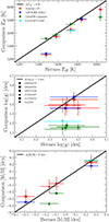 |
Fig. 1. Comparison of atmospheric parameters: HERMES versus spectroscopic surveys. The top, middle, and bottom panels show the comparison of effective temperatures, surface gravities, and metallicities. The HERMES values are on the x-axis, and the spectroscopic surveys are on the y-axis, with Andrae et al. (2023) in red, APOGEE DR17 in blue, and Gaia DR3gspspec in green. Each target is shown by a different symbol, as indicated in the middle panel legend. The Andrae et al. (2023) values show the better overall agreement, and largest overlap, with HERMES. |
6. Luminosity computation
We calculated luminosities following the approach of Godoy-Rivera et al. (2026b), which we briefly summarize here. First, we calculated absolute magnitudes in the G band using the Gaia DR3 astrometric and photometric information (Lindegren et al. 2021; Gaia Collaboration 2023b), accounting for the parallax and extinction corrections as in Godoy-Rivera et al. (2025). Second, we used the gaiadr3_bcg7 function (Creevey et al. 2023), which interpolates MARCS models (Gustafsson et al. 2008) taking the atmospheric parameters from Table 1 as input, and we calculated G-band bolometric corrections by sampling one thousand Monte Carlo realizations of each target. Third, we combined these absolute magnitudes and bolometric corrections with the solar bolometric magnitude from Mamajek et al. (2015) to compute the luminosities. We validated our values by comparing them with those of Gaia DR3 final luminosity age mass estimator (FLAME), which reported luminosities for four (out of six) of our targets, finding that in all four cases both estimates agree at the 3σ-level.
As some of our targets are members of multiple systems, we tested the impact of companions on the derived luminosities. For this, we compared the aforementioned Gaia-based luminosities (which would include the contribution of companions unresolved by Gaia) with the values that can be estimated from the asteroseismic scaling relations (which would only include the brightest oscillating component, L ∝ νmax2Δν−4Teff5). The comparison between both estimates agree within 1σ for four out of the six targets, with the remaining two targets agreeing at the 1.3 and 1.5 σ-levels (EPIC 212708252 and EPIC 206371648, respectively). Thus, we conclude that unresolved companions do not strongly impact the Gaia-based luminosities.
7. Stellar modeling
We modeled the stars to estimate the masses, radii, and ages of the targets. We used several methods and stellar evolution codes, allowing us to measure the systematics. The input parameters of the optimizing codes were the atmospheric parameters from HERMES (Teff and [Fe/H]), luminosity from Gaia, the global seismic parameters (Δν and νmax), and the individual frequencies of the modes. We note that no correction from the line-of-sight velocity of the stars was applied. Since they are negligible compared to the uncertainties reported, we do not expect any impact, as also shown by Davies et al. (2014).
7.1. IACgrid description
The IACgrid is composed of models computed with the Modules for Experiments in Stellar Astrophysics (MESA, Paxton et al. 2011, 2013, 2015) stellar evolution code (version 15140). It uses standard input physics with Opacity Project at Livermore (OPAL) opacities (Iglesias & Rogers 1996) and chemical mixture from Grevesse & Sauval (1998). The masses are in the range of 0.8 M⊙ to 1.5 M⊙ (with a step of 0.01 M⊙), initial abundances from −0.3 to 0.4 dex (with a step of 0.05 dex), and mixing length parameter αmlt between 1.5 and 2.2 (with a step of 0.05). The mixing length follows the prescription of Cox & Giuli (1968). The frequencies were computed with the Aarhus adiabatic oscillation package ADIPLS (Christensen-Dalsgaard 2008a). The primordial helium abundance was taken as Y0 = 0.249. Based on the Galactic chemical evolution model with ΔY/ΔZ fixed to 1.33, we took an initial solar helium abundance of 0.2744 and initial solar metallicity of 0.0191. These values are consistent with the opacities and chemical abundances used in the models.
The optimization relies on a χ2 minimization, where the χ2 is divided into the spectroscopic one, the frequencies one, and the dynamical one. To compare the observed frequencies to the model ones, we applied surface corrections following Pérez Hernández et al. (2019). The uncertainties are estimated via Monte Carlo simulations, assuming Gaussian uncertainties on the observables. More details on the optimization and the computation of the uncertainties on the derived parameters can be found in Pérez Hernández et al. (2019) and González-Cuesta et al. (2023).
7.2. BASTA
The BASTA results were obtained using the Bayesian framework of the Bayesian STellar Algorithm (see Aguirre Børsen-Koch et al. 2022), which infers stellar properties from a custom-computed grid of stellar models. This grid, generated with the Garching Stellar Evolution Code (garstec; Weiss & Schlattl 2008), contains evolutionary tracks constructed under well-established input physics. The equation of state combines contributions from the OPAL group (Rogers et al. 1996; Rogers & Nayfonov 2002) and the Mihalas–Hummer–Däppen formulation (Mihalas et al. 1988; Hummer & Mihalas 1988; Daeppen et al. 1988; Mihalas et al. 1990). Opacities were taken from OPAL tables (Rogers & Iglesias 1992; Iglesias & Rogers 1996) at high temperatures and supplemented with low-temperature data from Ferguson et al. (2005). Nuclear reaction rates primarily follow the nuclear astrophysics compilation of reaction rates (NACRE) (Angulo et al. 1999), with exceptions for the 14N(p,γ)15O and 12C(α,γ)16O reactions, where the rates from Formicola et al. (2004) and Hammer et al. (2005), respectively, were adopted. The models assume the solar composition of Asplund et al. (2009), and convection is treated within the framework of mixing-length theory (Böhm-Vitense 1958; Kippenhahn et al. 2013).
To construct the grid, the parameter space is sampled using Sobol quasi-random, low-discrepancy sequences (Sobol & Levithan 1976; Sobol 1977), ensuring uniform coverage. The grid spans initial iron abundances of [Fe/H] ∈ (−1.0,0.6) dex, stellar masses M ∈ (0.7, 1.2) M⊙, initial helium fractions Yini ∈ (0.24,0.32), mixing-length parameters of αmlt ∈ (1.6,2.0), with αmlt = 1.791 calibrated to the present-day Sun. Atomic diffusion is included in the models. For this modeling, we included a prior in initial mass following the Salpeter (1955) initial mass function to quantify the expected mass distribution of stars favoring low-mass stars as the most abundant. For each model along a track, theoretical asteroseismic mode frequencies were calculated up to the acoustic cut-off frequency with ADIPLS. The individual frequencies were corrected for the effect of the asteroseismic surface effect (Brown 1984; Christensen-Dalsgaard & Gough 1984) following the cubic correction from Ball & Gizon (2014). The preferred value for each stellar parameter is adopted as the median of the marginalized posterior distribution, with uncertainties given by the 16th–84th percentile credibility interval.
7.3. AMP 1.3
The AMP 1.3 results came from version 1.3 of the Asteroseismic Modeling Portal (AMP; Metcalfe et al. 2009), which uses a parallel genetic algorithm (Metcalfe & Charbonneau 2003) to optimize the stellar mass, composition, mixing-length, and age for a given set of observational constraints. This version of AMP relies on the Aarhus stellar evolution and adiabatic pulsation codes (Christensen-Dalsgaard 2008b,a), fitting frequency ratios in the same configuration as described by Creevey et al. (2017). The input physics include the OPAL equation of state and opacities (Iglesias & Rogers 1996; Rogers & Nayfonov 2002) supplemented by the low temperature opacities of Ferguson et al. (2005), the solar mixture of Grevesse & Sauval (1998), the NACRE reaction rates (Angulo et al. 1999), and the prescription of Michaud & Proffitt (1993) to follow the diffusion and settling of helium (but not heavy elements). Convection is described using the Böhm-Vitense (1958) mixing-length prescription with no overshooting. The final parameter values and uncertainties were determined from a likelihood-weighted mean and standard deviation of all models sampled by the genetic algorithm in its search for an optimal reference model.
7.4. MESA–GYRE
The MESA–GYRE asteroseismic modeling results were obtained using stellar models computed with the stellar evolution code MESA (version r22.05.1; Paxton et al. 2011, 2013, 2015, 2018, 2019; Jermyn et al. 2023). The model optimization relies on the differential evolution (DE) algorithm implemented in yabox (Mier 2017), which performs on-the-fly stellar modeling to identify parameters minimizing a cost function based on spectroscopic observables (Teff, [Fe/H], luminosity) and individual oscillation frequencies.
For each star, stellar tracks were computed while varying the initial mass (0.8 ≤ M0 ≤ 1.2), helium mass fraction (0.24 ≤ Y0 ≤ 0.28), metal-to-hydrogen ratio (0.001 ≤ Z0/X0 ≤ 0.06), and mixing-length parameter (1.6 ≤ αmlt ≤ 2.0). The models adopt the solar mixture of Grevesse & Sauval (1998) scaled to different metallicities, OPAL/Opacity Project opacities, and the default MESA equation-of-state (EOS) module blending several EOS sources – including FreeEOS, OPAL/Saumon–Chabrier–Van Horn (SCVH), Helmholtz Equation of State (HELM), and SKYE (see Jermyn et al. 2023). Elemental diffusion is included following Thoul et al. (1994).
For each cost-function evaluation, a stellar track was evolved from the pre-main sequence to near hydrogen exhaustion (Xcenter = 0.001). Oscillation frequencies for radial, dipole, and quadrupole modes were then computed using GYRE v7.1 (Townsend & Teitler 2013). After applying the two-term surface correction of Ball & Gizon (2014), the modeled frequencies and spectroscopic parameters (Teff, [Fe/H], and luminosity) were compared with observations to evaluate the total cost following the procedure of Lindsay et al. (2025):
 (1)
(1)
where χlow n2 is calculated using the two lowest frequency radial and quadrupole modes.
The DE algorithm iteratively updates the model parameters over 40 iterations (840 cost-function evaluations). The model with the minimum χtotal2 is adopted as the best-fit solution. Parameter uncertainties are estimated from likelihood-weighted standard deviations as described by Lindsay et al. (2025).
7.5. FICO
The Forward and Inverse COmbination (FICO) procedure (Bétrisey et al. 2022, 2023, 2024; Bétrisey et al. 2026) combines forward modeling and seismic inversions to mitigate surface effects and improve stellar parameter estimates. The method builds on the frameworks of Reese et al. (2012) and Buldgen et al. (2019) and proceeds in three stages. We refer the reader to Bétrisey et al. (2023, 2026) for a comprehensive description of the methodology and a detailed description of the physics of the stellar models.
First, a reference model was obtained by fitting individual oscillation frequencies using the surface correction of Ball & Gizon (2014). Although this model may contain biases due to imperfect surface-effect treatment, it provides a reliable estimate of the stellar mean density. In the second stage, this estimate is refined through a mean-density inversion using the nonlinear extension of the Subtractive Optimally Localized Averages (SOLA) formalism (Reese et al. 2012), yielding a quasi-model-independent constraint (see Buldgen et al. 2022 for a review). The final stage performs a new modeling step using frequency separation ratios, which strongly suppress surface effects (Roxburgh & Vorontsov 2003; Otí Floranes et al. 2005). While these ratios do not constrain the mean density directly, the inversion step compensates for this limitation.
Model optimization was carried out with the asteroseismic inference on a massive scale (AIMS) code (Rendle et al. 2019) using the stellar model grid of Bétrisey et al. (2026). The models adopt the solar abundances of Asplund et al. (2009), OPAL opacities supplemented by low-temperature opacities from Ferguson et al. (2005), the FreeEOS (Irwin 2012), and nuclear reaction rates from Adelberger et al. (2011). Microscopic diffusion follows Thoul et al. (1994) with screening coefficients from Paquette et al. (1986). Convection was treated using mixing-length theory with αmlt = 2.05. Atmospheres were modeled using the T(τ) relation of Vernazza et al. (1981).
The free parameters are stellar mass, age, and the initial helium and metal mass fractions (Y0, Z0). Non-informative priors were adopted, except for age, for which we used a uniform prior between 0 and 13.8 Gyr. The non-seismic constraints include Teff, surface metallicity, and luminosity. For the likelihood calculations, we modeled observational uncertainties as Gaussian noise, and we attributed a weight of one to both non-seismic and seismic constraints. This means that the observational uncertainties were not altered (as they would be, e.g., with methods overweighting non-seismic constraints).
For solar analogs and at the precision levels required by missions such as PLATO (Planetary Transits and Oscillations of Stars; Rauer et al. 2014, 2025), both the direct frequency fitting and the full FICO procedure yield comparable results (see, e.g., Bétrisey et al. 2023, 2026). For consistency, we report two sets of results: the initial modeling step (FICO-1) and the complete procedure (FICO-3). The full procedure did not converge to a physical solution for EPIC 206371648, possibly due to unreliable observational constraints or missing physics in the model grid. This issue will be investigated in future work.
The frequency separation ratios could not be reliably fitted for KIC 3241581 because of limited mode coverage. Conversely, EPIC 212708252 exhibits a richer oscillation spectrum, leading to very tightly constrained posterior distributions when individual frequencies are fitted. As discussed by Rendle et al. (2019), such high precision is expected for solar analogs and should not be interpreted as a numerical artifact. Nevertheless, we recommend adopting the FICO-3 results for further analysis, as they are less sensitive to this effect.
7.6. Pitchfork
We also derived stellar parameters using the Pitchfork pipeline (Scutt et al. 2026). Pitchfork is a multilayer perceptron neural-network emulator of stellar evolution calculations designed to provide a fast and accurate alternative to grid interpolation.
The network was trained on the grid of stellar models presented by Lyttle et al. (2021), consisting of 2.4 million models computed with MESA (version 12115). This grid uses the solar chemical mixture of (Z/X)⊙ = 0.0181 provided by Asplund et al. (2009), OPAL opacities and EOS (Rogers & Nayfonov 2002) supplemented by low-temperature opacities from Ferguson et al. (2005), and the atomic diffusion of helium and heavy elements; it also applies the MESA predictive mixing scheme (Paxton et al. 2018, 2019).
We considered four model input parameters: mass, M; metallicity, Z0; helium abundance, Y0; and mixing length parameter, αmlt; and then evolved forward in steps of age, τ. For each parameter set, the emulator predicts observable quantities including including L, Teff, and [Fe/H], and 35 radial-mode frequencies (6 ≤ n ≤ 40) computed with GYRE (Townsend & Teitler 2013). The emulator achieves prediction precisions of 5.9 K in Teff, 0.014 L⊙ in luminosity, 6.5 × 10⁻⁴ dex in [Fe/H], and a mean frequency error of 0.02%.
The trained network was used within a Bayesian inference framework to evaluate model likelihoods. Thanks to the millisecond-level evaluation time, we employed nested sampling with UltraNest (Buchner 2021). A Gaussian-process model following Li et al. (2023) accounts for correlated frequency residuals and allows the surface term parameters of the Kjeldsen et al. (2008) correction to be sampled simultaneously.
The computational scalability of Pitchfork and the vectorized likelihood evaluation in UltraNest allowed us to go from stellar observable parameters to well-sampled and fully marginalized posterior samples over seven dimensions (M, Z0, Y0, αmlt, τ, a, b) in minutes. To calculate the radius, we passed the posterior samples on the stellar fundamental properties back through Pitchfork for the posterior predictive observables, and then converted the posterior predicted Teff and L to a posterior predicted radius using the Stefann–Boltzmann law. Our inferred value for given stellar fundamental properties and the posterior predicted radius is the medians of the corresponding distribution, and the uncertainty is the 64% confidence interval.
8. Discussion and conclusion
From the different stellar modeling methods described in Sect. 7 and the available observables, we obtained the masses, radii, and ages of the six targets that are represented in Fig. 2. All the methods used the spectroscopic parameters (Teff, [Fe/H], log g), the luminosity, and the frequencies of the modes with an extended flag 0 as input. The results from each method are given in Table 3. For all the parameters, we find an overall good agreement between the different modeling codes.
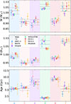 |
Fig. 2. Stellar parameters derived by the different stellar modeling methods for the six seismic solar analogs: mass (top panel), radius (middle panel), and age (bottom panel). The letters for each star are given in Table 3. The dashed lines correspond to the mean value of the different models and the dotted lines correspond to the systematics. |
Stellar fundamental parameters obtained for the six stars by the different modeling methods.
Table 3 lists the mean values and systematics (estimated as the standard deviation) of the stellar parameters for each star. The inferred masses range from ∼0.91 to 1.04 M⊙ and the radii from 0.95 to 1.08 R⊙, confirming their close similarity to the Sun despite the use of different physics and optimization techniques. The derived ages span a wide range, from ∼1.8 to 9.1 Gyr. The ensemble comparison shown in Fig. 2 indicates overall good agreement among the methods, even though the stellar evolution codes (MESA, Aarhus STellar Evolution Code (ASTEC), and Garching Stellar Evolution Code GARSTEC) adopt slightly different physics and surface-effect treatments, which may still contribute to some of the observed differences. The inferred stellar parameters (M, R, and age) are consistent within 1σ of the mean values when uncertainties are considered. Finally, none of the stars have a solar metallicity–except EPIC 212708252 (star e)–which differs from solar by several sigma.
8.1. Star-by-star seismic modeling
The star EPIC 206064678 (a) is the star closest to the Sun in terms of its mean mass of 1.016 M⊙ and radius of 0.99 R⊙, taking into account the systematics between the different methods. However, it is slightly older than the Sun, with a mean age of 5.40 Gyr. Such a star is very rare, and only a few solar twins with seismology have been studied. In comparison, the analysis of the known seismic solar twin (18 Sco) by Bazot et al. (2018) presented a bimodality in the seismic-age modeling of 4.67 and 6.95 Gyr, implying a large age uncertainty. The inferred masses and radii for this star (a) cluster fall into three groups: three models are around the mean, two are below 1σ, and the two solutions of FICO are above 1σ. They correspond to methods that use three different stellar evolution codes, which could explain the differences. All models of EPIC 206245055 (star b) have a very good agreement in all the parameters shown in Fig. 2 except for Pitchfork, but the parameters inferred with this model are still at the level of 1σ agreement.
As shown in the échelle diagram of EPIC 206371648 (star c; Fig. A.4), only five ℓ = 2 modes were fitted, with all of them having very large error bars. The ridge of these quadrupolar modes is not straight (not following the ℓ = 0 ridge). This means that the small separation of δν0, 2, which is sensitive to the properties of the core, is not well constrained. This has a direct impact on the mass and age retrieved by the best-fit model found by each method, yielding a larger discrepancy in these stellar parameters.
The inferred mass and radius of EPIC 212624487 (star d) are split into two solutions, with one favoring slightly higher mass and smaller radius and the other favoring lower mass and larger radius. Interestingly, the ages converge toward a very similar value. Together with EPIC 206064678 (star a), this star shows the smallest scatter in the age determination. EPIC 2127088252 (star e) has a very good agreement with the stellar parameters derived by the different methods. It is the oldest star of the sample, with a mean age of 9.1 Gyr.
The Kepler target KIC 3241581 (star f) shows a large dispersion in M and age, with correspondingly large uncertainties returned by the models. This likely reflects the limited seismic constraints available for this star: only eight modes are detected, with relatively large frequency uncertainties, and only a single ℓ = 2 mode. As a result, the stellar core properties are only weakly constrained. The derived stellar parameters should therefore be treated with increased caution. Indeed, when adopting the full set of modes reported by apollinaire, the modeling converges toward a significantly different solution, with a higher mass (∼1.125 M⊙), a larger radius (∼1.110 R⊙), and a younger age (∼5.07 Gyr). Interestingly, while the inferred mass and radius change noticeably, the age varies much less. This suggests that the age may not be the least well-constrained parameter for this target, similarly to what is found for star d.
8.2. Surface magnetic activity
This sample of stars is particularly interesting because, despite stellar parameters within about 10% of solar values and spanning a broader range of metallicities, all stars exhibit exceptionally low magnetic activity (see e.g., Salabert et al. 2016a; Lorenzo-Oliveira et al. 2018; Carvalho-Silva et al. 2025). While previous studies on the magnetic activity of solar-like stars showed that they had enhanced magnetic activity compared to the Sun, they mostly focused on young fast rotators (e.g., Boro Saikia et al. 2018). Recent studies have shown that the Sun exhibits a level of magnetic activity comparable to that of other solar-like stars (e.g., Reinhold et al. 2021; Mathur et al. 2023; Santos et al. 2023; Mathur et al. 2025). The magnetic activity indexes (S-index, log R′HK(B − V), and log R′IRT) computed in Sect. 5 are in a similar solar value range between minimum and maximum activity. This is not surprising as it is known that the seismic sample is biased toward stars with lower magnetic activity. Indeed, strong level of magnetic activity can be responsible for lower mode amplitude (e.g., García et al. 2010; Chaplin et al. 2011; Mathur et al. 2019; Bessila et al. 2025). To put our sample into the context of the solar twins and solar analogs studied by Lorenzo-Oliveira et al. (2018) and Carvalho-Silva et al. (2025), we converted log R′HK(B − V) to the Teff scale, log R′HK(Teff), following the prescription of Lorenzo-Oliveira et al. (2018) and using our measured S-index values. Figure 3 shows the evolution of this activity index as a function of age for different samples of stars. Our youngest star, (d), is well within the empirical relation derived by Lorenzo-Oliveira et al. (2018) for solar twins. The remaining stars that are older than the Sun are generally outside the 2σ envelope. Indeed, since our sample is not made up of solar twins but of solar analogs, they are populating the region covered by the sample of Carvalho-Silva et al. (2025), where differences could arise from the metallicities of our targets. These stars are consistent with the existence of a plateau of magnetic activity for old stars. Compared to the solar analogs from Salabert et al. (2016a), the age uncertainties are much smaller thanks to the individual-mode seismic modeling in contrast to the global seismic parameter modeling (see also Grossmann et al. 2026).
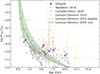 |
Fig. 3. log R′HK(Teff) as a function of age for solar twins and solar analogs. Blue squares represent the six new seismic solar analogs listed in Table 1. Orange, dark gray, and light gray circles correspond to stellar samples from the literature, as indicated in the legend. The dashed line shows the empirical relation from Lorenzo-Oliveira et al. (2018). The green shaded region represents the 2σ uncertainty envelope around this relation. The Sun is represented by the red symbol. |
It is important to note that our inferred stellar parameters have internal uncertainties larger than those of previous works on solar analogs and twins based solely on spectroscopic analysis (e.g., Lorenzo-Oliveira et al. 2018; Carvalho-Silva et al. 2025). This can be partially explained by the differential spectroscopic analysis yielding very small temperature error bars below 10 K, compared to our standard analysis providing typical values around 50 K.
8.3. Evolution of lithium
The availability of precise asteroseismic ages for this sample provides new constraints on the long-term evolution of lithium in solar analogs. As shown in Fig. 4, all six stars display lithium abundances well below the meteoritic value, with several targets providing only upper limits, despite spanning ages of ∼1.8–9.1 Gyr and a range of metallicities. This is consistent with previous seismic studies showing that substantial lithium depletion already occurs on the main sequence and continues during solar-type evolution, with a dispersion that cannot be explained by age alone (Beck et al. 2017). The binary periods exclude strong tidal angular-momentum transport (Zahn 1977, 1989), allowing the stars to be treated as effectively single. In this context, lithium depletion is likely driven by non-standard internal transport processes linked to stellar rotation and angular momentum evolution. Recent theoretical work supports this interpretation, showing that lithium evolution in solar-type stars is highly sensitive to the efficiency and depth of internal mixing and requires physics beyond standard solar-calibrated models (Charbonnel & Talon 2005; do Nascimento et al. 2009; Buldgen et al. 2025). The very low magnetic-activity levels observed in all targets indicate that surface activity alone cannot explain the depletion. In particular, EPIC 206064678–the star most similar to the Sun in terms of mass and radius–shows a lithium abundance comparable to or lower than the solar value despite being slightly older and more metal rich, supporting the conclusion that the Sun is not anomalously lithium-poor in a seismic evolutionary context. A more detailed analysis will be presented for a larger sample in future work.
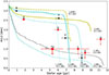 |
Fig. 4. Lithium abundance of single stars with age computed by carrying out detailed modeling with the amp code. The stars from this work are shown as red dots. Additional stars: (g) KIC 9693187 from Beck et al. (2026) and (w) KIC 10644253, (x) KIC 6116048, (y) KIC 7680114, and (z) KIC 3656476 from Beck et al. (2017) are depicted as black pentagons. Vertical, down-oriented errors indicate that the reported A(Li) is an upper limit (for stars a, c, e, f, g, and z). Toulouse–Geneva Evolution Code (TGEC) evolutionary tracks from Beck et al. (2017) are shown in cyan, and yellow represents the theoretical evolution of A(Li) for models of the indicated mass with [Fe/H] = +0.2, and −0.2 dex, respectively. The dashed black evolutionary track depicts the evolution of Li calculated by do Nascimento et al. (2009), and the solar marker depicts the measured A(Li⊙) and age of the Sun. |
In summary, using the set of stars analyzed in this work, we extended the parameter space of seismic solar analogs to encompass a wider range of metallicities and low magnetic-activity levels. Broadening this parameter space is essential for improving our understanding of the Sun’s evolution and placing it in a broader context, especially in anticipation of the PLATO mission–scheduled for launch in early 2027–which will seismically characterize thousands of solar-type stars, many of which are expected to be solar analogs spanning a wide range of parameters.
Data availability
A single table containing the individual frequencies for all the stars given in Appendix A is available at the CDS via https://cdsarc.cds.unistra.fr/viz-bin/cat/J/A+A/710/A369
Acknowledgments
This paper includes data collected by the Kepler/K2 missions. Funding for the Kepler mission is provided by the NASA Science Mission directorate. Some of the data presented in this paper were obtained from the Mikulski Archive for Space Telescopes (MAST). STScI is operated by the Association of Universities for Research in Astronomy, Inc., under NASA contract NAS5-26555. This paper also contains observations obtained with the HERMES spectrograph, which is supported by the Research Foundation – Flanders (FWO), Belgium, the Research Council of KU Leuven, Belgium, the Fonds National de la Recherche Scientifique (F.R.S.-FNRS), Belgium, the Royal Observatory of Belgium, the Observatoire de Genève, Switzerland and the Thüringer Landessternwarte Tautenburg, Germany. R.A.G., E.P., B.L., D.B.P., A.R.G.S. and V.D. acknowledge the support from the GOLF and PLATO Centre National D’Études Spatiales grants. S.M. acknowledges support by the Spanish Ministry of Science and Innovation through AEI under the Severo Ochoa Centres of Excellence Programme 2020–2023 (CEX2019-000920-S). S.N.B acknowledges support from PLATO ASI-INAF agreement n. 2015-019-R.1-2018. P.G.B. acknowledges support by the Spanish Ministry of Science and Innovation with the Ramón y Cajal fellowship number RYC-2021-033137-I and the number MRR4032204. P.G.B., D.H.G., T.M., C.A.P., D.G.R. and R.A.G. acknowledge support from the Spanish Ministry of Science and Innovation with the grant no. PID2023-146453NB-100 (PLAtoSOnG). S.M., D.G.R., D.H.G., and R.A.G. acknowledge support from the Spanish Ministry of Science and Innovation with the grant no. PID2023-149439NB-C41. D.G.R. acknowledges support from the Spanish Ministry of Science and Innovation (MICINN) with the Juan de la Cierva fellowship program under contract JDC2022-049054-I. The research of J.M. was supported by the Czech Science Foundation (GACR) project no. 24-10608O. J.B. acknowledges funding from the SNF Postdoc.Mobility grant no. P500PT_222217. GB acknowledges fundings from the Fonds National de la Recherche Scientifique (FNRS) as a postdoctoral researcher. AE received the support of a fellowship from “La Caixa” Foundation (ID 100010434) with fellowship code LCF/BQ/PI23/11970031. D.H.G. received the support of a fellowship from “la Caixa” Foundation (ID 100010434) with fellowship code is LCF/BQ/DI23/11990068. M.N.L. acknowledges support from the ESA PRODEX programme (PEA 4000142995). T.S.M. acknowledges support from NASA grant 80NSSC25K7563. Computational time at the Texas Advanced Computing Center was provided through ACCESS allocation TG-AST090107. This research was supported by the International Space Science Institute (ISSI) in Bern, through the ISSI International Team project 24-629 (“Multi-scale variability in solar and stellar magnetic cycles”) O.J.S. acknowledges the support of the Science and Technology Facilities Council (STFC). The authors wish to acknowledge the contribution of the IAC High-Performance Computing support team and hardware facilities to the results of this research. Software: ADIPLS (Christensen-Dalsgaard 2008a), AIMS code (Rendle et al. 2019), AMP (Metcalfe et al. 2009), apollinaire (Breton et al. 2022), AstroPy (Astropy Collaboration 2013, 2018), BASTA (Aguirre Børsen-Koch et al. 2022), ChatGPT (OpenAI 2023), emcee (Foreman-Mackey et al. 2013), FICO (Bétrisey et al. 2022, 2023, 2024, 2026), garstec; (Weiss & Schlattl 2008), GYRE (Townsend & Teitler 2013), Interactive Data Language (IDL; https://www.nv5geospatialsoftware.com/docs/home.html), iechelle (https://gitlab.com/dinilbose/iechelle) (Palakkatharappil, García, et al., in preparation), Matplotlib (Hunter 2007), MESA (Paxton et al. 2011, 2013, 2015), NumPy (van der Walt et al. 2011), pandas (McKinney 2010; The pandas development team 2020), PBjam (Nielsen et al. 2021, 2025), Pitchfork (Scutt et al. 2026), SciPy (Jones et al. 2001), UltraNest (Buchner 2021), yabox (Mier 2017).
References
- Abdurro’uf, Accetta, K., Aerts, C., et al. 2022, ApJS, 259, 35 [NASA ADS] [CrossRef] [Google Scholar]
- Adelberger, E. G., García, A., Robertson, R. G. H., et al. 2011, Rev. Mod. Phys., 83, 195 [Google Scholar]
- Aguirre Børsen-Koch, V., Rørsted, J. L., Justesen, A. B., et al. 2022, MNRAS, 509, 4344 [Google Scholar]
- Anderson, E. R., Duvall, T. L., Jr., & Jefferies, S. M. 1990, ApJ, 364, 699 [NASA ADS] [CrossRef] [Google Scholar]
- Andrae, R., Rix, H.-W., & Chandra, V. 2023, ApJS, 267, 8 [NASA ADS] [CrossRef] [Google Scholar]
- Angulo, C., Arnould, M., Rayet, M., et al. 1999, Nucl. Phys. A, 656, 3 [Google Scholar]
- Asplund, M., Grevesse, N., Sauval, A. J., & Scott, P. 2009, ARA&A, 47, 481 [NASA ADS] [CrossRef] [Google Scholar]
- Astropy Collaboration (Robitaille, T. P., et al.) 2013, A&A, 558, A33 [NASA ADS] [CrossRef] [EDP Sciences] [Google Scholar]
- Astropy Collaboration (Price-Whelan, A. M., et al.) 2018, AJ, 156, 123 [Google Scholar]
- Auvergne, M., Bodin, P., Boisnard, L., et al. 2009, A&A, 506, 411 [NASA ADS] [CrossRef] [EDP Sciences] [Google Scholar]
- Baglin, A., Auvergne, M., Boisnard, L., et al. 2006, COSPAR, Plenary Meet., 36, 3749 [Google Scholar]
- Ball, W. H., & Gizon, L. 2014, A&A, 568, A123 [NASA ADS] [CrossRef] [EDP Sciences] [Google Scholar]
- Ballot, J., Gizon, L., Samadi, R., et al. 2011, A&A, 530, A97 [NASA ADS] [CrossRef] [EDP Sciences] [Google Scholar]
- Barban, C., Deheuvels, S., Baudin, F., et al. 2009, A&A, 506, 51 [NASA ADS] [CrossRef] [EDP Sciences] [Google Scholar]
- Barbato, D., Ségransan, D., Udry, S., et al. 2023, A&A, 674, A114 [NASA ADS] [CrossRef] [EDP Sciences] [Google Scholar]
- Bayo, A., Rodrigo, C., Barrado Y Navascués, D., et al. 2008, A&A, 492, 277 [NASA ADS] [CrossRef] [EDP Sciences] [Google Scholar]
- Bazot, M., Campante, T. L., Chaplin, W. J., et al. 2012, A&A, 544, A106 [NASA ADS] [CrossRef] [EDP Sciences] [Google Scholar]
- Bazot, M., Creevey, O., Christensen-Dalsgaard, J., & Meléndez, J. 2018, A&A, 619, A172 [NASA ADS] [CrossRef] [EDP Sciences] [Google Scholar]
- Beck, P. G. 2026, A&A, 707, A298 [NASA ADS] [CrossRef] [EDP Sciences] [Google Scholar]
- Beck, P. G., Allende Prieto, C., Van Reeth, T., et al. 2016, A&A, 589, A27 [CrossRef] [EDP Sciences] [Google Scholar]
- Beck, P. G., do Nascimento, J. D., Jr., Duarte, T., et al. 2017, A&A, 602, A63 [NASA ADS] [CrossRef] [EDP Sciences] [Google Scholar]
- Beck, P. G., Grossmann, D. H., Steinwender, L., et al. 2024, A&A, 682, A7 [NASA ADS] [CrossRef] [EDP Sciences] [Google Scholar]
- Beck, P. G., Masseron, T., Pavlovski, K., et al. 2026, A&A, 706, L19 [NASA ADS] [CrossRef] [EDP Sciences] [Google Scholar]
- Bedding, T. R., Kjeldsen, H., Campante, T. L., et al. 2010, ApJ, 713, 935 [NASA ADS] [CrossRef] [Google Scholar]
- Berloff, G., Broomhall, A.-M., Hookway, G. T., et al. 2026, MNRAS, 546, stag092 [Google Scholar]
- Bessila, L., Deckx van Ruys, A., Buriasco, V., et al. 2025, A&A, 700, A25 [NASA ADS] [CrossRef] [EDP Sciences] [Google Scholar]
- Bétrisey, J., Pezzotti, C., Buldgen, G., et al. 2022, A&A, 659, A56 [NASA ADS] [CrossRef] [EDP Sciences] [Google Scholar]
- Bétrisey, J., Buldgen, G., Reese, D. R., et al. 2023, A&A, 676, A10 [NASA ADS] [CrossRef] [EDP Sciences] [Google Scholar]
- Bétrisey, J., Buldgen, G., Reese, D. R., & Meynet, G. 2024, A&A, 681, A99 [NASA ADS] [CrossRef] [EDP Sciences] [Google Scholar]
- Bétrisey, J., Reese, D. R., Pezzotti, C., Goupil, M., & Cunha, M. S. 2026, A&A, 710, A134 [NASA ADS] [CrossRef] [EDP Sciences] [Google Scholar]
- Böhm-Vitense, E. 1958, Z. Astrophys., 46, 108 [Google Scholar]
- Boro Saikia, S., Marvin, C. J., Jeffers, S. V., et al. 2018, A&A, 616, A108 [NASA ADS] [CrossRef] [EDP Sciences] [Google Scholar]
- Borucki, W. J., Koch, D., Jenkins, J., et al. 2009, Science, 325, 709 [Google Scholar]
- Breton, S. N., García, R. A., Ballot, J., Delsanti, V., & Salabert, D. 2022, A&A, 663, A118 [NASA ADS] [CrossRef] [EDP Sciences] [Google Scholar]
- Brown, T. M. 1984, Science, 226, 687 [Google Scholar]
- Brown, T. M., Latham, D. W., Everett, M. E., & Esquerdo, G. A. 2011, AJ, 142, 112 [Google Scholar]
- Buchner, J. 2021, J. Open Source Softw., 6, 3001 [CrossRef] [Google Scholar]
- Buder, S., Kos, J., Wang, X. E., et al. 2025, PASA, 42, e051 [Google Scholar]
- Buldgen, G., Farnir, M., Pezzotti, C., et al. 2019, A&A, 630, A126 [EDP Sciences] [Google Scholar]
- Buldgen, G., Bétrisey, J., Roxburgh, I. W., Vorontsov, S. V., & Reese, D. R. 2022, Front. Astron. Space Sci., 9, 942373 [NASA ADS] [CrossRef] [Google Scholar]
- Buldgen, G., Bétrisey, J., Pezzotti, C., Borisov, S., & Noels, A. 2025, A&A, 702, A162 [NASA ADS] [CrossRef] [EDP Sciences] [Google Scholar]
- Carvalho-Silva, G., Meléndez, J., Rathsam, A., et al. 2025, ApJ, 983, L31 [Google Scholar]
- Cayrel de Strobel, G. 1996, A&ARv, 7, 243 [CrossRef] [Google Scholar]
- Cayrel de Strobel, G., & Bentolila, C. 1989, A&A, 211, 324 [NASA ADS] [Google Scholar]
- Cayrel de Strobel, G., Knowles, N., Hernandez, G., & Bentolila, C. 1981, A&A, 94, 1 [NASA ADS] [Google Scholar]
- Chaplin, W. J., Bedding, T. R., Bonanno, A., et al. 2011, ApJ, 732, L5 [Google Scholar]
- Charbonnel, C., & Talon, S. 2005, Science, 309, 2189 [Google Scholar]
- Christensen-Dalsgaard, J. 2008a, Ap&SS, 316, 113 [Google Scholar]
- Christensen-Dalsgaard, J. 2008b, Ap&SS, 316, 13 [Google Scholar]
- Christensen-Dalsgaard, J., & Gough, D. 1984, Solar Seismology from Space (NASA), 199 [Google Scholar]
- Cox, J. P., & Giuli, R. T. 1968, Principles of Stellar Structure (Gordon and Breach) [Google Scholar]
- Creevey, O. L., Metcalfe, T. S., Schultheis, M., et al. 2017, A&A, 601, A67 [NASA ADS] [CrossRef] [EDP Sciences] [Google Scholar]
- Creevey, O. L., Sordo, R., Pailler, F., et al. 2023, A&A, 674, A26 [NASA ADS] [CrossRef] [EDP Sciences] [Google Scholar]
- Cui, X.-Q., Zhao, Y.-H., Chu, Y.-Q., et al. 2012, Res. Astron. Astrophys., 12, 1197 [Google Scholar]
- Daeppen, W., Mihalas, D., Hummer, D. G., & Mihalas, B. W. 1988, ApJ, 332, 261 [NASA ADS] [CrossRef] [Google Scholar]
- Davies, G. R., Handberg, R., Miglio, A., et al. 2014, MNRAS, 445, L94 [NASA ADS] [CrossRef] [Google Scholar]
- Davies, G. R., Chaplin, W. J., Farr, W. M., et al. 2015, MNRAS, 446, 2959 [CrossRef] [Google Scholar]
- De Silva, G. M., Freeman, K. C., Bland-Hawthorn, J., et al. 2015, MNRAS, 449, 2604 [NASA ADS] [CrossRef] [Google Scholar]
- do Nascimento, J. D., Jr., Castro, M., Meléndez, J., et al. 2009, A&A, 501, 687 [NASA ADS] [CrossRef] [EDP Sciences] [Google Scholar]
- do Nascimento, J. D., Jr., Takeda, Y., Meléndez, J., et al. 2013, ApJ, 771, L31 [Google Scholar]
- do Nascimento, J.-D., Jr., García, R. A., Mathur, S., et al. 2014, ApJ, 790, L23 [NASA ADS] [CrossRef] [Google Scholar]
- do Nascimento, J. D., Jr. , de Almeida, L., Velloso, E. N., et al. 2020, ApJ, 898, 173 [NASA ADS] [CrossRef] [Google Scholar]
- Doyle, A. P., Davies, G. R., Smalley, B., Chaplin, W. J., & Elsworth, Y. 2014, MNRAS, 444, 3592 [Google Scholar]
- Egeland, R., Soon, W., Baliunas, S., et al. 2017, ApJ, 835, 25 [NASA ADS] [CrossRef] [Google Scholar]
- Ferguson, J. W., Alexander, D. R., Allard, F., et al. 2005, ApJ, 623, 585 [Google Scholar]
- Foreman-Mackey, D., Hogg, D. W., Lang, D., & Goodman, J. 2013, PASP, 125, 306 [Google Scholar]
- Formicola, A., Imbriani, G., Costantini, H., et al. 2004, Phys. Lett. B, 591, 61 [Google Scholar]
- Gaia Collaboration (Prusti, T., et al.) 2016, A&A, 595, A1 [NASA ADS] [CrossRef] [EDP Sciences] [Google Scholar]
- Gaia Collaboration (Arenou, F., et al.) 2023a, A&A, 674, A34 [CrossRef] [EDP Sciences] [Google Scholar]
- Gaia Collaboration (Vallenari, A., et al.) 2023b, A&A, 674, A1 [NASA ADS] [CrossRef] [EDP Sciences] [Google Scholar]
- Galarza, J. Y., Lorenzo-Oliveira, D., Ferreira, T., et al. 2025, ApJ, 983, 70 [Google Scholar]
- García, R. A. 2017, EPJ Web Conf., 160, 01010 [Google Scholar]
- García, R. A., & Ballot, J. 2019, Liv. Rev. Sol. Phys., 16, 4 [Google Scholar]
- García, R. A., Mathur, S., Salabert, D., et al. 2010, Science, 329, 1032 [Google Scholar]
- García, R. A., Hekker, S., Stello, D., et al. 2011, MNRAS, 414, L6 [NASA ADS] [CrossRef] [Google Scholar]
- García, R. A., Mathur, S., Pires, S., et al. 2014, A&A, 568, A10 [Google Scholar]
- Gaulme, P., Jackiewicz, J., Appourchaux, T., & Mosser, B. 2014, ApJ, 785, 5 [NASA ADS] [CrossRef] [Google Scholar]
- Gaulme, P., Jackiewicz, J., Spada, F., et al. 2020, A&A, 639, A63 [EDP Sciences] [Google Scholar]
- Gehan, C., Godoy-Rivera, D., & Gaulme, P. 2024, A&A, 686, A93 [NASA ADS] [CrossRef] [EDP Sciences] [Google Scholar]
- Gilliland, R. L., Jenkins, J. M., Borucki, W. J., et al. 2010, ApJ, 713, L160 [Google Scholar]
- Gilmore, G., Randich, S., Asplund, M., et al. 2012, Messenger, 147, 25 [Google Scholar]
- Godoy-Rivera, D., Mathur, S., García, R. A., et al. 2025, A&A, 696, A243 [Google Scholar]
- Godoy-Rivera, D., Grossmann, D. H., Richey-Yowell, T., et al. 2026a, RNAAS, submitted [Google Scholar]
- Godoy-Rivera, D., Mathur, S., Richey-Yowell, T., et al. 2026b, A&A, submitted [Google Scholar]
- González-Cuesta, L., Mathur, S., García, R. A., et al. 2023, A&A, 674, A106 [NASA ADS] [CrossRef] [EDP Sciences] [Google Scholar]
- Grevesse, N., & Sauval, A. J. 1998, Space Sci. Rev., 85, 161 [Google Scholar]
- Grossmann, D. H., Beck, P. G., Mathur, S., et al. 2025, A&A, 696, A42 [NASA ADS] [CrossRef] [EDP Sciences] [Google Scholar]
- Grossmann, D. H., Mathur, S., Beck, P. G., et al. 2026, A&A, submitted [Google Scholar]
- Gustafsson, B., Edvardsson, B., Eriksson, K., et al. 2008, A&A, 486, 951 [NASA ADS] [CrossRef] [EDP Sciences] [Google Scholar]
- Hammer, J. W., Fey, M., Kunz, R., et al. 2005, Nucl. Phys. A, 758, 363 [NASA ADS] [CrossRef] [Google Scholar]
- Hardorp, J. 1978, A&A, 63, 383 [NASA ADS] [Google Scholar]
- Harvey, J. 1985, ESA SP, 235, 199 [Google Scholar]
- Hayes, C. R., Masseron, T., Sobeck, J., et al. 2022, ApJS, 262, 34 [NASA ADS] [CrossRef] [Google Scholar]
- Heiter, U., Lind, K., Bergemann, M., et al. 2021, A&A, 645, A106 [EDP Sciences] [Google Scholar]
- Hookway, G. T., Nielsen, M. B., Davies, G. R., et al. 2025, MNRAS, 544, 3247 [Google Scholar]
- Horch, E. P., Falta, D., Anderson, L. M., et al. 2010, AJ, 139, 205 [Google Scholar]
- Hourihane, A., François, P., Worley, C. C., et al. 2023, A&A, 676, A129 [NASA ADS] [CrossRef] [EDP Sciences] [Google Scholar]
- Howell, S. B., Sobeck, C., Haas, M., et al. 2014, PASP, 126, 398 [Google Scholar]
- Huber, D., Bryson, S. T., Haas, M. R., et al. 2016, ApJS, 224, 2 [Google Scholar]
- Huber, D., White, T. R., Metcalfe, T. S., et al. 2022, AJ, 163, 79 [NASA ADS] [CrossRef] [Google Scholar]
- Hummer, D. G., & Mihalas, D. 1988, ApJ, 331, 794 [NASA ADS] [CrossRef] [Google Scholar]
- Hunter, J. D. 2007, Comput. Sci. Eng., 9, 90 [NASA ADS] [CrossRef] [Google Scholar]
- Iglesias, C. A., & Rogers, F. J. 1996, ApJ, 464, 943 [NASA ADS] [CrossRef] [Google Scholar]
- Irwin, A. W. 2012, Astrophysics Source Code Library [record ascl:1211.002] [Google Scholar]
- Jermyn, A. S., Bauer, E. B., Schwab, J., et al. 2023, ApJS, 265, 15 [NASA ADS] [CrossRef] [Google Scholar]
- Jones, E., Oliphant, T., Peterson, P., et al. 2001, SciPy: Open Source Scientific Tools for Python [Google Scholar]
- Karoff, C., Metcalfe, T. S., Santos, Â. R. G., et al. 2018, ApJ, 852, 46 [Google Scholar]
- Kervella, P., Arenou, F., Mignard, F., & Thévenin, F. 2019, A&A, 623, A72 [NASA ADS] [CrossRef] [EDP Sciences] [Google Scholar]
- Kippenhahn, R., Weigert, A., & Weiss, A. 2013, Stellar Structure and Evolution (Berlin: Springer) [Google Scholar]
- Kjeldsen, H., Bedding, T. R., & Christensen-Dalsgaard, J. 2008, ApJ, 683, L175 [Google Scholar]
- Lada, C. J. 2006, ApJ, 640, L63 [Google Scholar]
- Lanzafame, A. C., Brugaletta, E., Frémat, Y., et al. 2023, A&A, 674, A30 [NASA ADS] [CrossRef] [EDP Sciences] [Google Scholar]
- Lebreton, Y., & Goupil, M. J. 2014, A&A, 569, A21 [NASA ADS] [CrossRef] [EDP Sciences] [Google Scholar]
- Li, T., Davies, G. R., Nielsen, M., Cunha, M. S., & Lyttle, A. J. 2023, MNRAS, 523, 80 [Google Scholar]
- Lindegren, L., Klioner, S. A., Hernández, J., et al. 2021, A&A, 649, A2 [EDP Sciences] [Google Scholar]
- Lindsay, C. J., Hon, M., Ong, J. M. J., et al. 2025, ApJ, 989, 189 [Google Scholar]
- Lorenzo-Oliveira, D., Freitas, F. C., Meléndez, J., et al. 2018, A&A, 619, A73 [NASA ADS] [CrossRef] [EDP Sciences] [Google Scholar]
- Luger, R., Agol, E., Kruse, E., et al. 2016, AJ, 152, 100 [Google Scholar]
- Luger, R., Kruse, E., Foreman-Mackey, D., Agol, E., & Saunders, N. 2018, AJ, 156, 99 [Google Scholar]
- Lund, M. N., Silva Aguirre, V., Davies, G. R., et al. 2017, ApJ, 835, 172 [Google Scholar]
- Lund, M. N., Basu, S., Bieryla, A., et al. 2024, A&A, 688, A13 [NASA ADS] [CrossRef] [EDP Sciences] [Google Scholar]
- Lyttle, A. J., Davies, G. R., Li, T., et al. 2021, MNRAS, 505, 2427 [NASA ADS] [CrossRef] [Google Scholar]
- Majewski, S. R., Schiavon, R. P., Frinchaboy, P. M., et al. 2017, AJ, 154, 94 [NASA ADS] [CrossRef] [Google Scholar]
- Mamajek, E. E., & Hillenbrand, L. A. 2008, ApJ, 687, 1264 [Google Scholar]
- Mamajek, E. E., Torres, G., Prsa, A., et al. 2015, ArXiv e-prints [arXiv:1510.06262] [Google Scholar]
- Masseron, T., Merle, T., & Hawkins, K. 2016, Astrophysics Source Code Library [record ascl:1605.004] [Google Scholar]
- Mathur, S., García, R. A., Régulo, C., et al. 2010, A&A, 511, A46 [NASA ADS] [CrossRef] [EDP Sciences] [Google Scholar]
- Mathur, S., García, R. A., Bugnet, L., et al. 2019, Front. Astron. Space Sci., 6, 46 [Google Scholar]
- Mathur, S., García, R. A., Breton, S., et al. 2022, A&A, 657, A31 [NASA ADS] [CrossRef] [EDP Sciences] [Google Scholar]
- Mathur, S., Claytor, Z. R., Santos, Â. R. G., et al. 2023, ApJ, 952, 131 [NASA ADS] [CrossRef] [Google Scholar]
- Mathur, S., Santos, Â. R. G., Claytor, Z. R., et al. 2025, ApJ, 982, 114 [Google Scholar]
- McKinney, W. 2010, in Proceedings of the 9th Python in Science Conference (SciPy), 56 [Google Scholar]
- Metcalfe, T. S., & Charbonneau, P. 2003, J. Comput. Phys., 185, 176 [NASA ADS] [CrossRef] [Google Scholar]
- Metcalfe, T. S., Creevey, O. L., & Christensen-Dalsgaard, J. 2009, ApJ, 699, 373 [Google Scholar]
- Metcalfe, T. S., Chaplin, W. J., Appourchaux, T., et al. 2012, ApJ, 748, L10 [Google Scholar]
- Metcalfe, T. S., Egeland, R., & van Saders, J. 2016, ApJ, 826, L2 [Google Scholar]
- Metcalfe, T. S., Finley, A. J., Kochukhov, O., et al. 2022, ApJ, 933, L17 [NASA ADS] [CrossRef] [Google Scholar]
- Michaud, G., & Proffitt, C. R. 1993, ASP Conf. Ser., 40, 246 [Google Scholar]
- Mier, P. R. 2017, https://doi.org/10.5281/zenodo.848679 [Google Scholar]
- Mihalas, D., Dappen, W., & Hummer, D. G. 1988, ApJ, 331, 815 [NASA ADS] [CrossRef] [Google Scholar]
- Mihalas, D., Hummer, D. G., Mihalas, B. W., & Daeppen, W. 1990, ApJ, 350, 300 [NASA ADS] [CrossRef] [Google Scholar]
- Moe, M., & Di Stefano, R. 2017, ApJS, 230, 15 [Google Scholar]
- Nielsen, M. B., Davies, G. R., Ball, W. H., et al. 2021, AJ, 161, 62 [NASA ADS] [CrossRef] [Google Scholar]
- Nielsen, M. B., Ong, J. M. J., Hatt, E. J., et al. 2025, AJ, 169, 322 [Google Scholar]
- OpenAI. 2023, arXiv e-prints [arXiv:2303.08774] [Google Scholar]
- Otí Floranes, H., Christensen-Dalsgaard, J., & Thompson, M. J. 2005, MNRAS, 356, 671 [CrossRef] [Google Scholar]
- Paquette, C., Pelletier, C., Fontaine, G., & Michaud, G. 1986, ApJS, 61, 177 [Google Scholar]
- Paxton, B., Bildsten, L., Dotter, A., et al. 2011, ApJS, 192, 3 [Google Scholar]
- Paxton, B., Cantiello, M., Arras, P., et al. 2013, ApJS, 208, 4 [Google Scholar]
- Paxton, B., Marchant, P., Schwab, J., et al. 2015, ApJS, 220, 15 [Google Scholar]
- Paxton, B., Schwab, J., Bauer, E. B., et al. 2018, ApJS, 234, 34 [NASA ADS] [CrossRef] [Google Scholar]
- Paxton, B., Smolec, R., Schwab, J., et al. 2019, ApJS, 243, 10 [Google Scholar]
- Penoyre, Z., Belokurov, V., & Evans, N. W. 2022, MNRAS, 513, 2437 [NASA ADS] [CrossRef] [Google Scholar]
- Pérez Hernández, F., García, R. A., Mathur, S., Santos, Â. R. G., & Régulo, C. 2019, Front. Astron. Space Sci., 6, 41 [CrossRef] [Google Scholar]
- Pires, S., Mathur, S., García, R. A., et al. 2015, A&A, 574, A18 [NASA ADS] [CrossRef] [EDP Sciences] [Google Scholar]
- Pourbaix, D., Tokovinin, A. A., Batten, A. H., et al. 2004, A&A, 424, 727 [NASA ADS] [CrossRef] [EDP Sciences] [Google Scholar]
- Randich, S., Gilmore, G., & Gaia-ESO Consortium. 2013, Messenger, 154, 47 [NASA ADS] [Google Scholar]
- Raskin, G., van Winckel, H., Hensberge, H., et al. 2011, A&A, 526, A69 [CrossRef] [EDP Sciences] [Google Scholar]
- Rauer, H., Catala, C., Aerts, C., et al. 2014, Exp. Astron., 38, 249 [Google Scholar]
- Rauer, H., Aerts, C., Cabrera, J., et al. 2025, Exp. Astron., 59, 26 [Google Scholar]
- Recio-Blanco, A., de Laverny, P., Palicio, P. A., et al. 2023, A&A, 674, A29 [NASA ADS] [CrossRef] [EDP Sciences] [Google Scholar]
- Reese, D. R., Marques, J. P., Goupil, M. J., Thompson, M. J., & Deheuvels, S. 2012, A&A, 539, A63 [NASA ADS] [CrossRef] [EDP Sciences] [Google Scholar]
- Reinhold, T., Shapiro, A. I., Witzke, V., et al. 2021, ApJ, 908, L21 [NASA ADS] [CrossRef] [Google Scholar]
- Rendle, B. M., Buldgen, G., Miglio, A., et al. 2019, MNRAS, 484, 771 [Google Scholar]
- Ricker, G. R., Winn, J. N., Vanderspek, R., et al. 2014, SPIE Conf. Ser., 9143, 20 [Google Scholar]
- Rogers, F. J., & Iglesias, C. A. 1992, ApJS, 79, 507 [CrossRef] [Google Scholar]
- Rogers, F. J., & Nayfonov, A. 2002, ApJ, 576, 1064 [Google Scholar]
- Rogers, F. J., Swenson, F. J., & Iglesias, C. A. 1996, ApJ, 456, 902 [Google Scholar]
- Roxburgh, I. W., & Vorontsov, S. V. 2003, A&A, 411, 215 [NASA ADS] [CrossRef] [EDP Sciences] [Google Scholar]
- Salabert, D., García, R. A., Beck, P. G., et al. 2016a, A&A, 596, A31 [NASA ADS] [CrossRef] [EDP Sciences] [Google Scholar]
- Salabert, D., Régulo, C., García, R. A., et al. 2016b, A&A, 589, A118 [CrossRef] [EDP Sciences] [Google Scholar]
- Salpeter, E. E. 1955, ApJ, 121, 161 [Google Scholar]
- Santos, Â. R. G., Mathur, S., García, R. A., et al. 2023, A&A, 672, A56 [NASA ADS] [CrossRef] [EDP Sciences] [Google Scholar]
- Scutt, O. J., Davies, G. R., Stokholm, A., et al. 2026, MNRAS, stag018 [Google Scholar]
- Sobol, I. 1977, USSR Comput. Math. Math. Phys., 16, 236 [Google Scholar]
- Sobol, I., & Levithan, Y. 1976, IPM Akademii Nauk SSSR [Google Scholar]
- Speagle, J. S. 2020, MNRAS, 493, 3132 [Google Scholar]
- Suárez Mascareño, A., Rebolo, R., González Hernández, J. I., & Esposito, M. 2015, MNRAS, 452, 2745 [Google Scholar]
- The pandas development team. 2020, https://doi.org/10.5281/zenodo.3509134 [Google Scholar]
- Thoul, A. A., Bahcall, J. N., & Loeb, A. 1994, ApJ, 421, 828 [Google Scholar]
- Tokovinin, A. 2018, AJ, 156, 48 [Google Scholar]
- Tokovinin, A., Mason, B. D., Mendez, R. A., Costa, E., & Horch, E. P. 2020, AJ, 160, 7 [NASA ADS] [CrossRef] [Google Scholar]
- Townsend, R. H. D., & Teitler, S. A. 2013, MNRAS, 435, 3406 [Google Scholar]
- van der Walt, S., Colbert, S. C., & Varoquaux, G. 2011, CiSE, 13, 22 [Google Scholar]
- Vernazza, J. E., Avrett, E. H., & Loeser, R. 1981, ApJS, 45, 635 [Google Scholar]
- Videla, M., Mendez, R. A., Clavería, R. M., Silva, J. F., & Orchard, M. E. 2022, AJ, 163, 220 [NASA ADS] [CrossRef] [Google Scholar]
- Weiss, A., & Schlattl, H. 2008, Ap&SS, 316, 99 [CrossRef] [Google Scholar]
- Yana Galarza, J., López-Valdivia, R., Lorenzo-Oliveira, D., et al. 2021, MNRAS, 504, 1873 [NASA ADS] [CrossRef] [Google Scholar]
- Zahn, J.-P. 1977, A&A, 57, 383 [NASA ADS] [Google Scholar]
- Zahn, J.-P. 1989, A&A, 220, 112 [NASA ADS] [Google Scholar]
- Zhao, G., Zhao, Y.-H., Chu, Y.-Q., Jing, Y.-P., & Deng, L.-C. 2012, Res. Astron. Astrophys., 12, 723 [NASA ADS] [CrossRef] [Google Scholar]
- Zheng, Z., Cao, Z., Deng, H., et al. 2023, ApJS, 266, 18 [Google Scholar]
- Zong, W., Fu, J.-N., De Cat, P., et al. 2020, ApJS, 251, 15 [NASA ADS] [CrossRef] [Google Scholar]
These data products are known as KEPSEISMIC and are available on MAST: http://dx.doi.org/10.17909/t9-mrpw-gc07
Note that, for the purposes of this comparison and Fig. 1, we take [Fe/H] as [M/H] and compare both of them directly.
Appendix A: Summary of the p-mode frequencies
A.1. KIC 3241581
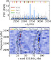 |
Fig. A.1. Left panel: PSD of KIC 3241581 in the region of the oscillation power excess. The full excess is shown in S/N units, with the original PSD in black and its smoothed version (using a 10-point window) in grey. The blue curve represents the combined model based on the frequencies extracted by apollinaire, which are marked by vertical dashes: red for ℓ = 0, yellow for ℓ = 1, and green for ℓ = 2. Right panel: Corresponding échelle diagram. Observed mode frequencies are shown as filled symbols where darker ones indicate the frequencies included in the model, while lighter ones were excluded. Color coding is consistent with the left panel: red circles, yellow diamonds, and green triangles represent ℓ = 0, ℓ = 1, and ℓ = 2, respectively. Model frequencies are plotted as open black symbols with consistent markers. This figure was produced using the Python module pareidolia (available at https://gitlab.com/evapanetier/pareidolia.git), which is designed for seismic data analysis. |
Frequencies and associated incertitude for each detected modes (n, l), and depending on the peakbagging code, for KIC 3241581.
A.2. EPIC 206064678
Same as Table A.1 but for EPIC 206064678.
A.3. EPIC 206245055
Same as Table A.1 but for EPIC 206245055.
A.4. EPIC 206371648
Same as Table A.1 but for EPIC 206371648.
A.5. EPIC 212624487
Same as Table A.1 but for EPIC 212624487.
A.4. EPIC 212708252
Same as Table A.1 but for EPIC 212708252.
Appendix B: Radial velocity analysis of KIC 3241581
KIC 3241581 was reported to be a binary by Beck et al. (2016) and has been continuously monitored for more than six years with the same instrumentation. We fitted a Keplerian orbit to the 40 available RV measurements, obtaining a period of 1316.4 ± 1.0 days and a moderate eccentricity of 0.367 ± 0.002. The full set of orbital parameters is listed in Table B.1. The RV time series together with the best-fit model and the corresponding residuals are shown in Fig. B.1.
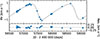 |
Fig. B.1. Spectroscopic observations and orbital model of KIC 3241581 from the Mercator/HERMES data (top panel), with the residuals shown in the bottom panel. |
Orbital elements of KIC 3241581.
The peak-to-peak RV amplitude of ∼2 km s−1 is relatively small compared to samples of other main-sequence binaries (e.g., Beck et al. 2017; Beck 2026). The combination of a high RUWE value (∼6) and small RV variations suggests that the orientation of the system may be close to plane-on.
All Tables
Photometric, RV, and astrometric information of the six candidate solar analogs.
Stellar fundamental parameters obtained for the six stars by the different modeling methods.
Frequencies and associated incertitude for each detected modes (n, l), and depending on the peakbagging code, for KIC 3241581.
All Figures
|
Fig. 1. Comparison of atmospheric parameters: HERMES versus spectroscopic surveys. The top, middle, and bottom panels show the comparison of effective temperatures, surface gravities, and metallicities. The HERMES values are on the x-axis, and the spectroscopic surveys are on the y-axis, with Andrae et al. (2023) in red, APOGEE DR17 in blue, and Gaia DR3gspspec in green. Each target is shown by a different symbol, as indicated in the middle panel legend. The Andrae et al. (2023) values show the better overall agreement, and largest overlap, with HERMES. |
| In the text | |
|
Fig. 2. Stellar parameters derived by the different stellar modeling methods for the six seismic solar analogs: mass (top panel), radius (middle panel), and age (bottom panel). The letters for each star are given in Table 3. The dashed lines correspond to the mean value of the different models and the dotted lines correspond to the systematics. |
| In the text | |
|
Fig. 3. log R′HK(Teff) as a function of age for solar twins and solar analogs. Blue squares represent the six new seismic solar analogs listed in Table 1. Orange, dark gray, and light gray circles correspond to stellar samples from the literature, as indicated in the legend. The dashed line shows the empirical relation from Lorenzo-Oliveira et al. (2018). The green shaded region represents the 2σ uncertainty envelope around this relation. The Sun is represented by the red symbol. |
| In the text | |
|
Fig. 4. Lithium abundance of single stars with age computed by carrying out detailed modeling with the amp code. The stars from this work are shown as red dots. Additional stars: (g) KIC 9693187 from Beck et al. (2026) and (w) KIC 10644253, (x) KIC 6116048, (y) KIC 7680114, and (z) KIC 3656476 from Beck et al. (2017) are depicted as black pentagons. Vertical, down-oriented errors indicate that the reported A(Li) is an upper limit (for stars a, c, e, f, g, and z). Toulouse–Geneva Evolution Code (TGEC) evolutionary tracks from Beck et al. (2017) are shown in cyan, and yellow represents the theoretical evolution of A(Li) for models of the indicated mass with [Fe/H] = +0.2, and −0.2 dex, respectively. The dashed black evolutionary track depicts the evolution of Li calculated by do Nascimento et al. (2009), and the solar marker depicts the measured A(Li⊙) and age of the Sun. |
| In the text | |
|
Fig. A.1. Left panel: PSD of KIC 3241581 in the region of the oscillation power excess. The full excess is shown in S/N units, with the original PSD in black and its smoothed version (using a 10-point window) in grey. The blue curve represents the combined model based on the frequencies extracted by apollinaire, which are marked by vertical dashes: red for ℓ = 0, yellow for ℓ = 1, and green for ℓ = 2. Right panel: Corresponding échelle diagram. Observed mode frequencies are shown as filled symbols where darker ones indicate the frequencies included in the model, while lighter ones were excluded. Color coding is consistent with the left panel: red circles, yellow diamonds, and green triangles represent ℓ = 0, ℓ = 1, and ℓ = 2, respectively. Model frequencies are plotted as open black symbols with consistent markers. This figure was produced using the Python module pareidolia (available at https://gitlab.com/evapanetier/pareidolia.git), which is designed for seismic data analysis. |
| In the text | |
 |
Fig. A.2. Same as Fig. A.1 but for EPIC 206064678. |
| In the text | |
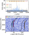 |
Fig. A.3. Same as Fig. A.1 but for EPIC 206245055. |
| In the text | |
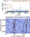 |
Fig. A.4. Same as Fig. A.1 but for EPIC 206371648. |
| In the text | |
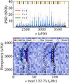 |
Fig. A.5. Same as Fig. A.1 but for EPIC 212624487. |
| In the text | |
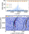 |
Fig. A.6. Same as Fig. A.1 but for EPIC 212708252. |
| In the text | |
|
Fig. B.1. Spectroscopic observations and orbital model of KIC 3241581 from the Mercator/HERMES data (top panel), with the residuals shown in the bottom panel. |
| In the text | |
Current usage metrics show cumulative count of Article Views (full-text article views including HTML views, PDF and ePub downloads, according to the available data) and Abstracts Views on Vision4Press platform.
Data correspond to usage on the plateform after 2015. The current usage metrics is available 48-96 hours after online publication and is updated daily on week days.
Initial download of the metrics may take a while.