


| Issue |
A&A
Volume 711, July 2026
|
|
|---|---|---|
| Article Number | A216 | |
| Number of page(s) | 13 | |
| Section | The Sun and the Heliosphere | |
| DOI | https://doi.org/10.1051/0004-6361/202659279 | |
| Published online | 16 July 2026 | |
Mg II h&k spectral line properties computed using 3D radiative transfer in an enhanced network region simulated with the MURaM-ChE code
1
Max-Planck-Institut für Sonnensystemforschung, Justus-von-Liebig-Weg 3, 37077 Göttingen, Germany
2
Institute for Solar Physics, Department of Astronomy, Stockholm University, AlbaNova University Centre, 106 91 Stockholm, Sweden
★ Corresponding author: This email address is being protected from spambots. You need JavaScript enabled to view it.
Received:
2
February
2026
Accepted:
14
May
2026
Abstract
Context. Synthetic spectral lines from radiative magnetohydrodynamic models are essential in order to interpret the observations of the solar chromosphere, but only a few computations in the literature take 3D effects in the synthesis into account. The Mg II h&k lines form in the middle to upper chromosphere and are well suited to studying the structure of the chromosphere. However, the details of their formation in the solar chromosphere are not fully understood.
Aims. We studied the effects of 3D radiative transfer (RT) on the Mg II h&k line properties and tested the known correlations between the underlying atmosphere and spectral line features in a new model of the chromosphere.
Methods. We forward modeled the Mg II h&k lines in 3D RT with partial frequency redistribution (PRD) in a self-consistent 3D radiative magnetohydrodynamic (rMHD) simulation with non-local thermodynamic equilibrium (NLTE) energy transport and non-equilibrium (NE) hydrogen ionization of an enhanced network (EN) region simulated with the chromospheric extension of MURaM (MURaM-ChE). We compared the spectra computed with 3D RT to those computed with 1.5D RT and to observations from the Interface Region Imaging Spectrograph (IRIS). Furthermore, we tested the correlations between the spectral line properties and underlying atmospheric properties such as temperature and velocity structure.
Results. The spatially averaged Mg II h&k spectral lines computed with 3D RT match approximately a typical IRIS observation, which includes quiet sun and network elements. However, the peak separation is still slightly lower in the simulation. In contrast, the 1.5D RT spectra tend to overestimate the peak intensities and the central minimum significantly. In the MURaM-ChE model, the qualitative difference between 1.5D and 3D RT results is even more pronounced than in the public Bifrost snapshot, as given in the literature. We found that this large discrepancy might be partly attributed to the horizontal velocities that are naturally included in the full 3D RT synthesis, but not in typical 1.5D RT computations. We confirmed that the correlations between spectral line properties and the underlying atmosphere from the MURaM-ChE simulation are similar to those obtained from Bifrost, but show more scatter due to the more dynamic atmosphere. In addition to already known correlations, we found that the k2v (blue) peak of the Mg II k line forms preferably in upflows, whereas the k2r (red) peak forms preferably in downflows.
Conclusions. The Mg II h&k lines computed with 3D RT match the observations better in the core intensities and their distribution on the Sun compared to 1.5D computations. This underlines the importance of 3D RT in the forward modeling of Mg II h&k.
Key words: radiative transfer / Sun: atmosphere / Sun: chromosphere
© The Authors 2026
 Open Access article, published by EDP Sciences, under the terms of the Creative Commons Attribution License (https://creativecommons.org/licenses/by/4.0), which permits unrestricted use, distribution, and reproduction in any medium, provided the original work is properly cited.
This article is published in open access under the Subscribe to Open model.
Open access funding provided by Max Planck Society.
1. Introduction
The solar chromosphere is an interface between the underlying photosphere and the corona above. The causes of many phenomena, such as the heating of the chromosphere (e.g., Withbroe & Noyes 1977) or the strong dynamics it displays, are not understood. Additionally, the evolution of fine structures such as spicules, their interaction with the magnetic field, and their role in supplying mass and energy to the corona are under debate (Carlsson et al. 2019). The inference of physical quantities such as temperature, velocity, density, and magnetic field is limited through a few strong spectral lines forming in the chromosphere. Because of the decreasing density with height, spectral line formation in the chromosphere is subject to non-LTE (NLTE) conditions. In addition, some strong resonance lines such as Ca II H & K and Mg II h&k show partial frequency redistribution (PRD) effects through scattering (e.g., Milkey & Mihalas 1974). Furthermore, already in the 1980s it became clear from Lyman α observations that the chromosphere is inhomogeneous and plane-parallel modeling is only a zeroth-order approximation (e.g., Bonnet et al. 1980). Only recently has it become possible to model chromospheric lines including both a 3D model atmosphere and 3D RT. Examples are the Ca IIλ854.2 nm line (Leenaarts et al. 2009), Hα (Leenaarts et al. 2012), Mg II h&k (Leenaarts et al. 2013a) and (with a PRD treatment, Sukhorukov & Leenaarts 2017), and Ca II H & K (Bjørgen et al. 2018). An alternative to the computationally expensive 3D RT calculations is 1.5D RT. In this approximation the spectral lines are synthesized from a 3D atmosphere model, but each vertical column is treated as an independent plane-parallel atmosphere.
Two main strategies are used to interpret the observations. Inversions aim to reconstruct an atmosphere model to fit an observed spectral line profile. However, the model atmospheres are kept relatively simple, and the solution is not always unique. In other words, different model atmospheres may lead to very similar spectral line shapes (for reviews of inversions see e.g., del Toro Iniesta & Ruiz Cobo 2016; de la Cruz Rodríguez & van Noort 2017). In addition, fudge parameters such as microturbulence are introduced to fit the observed line widths, while the actual velocity structure remains unresolved. Inversion codes solve the RT problem, but they are generally restricted to 1.5D RT as their calculations can easily become expensive, although approaches to take 3D RT effects in inversions into account exist (Štěpán et al. 2022).
The other main strategy is based on forward modeling. In the first step, a model of the solar atmosphere is simulated. In the second step, detailed RT computations are conducted post-processing. In contrast to inversions, forward modeling does not aim to exactly reproduce a single observation. However, the advantage is that through the knowledge of all quantities in the atmosphere, line formation can be studied in detail. By comparing the atmosphere with the resulting spectra, possible correlations can be identified, which can be used to interpret observations without performing inversions.
In this paper, we focus on the Mg II h&k lines. A typical line profile of Mg II k observed in the quiet Sun (QS) shows a double-reversed line core. The inner wings, which are the minimum intensities before the first reversal, are called k1v and k1r, where “v” indicates the blue or violet part of the spectrum with respect to the rest wavelength and “r” indicates the red part. The peaks are similarly labeled k2v and k2r. The central reversal is called k3. The Mg II h line shows properties similar to Mg II k and has therefore analogous labeling. These spectral features form at different atmospheric heights (see, e.g., Vernazza et al. 1981, Fig. 1), and are thus sensitive to local conditions. The k1 features form in the low chromosphere close to the temperature minimum in a plane-parallel atmosphere. The k2 peaks form in the mid chromosphere and the k3 minimum just below the transition region.
Recent studies of the Mg II h&k line formation were presented by Avrett et al. (2013) for different regions on the sun using 1D model atmospheres. The authors investigated the center-to-limb variation (CLV) and the effect of the upflows and downflows on the resulting Mg II k line profiles. Leenaarts et al. (2013a,b) and Pereira et al. (2013) used a snapshot of a 3D EN simulation (Carlsson et al. 2016, herafter public Bifrost snapshot) computed with the Bifrost code (Gudiksen et al. 2011). There it was found, for example, that the Doppler shifts of the k3 and h3 features are good indicators of the vertical velocity in the upper chromosphere, while the differences between the k3 and h3 Doppler shifts correlate with the velocity gradients in the upper chromosphere. The k2 and h2 peak intensities can be used to estimate the temperature in the middle chromosphere, while the peak intensity ratios of the k2 or h2 peaks correlate with up- or downflows in the upper chromosphere. A summary of these diagnostics can be found in Pereira et al. (2013, Table 4). These correlations have been proven useful, among other studies, to interpret variability of Mg II h in full disk mosaics by Schmit et al. (2015), to constrain chromospheric dynamics by Gošić et al. (2018) and Hannah et al. (2019), and to study the velocity structure of prominences by (e.g., Peat et al. 2021). A phenomenon of the Mg II h&k line formation that has so far not been entirely understood is the difference in the emergent intensity between the quiet Sun (qs) and coronal holes (Kayshap et al. 2018).
The computations of Leenaarts et al. (2013b) and Pereira et al. (2013) resulted in Mg II h&k profiles with too narrow line widths and too weak peak intensities when compared to observations. The above-mentioned authors and Carlsson et al. (2016) argued that a higher numerical resolution in the simulation might help to resolve more dynamics and reduce such discrepancies. The simulations of Martínez-Sykora et al. (2023) showed a better match with observed profiles by using a high horizontal resolution of 5 km. The flux emergence simulations of Hansteen et al. (2023) also show a good match with observations, even though the spatial resolution of 100 km is relatively low. This suggests that higher mass loading of the chromosphere is required to reproduce the observed line width. Recently, Ondratschek et al. (2024), hereafter Pub I, presented a relatively close match of the Mg II h&k lines from an EN simulation with observations of the QS. The simulation they used was computed with the recently developed MURaM-ChE1 code (Przybylski et al. 2022). While the resolution in the MURaM-ChE model was relatively moderate, i.e., 20 km vertically and 23.4 km horizontally, in Pub I it was found that the MURaM-ChE atmosphere is more dynamic than the public Bifrost snapshot, thus explaining the improved match.
The authors also found that the Mg II h&k peak intensities are larger and the line width slightly smaller in the spatially averaged simulated profiles than in the observations. In Pub I the Mg II h&k spectra were computed in the 1.5D RT approximation where each column in the atmosphere is treated as an independent plane-parallel atmosphere.
For this work, we extended these studies by computing the spectra of the same simulation snapshot, but in 3D RT by using the Multi3D code (Leenaarts et al. 2009). Our goal was to study the impact of 3D RT for the Mg II h&k lines in the MURaM-ChE model, which was shown to be important by Sukhorukov & Leenaarts (2017), Bjørgen et al. (2019), and Judge et al. (2020). In addition, we tested the robustness of the correlations found by Leenaarts et al. (2013b) and Pereira et al. (2013) in the MURaM-ChE simulation used here.
This paper is structured as follows. In Sect. 2 we briefly describe the MURaM-ChE model, the RT computations, and the observation we used for comparison. In Sect. 3 we describe our results, and in Sect. 4 we provide a summary and discussion. In Sect. 5 we present our conclusions.
2. Methods
In the following, we describe the MURaM-ChE EN simulation and the Multi3D code, which we used to compute the Mg II h&k spectra in 1.5D RT and 3D RT. We then describe how the spectra were degraded to the instrumental conditions of the Interface Region Imaging Spectrometer (IRIS). After this, we describe the observation to which we compare our results.
2.1. The MURaM-ChE model
We use the same model atmosphere as described in Pub I, which represents an EN region with a large-scale bipolar structure. This model was designed to be similar to the public Bifrost snapshot (Carlsson et al. 2016), including the same large-scale field geometry. The model is simulated with the chromospheric extension of the MURaM radiaton-MHD (rMHD) code (Przybylski et al. 2022), which includes NLTE line losses and a nonequilibrium (NE) treatment of hydrogen ionization. The model atmosphere extends over a solar volume of 24 Mm × 24 Mm × 24 Mm with a horizontal resolution of 23.4 km and a vertical resolution of 20 km. The EN simulation is based on the small-scale dynamo (SSD) simulation by Przybylski et al. (2025). The convection zone extends roughly from z = −7 Mm to z = 0 Mm, where z = 0 Mm lies at the average τ500 = 1 height. The atmosphere extends up to z = 17 Mm. We refer to Pub I for more details.
2.2. The Multi3D code
To compute the spectra of Mg II h&k in 3D RT we utilize the Multi3D code (Leenaarts & Carlsson 2009) with the extension to compute PRD spectra (Sukhorukov & Leenaarts 2017). In Multi3D, the radiative transfer equation (RTE) and the equations of statistical equilibrium (SE) are solved simultaneously. The solution is computed iteratively based on the multilevel accelerated Λ-iteration (MALI) scheme with preconditioned radiative rates according to (Rybicki & Hummer 1991, 1992) until convergence of relative population changes with a tolerance of 10−3 is reached. The RTE is integrated by using the short characteristics scheme. This allows for domain decomposition and a parallel treatment of the problem. The angular quadrature follows the 24-angle A4 set of Carlson (1963). We compute the Mg II h&k lines by using the 4+1 level model atom similar to Sukhorukov & Leenaarts (2017) and Bjørgen et al. (2019). The model atom is described in Leenaarts et al. (2013a). This is a compromise between accuracy and computational time. As demonstrated by Leenaarts et al. (2013a) the 4+1 level shows only small deviations from the more accurate 10+1 level atom and is therefore a good choice for expensive 3D RT computations. We used only every other column from the 3D MHD cubes to speed up the computation. This effectively reduces the horizontal resolution to ≈48 km. Multi3D has the option to compute spectra also in the 1.5D RT plane-parallel mode. We used this mode to compare between the 1.5D and 3D RT results. This has the advantage that differences between separate codes can be avoided. Unlike the computation in Pub I we did not include blend lines.
2.3. Degrading spectra to instrumental conditions
To compare the synthetic intensities with the observation from IRIS, we degraded the spectra to the instrumental conditions as described in De Pontieu et al. (2014). We performed the same procedure as described in Pub I based on the description in Pereira et al. (2013). We convolved the spectra spatially with a Gaussian kernel of 0.4″ full width at half maximum (FWHM). In addition, the spectral profiles are convolved with a Gaussian kernel of 6 pm FWHM. The spectra are then rebinned to a spatial grid of 0.16″ × 0.33″ pixel size, which results in a final resolution of 199 × 100 pixels.
2.4. Observation
We compare our results to an IRIS observation of a similarly sized field-of-view FOV as the simulation of 24 Mm × 24 Mm or 33″ × 33″. This is a subregion of a very large dense raster observation of 141″ × 175″ that is located close to disc center at the heliocentric coordinates (x, y) = (49″, 2″). The observation was taken on 2014-06-02. The unsigned mean of the lineof sight LOS magnetic field, obtained from the Helioseismic and Magnetic Imager (HMI, Scherrer et al. 2012; Schou et al. 2012), in the subregion is 10.76 G, which compares to the observation that we used in Pub I. We chose this observation as it shows more fine structure in the line center than the one used in Pub I. We note that this serves only as a rough comparison, as the setup of the numerical simulation is not meant to reproduce this observation. A discussion on the variation of the Mg II h&k spectra depending on the observed region can for example be found in Pub I, Appendix A. In Sect. 3.1.3, we present a qualitative comparison between the observation and the synthetic images computed from the MURaM-ChE model.
3. Results
Our analysis consists of two parts. First, we compare the spatially averaged spectrum from the simulation with a similarly averaged observed spectrum. In addition, we compare intensity images from the 1.5D and 3D RT synthesis as well as statistical distributions of spectral line properties with the observed data. For this analysis, we use synthetic spectra that are degraded to IRIS instrumental conditions. In the second part of the results, we test based on the 3D RT results whether similar correlations between the spectra and the underlying atmosphere exist, as found by Leenaarts et al. (2013b) and Pereira et al. (2013). We focus on the Mg II k line as the formation of the Mg II h line is similar. For this analysis we use the spectra at the original computed spatial and spectral resolution. This preserves the information about the wavelength-dependent optical depth that we use to estimate the formation height in the atmosphere. The peak features are identified by the method described in Pub I which is based on the method by Pereira et al. (2013).
3.1. Comparison with observation and 1.5D RT computation
Here we present comparisons between the forward-modeled spectra and the observation. We start by comparing the spatially averaged spectrum. We then compare intensity images at the rest wavelength and the spectral line features. Finally, we compare statistical distributions of the k2 peak intensity, peak separation, and peak intensity ratio.
3.1.1. Average spectrum
In Fig. 1, we present the spatially averaged spectrum of a region observed by IRIS, the spectrum from the simulation computed with the 1.5D RT approximation, and the spectrum calculated from the same snapshot but with 3D RT. It can be seen that the intensity of the synthetic spectra matches the observation in the k1 minima and the pseudo-continuum in between the Mg II k and Mg II h line with the observations. The mismatch with the spectral lines between the two Mg II h&k lines is due to not including such blending lines in the computations with Multi3D.
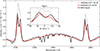 |
Fig. 1. Spatially averaged spectra of the Mg II h&k lines. Shown are the spectra from the MURaM-ChE simulation once computed in full 3D RT (red) and once using the plane-parallel 1.5D RT approximation (gray). For comparison, we show an observation from a qualitatively similar bipolar feature, which covers a similar area on the Sun (black). |
In the k2 peaks and k3 minimum, the 1.5D and 3D RT computations differ. The intensity of the k2v peak from the 3D average spectrum is 32% lower than the intensity of the k2v peak from the 1.5D average spectrum. Similarly, the k2r peak intensity in 3D RT is 41% lower than in the 1.5D RT computation. The central minimum in 3D RT is 42% lower than in the 1.5D RT computation. These values are almost a factor of four higher than the values we estimated in Pub I from the difference in the Bifrost public snapshot between 1.5D and 3D RT computations (see Sukhorukov & Leenaarts 2017, Fig. 10). This indicates that in the MURaM-ChE simulation, 3D RT effects are more important as they decrease the intensity contrast. In the k1 and h1 features, and in the pseudo-continuum between the Mg II h&k lines, the 3D RT and 1.5D RT computations agree with each other. While locally there can exist differences at these intensities, there seems to be no net effect when the spectrum is averaged over the whole cube. This is expected as these intensities form in the lower atmosphere, where 3D RT is less important. We further discuss the discrepancy between the 1.5D and 3D RT results in Sect. 3.1.2.
In comparison with the observed spectrum, the 3D RT computation results in a closer match of the line core; however, the k2 and h2 peak intensities are lower in the 3D RT computation. The k3 and h3 intensity approximately matches the observed value. The k3 minima of the synthetic spatially averaged spectra are shifted by −5.3 km s−1 (3D RT) and −5.6 km s−1 (1.5D RT) with respect to the rest wavelength of Mg II k, whereas in the observation the k3 feature is shifted by −2.3 km s−1. These values were determined through a parabolic fit around the k3 feature of the spatially averaged profile, that is they are not the average of k3 wavelength positions from single columns. We find that at the typical heights where the k3 features form in the atmosphere, the average velocity is a downflow, explaining the net red shift of the spatially averaged spectrum. We discuss these results in more detail in Sect. 3.2.2. The peak intensity ratios computed via
 (1)
(1)
(see, e.g., Leenaarts et al. 2013b, Eq. (2)) are 0.08 (1.5D RT), 0.16 (3D RT), and 0.09 (IRIS). This means for all three spectra the blue peak (Ik2v) is stronger than the red peak (Ik2r). The higher peak intensity ratio in the 3D RT computation than in the 1.5D RT computation is a result of the lower k2 intensities in 3D RT while the difference between two k2 peaks, that is Ik2v − Ik2r is similar for the two computations, that is 0.24 nJ m−2 s−1 Hz−1 sr−1 (3D RT) and 0.2 nJ m−2 s−1 Hz−1 sr−1 (1.5D RT). The peak intensity difference for the observations is 0.16 nJ m−2 s−1 Hz−1 sr−1.
The peak separations of the spatially averaged spectra are 32.18 km s−1 (IRIS), 22.41 km s−1 (3D RT), and 18.58 km s−1 (1.5D RT). The roughly 4 km s−1 higher value of the 3D RT vs. 1.5D RT computation demonstrates that horizontal velocities can have a visible effect on the peak separation (see also Sect. 3.1.2 and Appendix A). The remaining difference between the model and the observation might be explained by the known correlation between the peak separation and the maximum difference of the vertical velocity along the LOS, as for example shown in Fig. 8 in Leenaarts et al. (2013b), Fig. 5 in Pereira et al. (2013), or Fig. 6 in Pub I. This suggests that the vertical motions of the simulation presented here may be lower than in the real Sun. A more dynamic model atmosphere might be achieved by extending the simulation box in the horizontal directions to allow more interaction between the network elements and the quieter parts. In addition, a higher numerical resolution might lead to an increase in the chromospheric dynamics.
3.1.2. The role of horizontal velocities in the solution of the RT problem
In order to identify possible reasons for the discrepancy between the 1.5D and full 3D RT spectrum, we now discuss the Mg II k spectrum at a single location but with different settings used in the RT calculation. We randomly selected a location which showed a large difference in the k2 intensities between the full 3D and 1.5D RT calculation. First, we checked whether the different angular quadratures used by the 3D and 1.5D solvers have an effect on the spectrum. We therefore computed the spectrum at the selected location assuming a plane-parallel atmosphere but once using the Carlson (1963)-A4 angular quadrature (which is used by the 3D solver) and once with the Gauß-Legendre quadrature based on five angles (which is used by the 1.5D solver). As can be seen in Fig. 2a, there is no significant difference between the two computations, demonstrating that both specific quadratures are compatible in this example.
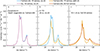 |
Fig. 2. Effect on the spectral line profile of varying the angular quadrature, and of including horizontal velocities (vh) in the RT computation. The figure shows profiles calculated from a single pixel of the simulation. In panel (a) we compare spectra computed assuming a plane-parallel atmosphere, neglecting horizontal velocities, with two different angular quadratures: the Gauß-Legendre (GL) quadrature and the Carlson (1963)-A4 quadrature. In panel (b) we compare the computations from the plane-parallel atmosphere without horizontal velocities with a computation that takes the horizontal velocities into account. In panel (c) we compare the computed spectrum from the 1D plane-parallel atmosphere with horizontal velocities with the spectrum computed in full 3D at the same location. |
Next, we tested whether the horizontal velocity field can have an impact on the resulting spectrum when the RTE is solved on the plane-parallel atmosphere. In the RH1.5D (Uitenbroek 2001; Pereira & Uitenbroek 2015) code, that we used in Pub I, and in the 1.5D solver of Multi3D the horizontal velocities are not taken into account. We therefore used the 3D solver of Multi3D but applied it to a plane-parallel atmosphere constructed from the selected location. By doing so, we can directly study the effect of the horizontal velocity field on the emergent spectrum in a de facto 1D RT computation. As shown in Fig. 2b the line profile is significantly affected by the horizontal velocities. The line is broadened and the k2 peak intensity is reduced. In panel (c) we compare the spectrum from the plane-parallel atmosphere (including horizontal velocities) with the full 3D RT solution that takes all inhomogenities of the 3D atmosphere into account. The line shape of the full 3D solution is even broader, and the peak intensities are slightly more reduced. Interestingly, the solution of the plane-parallel atmosphere with horizontal velocities is in this example closer to the full 3D solution than to the 1D RT computation without horizontal velocities (panel b). Especially the k2r peak results in nearly the same intensity. In Appendix A we present the net effect of the horizontal velocities on the spatially averaged spectrum and the statistical distributions of spectral line parameters by comparing the full 3D computation with a 3D computation where the horizontal velocities are set to zero. The results shown in Figs. A.1 and A.2 are similar: the horizontal velocities reduce the peak intensities and slightly increase the peak separation.
From this experiment, we conclude that the horizontal velocity field can have a significant impact on the resulting line shape, even when the spectra are computed in a plane-parallel atmosphere. This suggests the observed difference between the standard 1.5D RT calculation, that is without horizontal velocity field, and the full 3D RT solution as visible in Fig. 1 might therefore partly be a result of the dynamic horizontal velocity field in the MURaM-ChE EN model. This finding is similar to the result of Jaume Bestard et al. (2021) who studied the effect of the horizontal velocity field in the forward modeling of the Ca I 4227 Å line. We note that we calculated all presented spectra in Fig. 2 with full PRD. In the complete frequency redistribution (CRD) approximation, a similar effect is visible. However, the effect in CRD is reduced since CRD already broadens the line and lowers the k2 intensities (see, e.g., Sukhorukov & Leenaarts 2017, Fig. 10).
3.1.3. Intensity images of the observation and the synthesized snapshot
In this section, we compare the appearance of the intensity images at different spectral features such as the rest wavelength, k2 peaks, and k3 minimum. We aim to demonstrate how 3D RT affects the emergent intensity at different locations in the simulation snapshot and how this qualitatively compares with an observation of a bipolar magnetic structure. Figure 3 shows the intensity at the rest wavelength (first column, panels a, e, and i), at the k2v feature (second column, panels b, f, and j), the k3 feature (third column, panels c, g, and k), and the k2r feature (fourth column, panels d, h, and l). We compare the observations (top row) with results from our model combined with 3D RT (middle row), and computed spectra in the 1.5D RT approximation (bottom row).
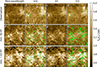 |
Fig. 3. Qualitative comparison with observations. We compare three different sets of intensity images. The first row shows the intensity map of the Mg II k line from the observation taken at the line-center rest wavelength (panel a), the k2v feature (panel b), the k3 feature (panel c), and the k2r feature (panel d). The second row (panels e, f, g, and h) shows the same quantities, but for the MURaM-ChE model using 3D RT calculations, and the bottom row (panels i,j,k, and l) when the RT problem is solved on a column-by-column approach. The selected region of interest (ROI) from the observation has the same FOV as the box size of the simulation. Green pixels indicate spatial locations where no feature could be detected by the peak-finding algorithm. The synthetic spectra were degraded and rebinned to the specifications of the observation dataset. |
The observed bipolar structure shows enhanced intensity above the network polarities in all spectral features. The intensity image at the rest wavelength (panel a) and k3 feature (panel b) shows fibril-like structures connecting the two polarities. The observed k2v image (panel b) shows shock-expansion patterns beneath the bipolar structure, that is, in the upper left and lower right corners of the image. The observed k2r image (panel d) shows less sharply defined shock-expansion patterns and is overall fainter. This suggests that the k2r peak forms at slightly different heights in the atmosphere than the k2v peak. The fact that the k2r image (panel d) is more “washed out” than k2v (panel b) might indicate that the red peak forms higher up in the atmosphere.
The intensity images computed with 3D RT (middle row, panels e–h) show similar features as the observation, such as connecting fibrilar structures between the polarities. However, they show a higher contrast at the rest wavelength and at the k3 feature than the observation. The 3D RT intensity images taken at the k2 peaks (panels f and h) show more structure and higher maximum intensities above the network magnetic fields than the observation (panels b and d). The contrast in the observed images might be lower due to the presence of stray light.
The intensity images from the 1.5D RT computations show two dominant differences compared with the 3D RT computation. First, the intensity above the network fields is much higher, and in the quiet region (upper left and lower right edges of the images), there exist much fainter regions. The second difference is that at the rest wavelength (panel i) and at the k3 feature (panel k), the fibrilar structures are hardly visible, whereas in the 3D RT computation (e.g., panel g), they are clearly visible.
3.1.4. Statistical comparison with the observation
Comparing an average spectrum can be overly influenced by the high-intensity pixels. We therefore study here the distribution of the spectral line features. In Fig. 4, we show distributions of peak brightness temperature (panel a), k2 peak separation (panel b), and k2 peak intensity ratio (panel c) of the computed spectra and the observations. The peak brightness temperature of the observation is on average 5.19 kK with minimum values of ≈4.75 kK and maximum values of ≈5.9 kK. The distribution has a Gaussian shape with an extended tail towards higher temperatures, similar to a log-normal distribution. Such log-normal distributions have also been found for the brightness at other wavelengths (Pauluhn et al. 2000). The distribution of the peak brightness temperatures from the 3D RT computations has a similar shape as the observation but slightly shifted towards lower temperatures. The mean is 5.12 kK, that is approximately 100 K lower than in the observed distribution. The minimum and maximum values are here ≈4.6 kK and 6.25 kK. The highest peak brightness temperature, however, has a very low occurrence. The results of the spectra computed with 1.5D RT are different in mainly two ways. First, the distribution is broader extending to lower (≈4.4 kK) and higher (≈6.5 kK) brightness temperatures. Second, the average brightness temperature of 5.34 kK from the 1.5D RT computation is higher than the 3D RT computation and the observation. This result demonstrates that in the MURaM-ChE simulation peak brightness temperatures higher than ≈5.25 kK are overestimated in the 1.5D RT approach.
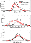 |
Fig. 4. Statistical comparison with observations. In panel (a) we show distributions of the k2 peak brightness temperature, in panel (b) the distribution of k2 peak separation, and in panel (c) the distribution of the k2 peak intensity ratio. We show data from the IRIS observation in black and data from the synthetic spectra computed by 3D RT in red, and 1.5D RT in gray after degradation to instrumental conditions. |
The observed peak separation distribution has an average value of 32.24 km s−1 and shows an approximately Gaussian shape; however, there are slightly more occurrences of higher values. The smallest observed values are ≈17 km s−1 and the largest are ≈45 km s−1. The peak separation distribution of the 3D RT spectra shows a slightly higher average of 26.62 km s−1 compared to the 1.5D RT spectra, which are on average 24.01 km s−1. The value of the 1.5D RT spectra is ≈0.6 km s−1 larger than what we found in Pub I, (Sect. 3.2.3.). This could be because of a difference in the codes, the smaller atom model, or the fact that we considered only every other column in the atmosphere for the RT computations here. The difference is small, however, compared for example to the wavelength resolution of IRIS, which is 2.4 km s−1. The peak-separation distribution of the 3D RT spectra seems to be shifted by 2 − 3 km s−1 toward higher values. This might be because the spectra computed in 3D RT have a smaller number of small peaks such that the peak separation is better defined. It may also be partly a result of horizontal velocities, which are taken into account in the full 3D RT synthesis, but not in the 1.5D RT synthesis (see Sect. 3.1.2).
We computed the peak intensity ratio (Eq. (1)) for the observation and the computed spectra. The corresponding distributions are shown in panel (c). The average values are 0.09 (IRIS), 0.09 (1.5D RT), and 0.12 (3D RT). These values compare to the ones estimated from the spatially averaged spectrum (Sect. 3.1.1). The peak intensity ratio is again largest for the 3D RT spectra. As described in Sect. 3.1.1, the difference between the 1.5D RT and 3D RT values might originate from the fact that in the peak intensity ratio, the differences are normalized by the sum of the intensities. Irrespective of whether the spectra are computed with 1.5D or 3D RT, the model produces broader distributions of the peak intensity ratio than in the observation.
3.2. Correlations between spectral line properties and the atmosphere
In this second part of our results, we study correlations between spectral line properties and atmospheric properties. The diagnostic potential of such correlations has been presented by Leenaarts et al. (2013b) and Pereira et al. (2013). Our aim is here to test whether similar correlations can be found in a different model of the solar chromosphere and how strongly they depend on the model. We begin with a discussion of intensity images at the k2v, k2r, and k3 features of the Mg II k line. We compare the intensity images to maps of the corresponding formation heights as well as vertical velocity, temperature, and density at the formation height. We then present correlations between the Doppler shifts of the k2 and k3 features and the vertical velocities at their formation heights. We further study the relationship between the peak intensity ratio and the average velocity between the formation height of the k2 peaks and the k3 feature. Finally, we test the potential of the k2 peak to infer chromospheric temperatures.
3.2.1. Images of synthetic intensity and atmospheric properties
The formation of spectral features of the Mg II h&k lines is known to depend on both the temperature and velocity field over a wide range of heights in the chromosphere. To demonstrate these relationships, we present in Fig. 5 intensity maps, formation heights, the vertical velocity, temperature, and density at the height of formation τν = 1 of the spectral feature in question (given at the top of the figure).
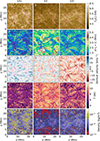 |
Fig. 5. Atmospheric properties at the formation height of the Mg II k spectral line features. Intensity maps (first row, panels a–c), formation heights (second row, panels d–f), vertical velocity maps (third row, panels g–i), temperature (fourth row, panels j–l), and density (fifth row, panels m–o). We show these quantities for the following spectral features: k2v (left column, panels a, d, g, j, and m); k3 (middle column, panels b, e, h, k, and n); and k2r (right column, panels c, f, i, l, and o). The synthetic spectra correspond to the snapshot muram_en_499000_379s. The pink pixels indicate where the respective spectral feature could not be detected by the peak-finding algorithm. |
We find the k2v peak shows different formation properties compared to the k2r peak. The intensity image of k2v (panel a) shows more shock expansion patterns throughout the whole simulation domain than in the k2r intensity image (panel c). Shock expansion patterns are web-like structures, similar to reversed granulation, of enhanced intensity of Tb > 6 kK. They are more clearly visible in the quiet regions of the simulation, that is at y ≤ 5 Mm and y ≥ 17 Mm. An example is visible at (x, y) = (5 Mm, 22 Mm) in panel (a). While similar structures exist in the k2r image (panel c), they are fainter and show different shapes. The k2r intensity image rather shows fibrillar structures of the upper chromosphere as traced by the k3 feature (panel b). This suggests k2v forms lower in the atmosphere than k2r. This is supported by the formation height maps shown in panel (d, k2v) and panel (f, k2r). There, it can be seen that at the same location, the k2r feature can form up to ≈1 Mm higher than k2v. In addition, the formation height image of k2r shows imprints of the loop-like structure of the upper chromosphere (see, e.g., panel e), whereas such structures are hardly visible in panel (d).
The comparison with the atmospheric properties shows additionally that the vertical velocity at the formation height of k2v (panel g) shows preferred upflows (i.e., 71% of the pixels) in relatively thin, spatially concentrated structures with an average velocity of ⟨vz(h(τk2v = 1))⟩ = 3.7 km s−1. In contrast, the vertical velocity at the formation height of k2r (panel i) traces downflows (in 86% of the pixels) in spatially more expanded structures with an average velocity of ⟨vz(h(τk2r = 1))⟩ = −7.3 km s−1. The vertical velocity map traced by the formation height of the k3 feature shows a rather balanced appearance of upflows (43%) and downflows (57%). The maps of temperature and density similarly highlight differences in the formation of k2v and k2r. The temperature map of k2v (panel j) shows lower atmospheric temperatures (on average 6.8 kK) but in regions of higher density, on average 3.58 × 10⁻⁸ kg m−3. Clearly visible in panel (m) is the web-like shock pattern in yellow color at densities of ≈10−7 kg m−3. In contrast, the temperature at the formation height of k2r is higher (on average 8 kK) and the density is lower (on average 6.7 × 10⁻⁹ kg m−3). The higher densities at the formation of k2v lead to a stronger coupling between the radiation field and the local gas temperature and thus result in higher peak intensities.
3.2.2. Correlation between Doppler shifts and vertical velocity at the formation height
We now study the diagnostic potential of the k2 and k3 Doppler shift in more detail. In Fig. 6 we show correlations between the Doppler shift and the vertical component of the atmospheric velocity for k2v (panel a), k3 (panel b), and k2r (panel c). The correlations based on the k2 features indicate a correlation such that the Doppler shift of k2v (k2r) correlates with upflows (downflows) at the corresponding height of formation in the atmosphere. The Pearson correlation coefficients are Rp = 0.66 (k2v) and Rp = 0.84 (k2r). The correlations of k2v and k2r are offset toward positive (k2v) and negative (k2r) Doppler velocities due to the location of the spectral features with respect to the line core. There are regions in panels (a) and (c) where the spectra show a large Doppler shift but the vertical velocity component in the atmosphere is small. These profiles are broad because of a peak in the temperature stratification in the lower atmosphere (see Pub I, Sect. 3.2.4.).
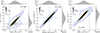 |
Fig. 6. Correlations between Doppler shift of spectral features of Mg II k and the vertical velocity in the atmosphere. Panel (a): Correlation between Doppler shift of k2v and the vertical component of the velocity at the formation height. Panel (b): Similar relation, but for k3. Panel (c): Same as panel (a), but for k2r. The Pearson correlation coefficient RP is given in each panel. The blue solid lines indicate x = 0 and y = 0. The black dashed line indicates x = y. The red, green, and blue contours enclose 25%,50%, and 90% of the data. |
The correlation between the Doppler shift of k3, and the atmospheric velocity at the formation height is tight with a Pearson correlation coefficient of RP = 0.94. This coefficient is slightly lower than the coefficient found by Leenaarts et al. (2013b), which was RP = 0.99. For their correlation, the authors computed the line core of Mg II h&k in 3D RT but under the CRD approximation. In Leenaarts et al. (2013b, Fig. 4) it can also be seen that ≈90% of the data points in the public Bifrost snapshot have vertical velocities within ±10 km s−1 at the formation height of k3. In the MURaM-ChE model, the distribution extends to ≈ ± 16 km s−1 (Fig. 6b, blue contour), and the scatter is larger. The average vertical velocity at the formation heights of the k3 feature is ⟨vz(h(τk3 = 1))⟩ = −1.25 km s−1 corresponding to an average Doppler shift of −1.23 km s−1, which is slightly different from the values obtained from the spatially averaged spectrum. This shows that the Doppler shift of the k3 feature inferred from the spatially averaged line profile does not necessarily reflect the average of the Doppler shifts of k3 features from single profiles (see also, Judge et al. 2020).
3.2.3. Correlation between peak intensity ratio and motions in the atmosphere
The peak intensity ratio (Eq. (1)) was shown by Leenaarts et al. (2013b) to be an indicator of the average vertical velocity in the atmosphere between the formation heights of the k2 peaks and k3. Due to the large difference between the formation heights of k2v and k2r we compute the average velocity not from the average k2 formation height but from the minimum of the two formation heights of k2v and k2r (see Pub I, Eqs. (2) and (3)). In addition, we exclude cells along the LOS with temperatures of Tgas > 12 kK as no significant contribution to the intensity is expected from there (see, e.g., Carlsson & Leenaarts 2012, Fig. 11). As shown in Fig. 7, we find a similar correlation to that found by Leenaarts et al. (2013b), that is, Ik2v > Ik2r is correlated with an average downflow in the atmosphere, and vice versa. Our distributions, however, show more scatter and a weaker Pearson correlation coefficient of RP = −0.33, compared to Leenaarts et al. (2013b) who found RP = −0.51. This results from a larger amount of complex spectral line profiles we find in the MURaM-ChE model than compared with the public Bifrost snapshot. Such spectral line profiles show more than two peaks and thus introduce a certain degree of ambiguity for the peak-finding algorithm. The more complex spectral line profiles are a result of the more dynamic atmosphere in the MURaM-ChE model than in the public Bifrost snapshot (see, e.g., Pub I, Fig. 11b). Another contribution to the scatter could come from the fact that the topology of the chromosphere in the MURaM-ChE simulation is rather complex, sometimes with hot (T > 12 kK) gas lying between the formation heights of the k2 and k3 features (see also Pub I, Fig. 7c), making a definition of an “average velocity” in the considered height range difficult.
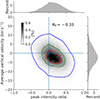 |
Fig. 7. Correlation between peak intensity ratio and average vertical velocity. The average vertical velocity is measured from the minimum formation height of the two k2 features and the formation height of the k3 feature. The red, green, and blue contours enclose 25%,50%, and 90% of the data. The blue solid lines indicate x = 0 and y = 0. |
3.2.4. Temperature diagnostics
Another diagnostic property of the Mg II h&k lines is the correlation between the peak brightness temperature and the atmospheric temperature at the formation heights (see Leenaarts et al. 2013b, Figs. 6e and f). This correlation, however, tends to be only valid for intensities above a certain minimum brightness temperature of ≈5 kK. These intensities are formed at heights in the chromosphere where the source function is still sufficiently coupled to the local gas temperature.
We studied the same correlations and present them in Fig. 8. In panel (a) we show the results for the k2v feature. It can be seen that there is a correlation between brightness temperatures of Tb > 5.25 kK with the plasma temperature. However, the Pearson correlation coefficient is only RP = 0.12. The reason is that already at the formation height of the k2v peak, the line source function can be decoupled from the local gas temperature. The Pearson correlation coefficient for all datapoints in Fig. 8a is negative (RP = −0.15). For Tb < 5.25 kK, there is a large variety of atmospheric temperatures, which result in a rather narrow range of brightness temperatures of Tb ≈ 4.75 kK to Tb ≈ 5 kK. These intensities form between the shock-like patterns at a slightly higher formation height. Such scenarios can, for example, be seen in Fig. 5 (a, brightness temperature) and (d, formation height). There is a cluster of datapoints at Tgas ≈ 10 kK where the intensity is decoupled from the local temperature. The maximum atmospheric temperatures of roughly 12 kK indicate the maximum temperatures where Mg II exists dominantly (Carlsson & Leenaarts 2012, Fig. 11).
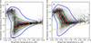 |
Fig. 8. Correlation between peak brightness temperatures and temperature at the formation height in the atmosphere. Panel (a) shows the correlation for the blue peak (k2v) and panel (b) shows the correlation for the red peak (k2r). The red, green, and blue contours enclose regions of 25%,50%, and 90% of the data. The orange lines indicate x = y. We normalized each column of brightness temperature to the maximum value of atmospheric temperature in that column. |
In panel (b), we show the correlation for the k2r peak. There is a similar but less tight correlation for Tb > 5.25 kK with a Pearson correlation coefficient of Rp = 0.06. The maximum brightness temperatures of k2r are lower than those of k2v, which was already indicated in the average spectrum (see Fig. 1). For brightness temperatures of Tb < 5.25 kK the correlation is even lower. The overall correlation coefficient is RP = −0.21, which is more negative than for k2v. This can be understood from the fact that in our model k2r forms higher in the atmosphere than k2v, at lower densities and therefore is less suitable to estimate the atmospheric temperature.
Our results compare with the findings of Leenaarts et al. (2013b, Figs. 6e and f). These authors found a stronger intensity-temperature correlation for the k2v peak than for the k2r peak. The actual Pearson correlation coefficients are similarly low. In the public Bifrost snapshot, there is a larger fraction of brightness temperatures below 4.7 kK. The differences of the temperature stratification between the Bifrost public snapshot and the MURaM-ChE model were discussed in Pub I, Fig. 11a and Sect. 3.3 where the authors found higher temperature in the MURaM-ChE model at the formation heights of Mg II k in the chromosphere.
4. Summary and discussion
In this work, we analyzed the spectral line properties of the Mg II h&k lines using 3D RT computations in a simulation of a bipolar magnetic feature in the solar atmosphere computed with the MURaM-ChE code. In previous work (Pub I), we analyzed the Mg II h&k lines of the same simulation snapshot in 1.5D RT. Here we discuss the combined results and compare them with previous work.
We determined the spatially averaged spectra, intensity images of the spectral line features, and statistical distributions of line parameters from 1.5D RT and 3D RT computations and from a dataset recorded by the IRIS spacecraft and compared the results from these three sources. We also compared with previous results for the same spectral lines obtained from Bifrost simulations. The FOV of the observation was chosen to include a similar bipolar magnetic feature as in the simulation.
We found that the distribution of the k2 and k3 intensities cover a much wider range and in general display larger values for the 1.5D RT computation than for the 3D RT computation. Therefore, for the spatially averaged spectrum these intensities are up to 72% higher in the profile obtained via 1.5D RT than in the profile from 3D RT computations. Thus, in the MURaM-ChE model, the effects of 3D RT are important not only in the k3 minimum but in the whole line inside the k1 minima. While Sukhorukov & Leenaarts (2017, Fig. 10) found similar results for computations with the public Bifrost snapshot, the difference between the 1.5D RT and 3D RT spatially averaged spectra was much smaller (approximately 12% for k2r). In the 1.5D RT MURaM-ChE computation, the k2 intensities are most strongly overestimated above the network fields. There, the formation heights of k2 are relatively low (< 1.5 Mm, see for example Figs. 5d and f), such that higher densities lead to a stronger coupling between the radiation field to the local temperature and, thus higher emergent intensities. In the plane-parallel RT approximation, the horizontal gradients in density and temperature that connect the network-dominated region with the quieter part of the simulation are neglected, which may partly lead to the overestimation.
In addition, in Fig. 2 and Appendix A, we demonstrate that the horizontal velocities can have a significant effect on the line shape and especially the k2 intensities. This is in agreement with Jaume Bestard et al. (2021) who found that horizontal velocities in 1.5D improve the RT calculation towards the full 3D solution. While these authors studied the Ca I 4227 Å in the CRD approximation, we found that for the Mg II h&k lines the effect is even more strongly visible in the PRD computation. The relative difference between the 3D vs. 1.5D spatially averaged spectra, which is larger in the MURaM-ChE EN than for the public Bifrost snapshot (see Sukhorukov & Leenaarts 2017, Fig. 10), might therefore also be a result of the different horizontal velocity fields in the two atmosphere models.
The distribution of brightness temperature of the k2 peaks in the 3D RT computation compares much better to the observed distribution than the 1.5D RT case (see Fig. 4a). The strength of the averaged profile is also closer to the observations, although it is now (3D RT) slightly underestimated; however, the absolute strength of the profile depends on the exact amount of magnetic flux in the simulation and the observation (see Pub I).
We found that 3D RT produces a slightly higher peak separation of the spatially averaged spectrum than the 1.5D RT computation. This can also be seen in the distributions of the peak separation from single spectra (see Fig. 4b). In Appendix A we show that this is also an effect of the horizontal velocities that are taken into account in the full 3D computation. Typical 1.5D RT computations instead take only the vertical velocity component into account. A better match between the model and the observation might be achieved by a simulation that includes a similar magnetic bipole, but has a larger horizontal extent to allow more interaction with the quiet part in the simulation. This might lead to a more dynamic atmosphere and possibly higher mass loading, which can have an effect on the line width (see, e.g., Hansteen et al. 2023). In addition, a higher numerical resolution might lead to a more dynamic atmosphere (see, e.g., Carlsson et al. 2016; Hansteen et al. 2023).
The peak intensity ratio is even higher in 3D RT, making it a worse match to the observations. The too high peak intensity ratio in the 3D RT computations could be due to either a too high k2v or a too low k2r intensity. As we found in Sect. 3.2.1, the k2r peak forms higher in the atmosphere than k2v. A too low k2r intensity could be due to multiple reasons. For example, a higher gas density at the k2r formation height might increase the intensity through a stronger coupling to the local temperature. As we found in Sect. 3.2.1 and Figs. 5m and o, the density at the formation height of k2v can be up to two orders of magnitude higher than at the formation height of k2r. Another contribution to the peak intensity ratio occurs due to the velocity structure in the atmosphere. Similar to the findings of Carlsson & Stein (1997), the k2v peak is stronger than k2r if the local atmosphere above the formation heights of the peaks is moving on average downwards, leading to a positive peak intensity ratio (and vice versa). Such a correlation was found by Leenaarts et al. (2013b) for the Mg II h&k lines in the public Bifrost snapshot. The correlation in the MURaM-ChE simulation shows more scatter, however. This might be a result of the more dynamic atmosphere, that is, there exists much more variation in vertical velocity along the line of sight. While we showed here only the results of one synthesized snapshot, it is not immediately clear whether the spectral line properties, such as peak asymmetry, are time-dependent in the simulation. In Pub I, we estimated the spatially averaged spectrum from a lower spatial but higher time resolution computation by synthesizing eight slits in the simulation. There, we found not much variation in the spatially averaged line width, peak intensity, and peak intensity ratio over time.
In addition to this, we checked here whether oscillations in the simulation box affect the flow structure in the chromosphere. In Fig. 9, we show the average vertical velocity as a function of height and time (panel a), the average height of the τ500 = 1 surface as a function of time (panel b), and the average vertical velocity at the approximate formation heights of the k2 features (panel c). We find the average τ500 = 1 height changes periodically within ≈6 min with an amplitude of ≈3–4 km. The oscillation seems to correlate with the average vertical velocity in the lower chromosphere (z < 1 Mm). Higher up in the chromosphere at 1.7 Mm ≤ z ≤ 2.7 Mm, approximately the heights between where the k2v and k3 features form, the atmosphere shows on average downflows independent of time. In panel (c) we show the average vertical velocity in the atmosphere averaged over the whole xy-plane between heights of z = 1.7 Mm and z = 2.7 Mm. It can be seen that these velocities are always negative between ≈ − 2.6 km s−1 and ≈ − 4.3 km s−1. Therefore, in accordance with Fig. 7 and the results from Leenaarts et al. (2013b, Fig. 8g), it might be that there is a positive peak asymmetry ratio in the spatially averaged spectrum at almost any snapshot in the simulation. We note, however, as discussed above, that other atmospheric parameters play an important role in line formation, in addition to the velocity field.
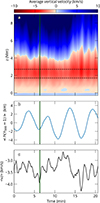 |
Fig. 9. Time-dependent velocity structure in the atmosphere. Panel (a) shows the average velocity as a function of height. Panel (b) shows the time-dependent average height of the τ500 = 1 surface. Panel (c) shows the average vertical velocity between z = 1.7 Mm and z = 2.7 Mm, which are the average formation heights of the k2v feature and k3 feature in the snapshot presented here. |
We found that correlations between spectral line properties and the atmosphere exist similarly to the findings of Leenaarts et al. (2013b) and Pereira et al. (2013). We could confirm that a tight correlation between the vertical velocity at the formation height of k3 and the Doppler shift of this spectral feature exists. In addition, we found that the Doppler shifts k2v (k2r) correlate preferentially with upflows (downflows). This means the k2v and k2r peaks of the same ray may probe significantly different layers of the atmosphere. In particular, we found k2v traces lower-lying regions of higher density, probably due to shock compression. Whereas k2r forms higher up at lower densities and on average at larger velocities.
The k2 peak intensity as a temperature diagnostic is only partly valid in the MURaM-ChE simulation. We found, in general agreement with Leenaarts et al. (2013b), that for k2v peak brightness temperatures > 5.25 kK, there seems to be a good correlation. However, the Pearson coefficient is relatively low (0.12). In the case of k2r, this correlation is weaker with a Pearson correlation coefficient of 0.06, which can be understood by our findings that k2r forms higher up in the chromosphere, where NLTE effects become more important.
As a general result, we find the MURaM-ChE model is able to produce a close match to the observed line width in 1.5D RT and 3D RT at a relatively moderate resolution of 23.4 km (horizontal) and 20 km (vertical). Whether a higher resolution will improve the match with the observation needs to be shown in the future.
5. Conclusion
We performed 3D RT computations with the Multi3D code in an EN simulation that was computed with the MURaM-ChE code. We confirmed that the effects of horizontal RT must be taken into account to accurately model the Mg II h&k lines. The difference between 1.5D RT and 3D RT was even more pronounced than in previous studies with the public Bifrost snapshot. In addition, we confirmed the diagnostic potential of the Mg II k line to constrain the velocity structure of observations. We found that k2v and k2r trace different features in the chromosphere, which might help to better interpret observed spectra. While differences still exist between the 3D RT computations of the Mg II h&k lines and the observation, our results demonstrate progress in the numerical modeling of the chromosphere.
Acknowledgments
We thank the anonymous referee for comments and suggestions that improved the quality of this paper. This work was supported by the International Max-Planck Research School (IMPRS) for Solar System Science at the University of Göttingen. This work received funding from the European Research Council (ERC) under the European Union’s Horizon 2020 research and innovation programme (grant agreement No. 101097844-project WINSUN). This research has received financial support from the European Union’s Horizon 2020 research and innovation program under grant agreement No. 824135 (SOLARNET). This work was supported by the Deutsches Zentrum für Luft und Raumfahrt (DLR; German Aerospace Center) by grant DLR-FKZ 50OU2201. We highly appreciate the computing resources provided by the HPC systems Raven, Cobra, and Viper at the Max Planck Computing and Data Facility.
References
- Avrett, E., Landi, E., & McKillop, S. 2013, ApJ, 779, 155 [NASA ADS] [CrossRef] [Google Scholar]
- Bjørgen, J. P., Sukhorukov, A. V., Leenaarts, J., et al. 2018, A&A, 611, A62 [Google Scholar]
- Bjørgen, J. P., Leenaarts, J., Rempel, M., et al. 2019, A&A, 631, A33 [Google Scholar]
- Bonnet, R. M., Decaudin, M., Bruner, E. C., Jr., Acton, L. W., & Brown, W. A. 1980, ApJ, 237, L47 [NASA ADS] [CrossRef] [Google Scholar]
- Carlson, B. 1963, Methods Comput. Phys. [Google Scholar]
- Carlsson, M., & Leenaarts, J. 2012, A&A, 539, A39 [NASA ADS] [CrossRef] [EDP Sciences] [Google Scholar]
- Carlsson, M., & Stein, R. F. 1997, ApJ, 481, 500 [Google Scholar]
- Carlsson, M., Hansteen, V. H., Gudiksen, B. V., Leenaarts, J., & De Pontieu, B. 2016, A&A, 585, A4 [NASA ADS] [CrossRef] [EDP Sciences] [Google Scholar]
- Carlsson, M., De Pontieu, B., & Hansteen, V. H. 2019, ARA&A, 57, 189 [Google Scholar]
- de la Cruz Rodríguez, J., & van Noort, M. 2017, Space Sci. Rev., 210, 109 [Google Scholar]
- De Pontieu, B., Title, A. M., Lemen, J. R., et al. 2014, Sol. Phys., 289, 2733 [Google Scholar]
- del Toro Iniesta, J. C., & Ruiz Cobo, B. 2016, Liv. Rev. Sol. Phys., 13, 4 [Google Scholar]
- Gošić, M., de la Cruz Rodríguez, J., De Pontieu, B., et al. 2018, ApJ, 857, 48 [CrossRef] [Google Scholar]
- Gudiksen, B. V., Carlsson, M., Hansteen, V. H., et al. 2011, A&A, 531, A154 [NASA ADS] [CrossRef] [EDP Sciences] [Google Scholar]
- Hannah, I. G., Kleint, L., Krucker, S., et al. 2019, ApJ, 881, 109 [NASA ADS] [CrossRef] [Google Scholar]
- Hansteen, V. H., Martinez-Sykora, J., Carlsson, M., et al. 2023, ApJ, 944, 131 [NASA ADS] [CrossRef] [Google Scholar]
- Jaume Bestard, J., Trujillo Bueno, J., Štěpán, J., & del Pino Alemán, T. 2021, ApJ, 909, 183 [NASA ADS] [CrossRef] [Google Scholar]
- Judge, P. G., Kleint, L., Leenaarts, J., Sukhorukov, A. V., & Vial, J.-C. 2020, ApJ, 901, 32 [Google Scholar]
- Kayshap, P., Tripathi, D., Solanki, S. K., & Peter, H. 2018, ApJ, 864, 21 [NASA ADS] [CrossRef] [Google Scholar]
- Leenaarts, J., & Carlsson, M. 2009, ASPC, 415, 87 [Google Scholar]
- Leenaarts, J., Carlsson, M., Hansteen, V., & Rouppe van der Voort, L. 2009, ApJ, 694, L128 [NASA ADS] [CrossRef] [Google Scholar]
- Leenaarts, J., Carlsson, M., & Rouppe van der Voort, L. 2012, ApJ, 749, 136 [NASA ADS] [CrossRef] [Google Scholar]
- Leenaarts, J., Pereira, T. M. D., Carlsson, M., Uitenbroek, H., & De Pontieu, B. 2013a, ApJ, 772, 89 [NASA ADS] [CrossRef] [Google Scholar]
- Leenaarts, J., Pereira, T. M. D., Carlsson, M., Uitenbroek, H., & De Pontieu, B. 2013b, ApJ, 772, 90 [NASA ADS] [CrossRef] [Google Scholar]
- Martínez-Sykora, J., de la Cruz Rodríguez, J., Gošić, M., et al. 2023, ApJ, 943, L14 [CrossRef] [Google Scholar]
- Milkey, R. W., & Mihalas, D. 1974, ApJ, 192, 769 [NASA ADS] [CrossRef] [Google Scholar]
- Ondratschek, P., Przybylski, D., Smitha, H. N., et al. 2024, A&A, 692, A6 [NASA ADS] [CrossRef] [EDP Sciences] [Google Scholar]
- Pauluhn, A., Solanki, S. K., Rüedi, I., Landi, E., & Schühle, U. 2000, A&A, 362, 737 [NASA ADS] [Google Scholar]
- Peat, A. W., Labrosse, N., Schmieder, B., & Barczynski, K. 2021, A&A, 653, A5 [NASA ADS] [CrossRef] [EDP Sciences] [Google Scholar]
- Pereira, T. M. D., & Uitenbroek, H. 2015, A&A, 574, A3 [NASA ADS] [CrossRef] [EDP Sciences] [Google Scholar]
- Pereira, T. M. D., Leenaarts, J., De Pontieu, B., Carlsson, M., & Uitenbroek, H. 2013, ApJ, 778, 143 [NASA ADS] [CrossRef] [Google Scholar]
- Przybylski, D., Cameron, R., Solanki, S. K., et al. 2022, A&A, 664, A91 [NASA ADS] [CrossRef] [EDP Sciences] [Google Scholar]
- Przybylski, D., Cameron, R., Solanki, S. K., et al. 2025, A&A, 703, A148 [NASA ADS] [CrossRef] [EDP Sciences] [Google Scholar]
- Rybicki, G. B., & Hummer, D. G. 1991, A&A, 245, 171 [NASA ADS] [Google Scholar]
- Rybicki, G. B., & Hummer, D. G. 1992, A&A, 262, 209 [NASA ADS] [Google Scholar]
- Scherrer, P. H., Schou, J., Bush, R. I., et al. 2012, Sol. Phys., 275, 207 [Google Scholar]
- Schmit, D., Bryans, P., De Pontieu, B., et al. 2015, ApJ, 811, 127 [NASA ADS] [CrossRef] [Google Scholar]
- Schou, J., Scherrer, P. H., Bush, R. I., et al. 2012, Sol. Phys., 275, 229 [Google Scholar]
- Štěpán, J., del Pino Alemán, T., & Trujillo Bueno, J. 2022, A&A, 659, A137 [NASA ADS] [CrossRef] [EDP Sciences] [Google Scholar]
- Sukhorukov, A. V., & Leenaarts, J. 2017, A&A, 597, A46 [NASA ADS] [CrossRef] [EDP Sciences] [Google Scholar]
- Uitenbroek, H. 2001, ApJ, 557, 389 [Google Scholar]
- Vernazza, J. E., Avrett, E. H., & Loeser, R. 1981, ApJS, 45, 635 [Google Scholar]
- Withbroe, G. L., & Noyes, R. W. 1977, ARA&A, 15, 363 [Google Scholar]
Max Planck Institute for Solar System Research/University of Chicago Radiation Magneto-hydrodynamics with the chromospheric extension.
Appendix A: The effect of horizontal velocities on the Mg II h&k lines
In this appendix, we demonstrate the effect of the horizontal velocities on the spatially averaged line profile and on single profiles computed at the disk center. In Fig. A.1, we show spatially averaged profiles resulting from the 1.5D RT, 3D RT without horizontal velocities, and the full 3D RT computation. It can be seen that the difference between the 1.5D RT and the full 3D RT computation is partly due to inhomogeneities in atmospheric quantities such as temperature or density, but also that the horizontal velocity field plays an important role. The 3D RT computation without horizontal velocities results in a slightly smaller peak separation and higher peak intensities than the full 3D computation. The same results can be seen by looking at the statistical distributions of the spectral line parameters as presented in Fig. A.2, which is similar to Fig. 4 in the main text, but additionally contains the results of the 3D RT computation with horizontal velocities set to zero. The distribution of the peak brightness temperature is shifted towards higher values in the 3D RT computation without horizontal velocities compared to the 3D RT computation taking the full atmosphere into account. The distribution of the peak separation computed without horizontal velocities is similar to the 1.5D RT computation, that does by default not take horizontal velocities into account. Finally, the distribution of the peak intensity ratio is only slightly affected by the horizontal velocities.
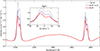 |
Fig. A.1. Effect of horizontal velocities on the spatially averaged line profile. We show the results of three different computations. In gray: 1.5D RT, computed without horizontal velocities. In purple: 3D RT, but computed without horizontal velocities. In red: 3D RT computation that takes the full atmosphere into account. |
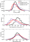 |
Fig. A.2. Effect of horizontal velocities on the distributions of spectral line parameters. The layout is identical to Fig. 4. Panel (a) shows the distributions of peak brightness temperature, panel (b) the distributions of peak separation, and panel (c) the distribution of the peak intensity ratio. In addition, we show in purple the results from the 3D RT computation where the horizontal velocities are set to zero. |
All Figures
|
Fig. 1. Spatially averaged spectra of the Mg II h&k lines. Shown are the spectra from the MURaM-ChE simulation once computed in full 3D RT (red) and once using the plane-parallel 1.5D RT approximation (gray). For comparison, we show an observation from a qualitatively similar bipolar feature, which covers a similar area on the Sun (black). |
| In the text | |
|
Fig. 2. Effect on the spectral line profile of varying the angular quadrature, and of including horizontal velocities (vh) in the RT computation. The figure shows profiles calculated from a single pixel of the simulation. In panel (a) we compare spectra computed assuming a plane-parallel atmosphere, neglecting horizontal velocities, with two different angular quadratures: the Gauß-Legendre (GL) quadrature and the Carlson (1963)-A4 quadrature. In panel (b) we compare the computations from the plane-parallel atmosphere without horizontal velocities with a computation that takes the horizontal velocities into account. In panel (c) we compare the computed spectrum from the 1D plane-parallel atmosphere with horizontal velocities with the spectrum computed in full 3D at the same location. |
| In the text | |
|
Fig. 3. Qualitative comparison with observations. We compare three different sets of intensity images. The first row shows the intensity map of the Mg II k line from the observation taken at the line-center rest wavelength (panel a), the k2v feature (panel b), the k3 feature (panel c), and the k2r feature (panel d). The second row (panels e, f, g, and h) shows the same quantities, but for the MURaM-ChE model using 3D RT calculations, and the bottom row (panels i,j,k, and l) when the RT problem is solved on a column-by-column approach. The selected region of interest (ROI) from the observation has the same FOV as the box size of the simulation. Green pixels indicate spatial locations where no feature could be detected by the peak-finding algorithm. The synthetic spectra were degraded and rebinned to the specifications of the observation dataset. |
| In the text | |
|
Fig. 4. Statistical comparison with observations. In panel (a) we show distributions of the k2 peak brightness temperature, in panel (b) the distribution of k2 peak separation, and in panel (c) the distribution of the k2 peak intensity ratio. We show data from the IRIS observation in black and data from the synthetic spectra computed by 3D RT in red, and 1.5D RT in gray after degradation to instrumental conditions. |
| In the text | |
|
Fig. 5. Atmospheric properties at the formation height of the Mg II k spectral line features. Intensity maps (first row, panels a–c), formation heights (second row, panels d–f), vertical velocity maps (third row, panels g–i), temperature (fourth row, panels j–l), and density (fifth row, panels m–o). We show these quantities for the following spectral features: k2v (left column, panels a, d, g, j, and m); k3 (middle column, panels b, e, h, k, and n); and k2r (right column, panels c, f, i, l, and o). The synthetic spectra correspond to the snapshot muram_en_499000_379s. The pink pixels indicate where the respective spectral feature could not be detected by the peak-finding algorithm. |
| In the text | |
|
Fig. 6. Correlations between Doppler shift of spectral features of Mg II k and the vertical velocity in the atmosphere. Panel (a): Correlation between Doppler shift of k2v and the vertical component of the velocity at the formation height. Panel (b): Similar relation, but for k3. Panel (c): Same as panel (a), but for k2r. The Pearson correlation coefficient RP is given in each panel. The blue solid lines indicate x = 0 and y = 0. The black dashed line indicates x = y. The red, green, and blue contours enclose 25%,50%, and 90% of the data. |
| In the text | |
|
Fig. 7. Correlation between peak intensity ratio and average vertical velocity. The average vertical velocity is measured from the minimum formation height of the two k2 features and the formation height of the k3 feature. The red, green, and blue contours enclose 25%,50%, and 90% of the data. The blue solid lines indicate x = 0 and y = 0. |
| In the text | |
|
Fig. 8. Correlation between peak brightness temperatures and temperature at the formation height in the atmosphere. Panel (a) shows the correlation for the blue peak (k2v) and panel (b) shows the correlation for the red peak (k2r). The red, green, and blue contours enclose regions of 25%,50%, and 90% of the data. The orange lines indicate x = y. We normalized each column of brightness temperature to the maximum value of atmospheric temperature in that column. |
| In the text | |
|
Fig. 9. Time-dependent velocity structure in the atmosphere. Panel (a) shows the average velocity as a function of height. Panel (b) shows the time-dependent average height of the τ500 = 1 surface. Panel (c) shows the average vertical velocity between z = 1.7 Mm and z = 2.7 Mm, which are the average formation heights of the k2v feature and k3 feature in the snapshot presented here. |
| In the text | |
|
Fig. A.1. Effect of horizontal velocities on the spatially averaged line profile. We show the results of three different computations. In gray: 1.5D RT, computed without horizontal velocities. In purple: 3D RT, but computed without horizontal velocities. In red: 3D RT computation that takes the full atmosphere into account. |
| In the text | |
|
Fig. A.2. Effect of horizontal velocities on the distributions of spectral line parameters. The layout is identical to Fig. 4. Panel (a) shows the distributions of peak brightness temperature, panel (b) the distributions of peak separation, and panel (c) the distribution of the peak intensity ratio. In addition, we show in purple the results from the 3D RT computation where the horizontal velocities are set to zero. |
| In the text | |
Current usage metrics show cumulative count of Article Views (full-text article views including HTML views, PDF and ePub downloads, according to the available data) and Abstracts Views on Vision4Press platform.
Data correspond to usage on the plateform after 2015. The current usage metrics is available 48-96 hours after online publication and is updated daily on week days.
Initial download of the metrics may take a while.