


| Issue |
A&A
Volume 709, May 2026
|
|
|---|---|---|
| Article Number | A251 | |
| Number of page(s) | 9 | |
| Section | Stellar structure and evolution | |
| DOI | https://doi.org/10.1051/0004-6361/202659029 | |
| Published online | 25 May 2026 | |
Fundamental properties of two rapidly rotating stars: Rasalhague and Alkaid
IRAP, Université de Toulouse, CNRS, CNES, 14, avenue Édouard Belin, F-31400 Toulouse, France
★ Corresponding author: This email address is being protected from spambots. You need JavaScript enabled to view it.
Received:
19
January
2026
Accepted:
6
April
2026
Abstract
Context. The fundamental parameters of rapidly rotating stars are key quantities required to understand the impact of rotation on stellar evolution. A few nearby early-type stars offer the possibility to take precise measurements of these parameters, which helped us to constrain newly available two-dimensional models.
Aims. We propose a method to retrieve the fundamental parameters of a fast-rotating star (mass, rotation rate, and age) and the inclination of its rotation axis on the line of sight using five spectrophotometric observables along with a set of steady 2D models.
Methods. From two photometric indices, the temperature TIRFM derived by the infrared flux method, the projected equatorial velocity (V sin i), and the apparent luminosity, along with a grid of 2D steady-state models, we selected models that are compatible with all observational constraints and derived the most probable mass, rotation rate, core hydrogen mass fraction relative to that of the envelope, and inclination of the rotation axis on the line of sight of the targeted star.
Results. We applied this method to two stars: Rasalhague (α Oph, A5IV) and Alkaid (η UMa, B3V). We confirm and improve on the fundamental parameters of Rasalhague previously determined by infrared interferometry and provide a new determination of its rotation axis inclination on the line of sight, which we find to be 68.9 ± 5.6°. Concerning Alkaid, about which little is known, we infer a mass of 5.071 ± 0.023 M⊙ and a rotation rate of 0.413 ± 0.057 times the critical angular velocity, corresponding to an equatorial rotation period of 14.6 hours. We also find an inclination of the rotation axis of 41.9 ± 8.2° on the line of sight. We show that Alkaid is a very young star, presumably between 2 and 8 Myr off the zero-age main sequence. As a side result, using high resolution spectra and the Least Square Deconvolution method, we determined a precise value of the V sin i of Rasalhague, namely 224.3 ± 2.6 km/s. Similarly, we find V sin i = 154.3 ± 9.1 km/s for Alkaid.
Conclusions. Our results show that fundamental parameters of rapidly rotating stars can be determined (or at least bracketed) using five observable quantities that can be measured from the spectrum of the star. This is of great interest for stars that are beyond reach of interferometric observations.
Key words: stars: fundamental parameters / stars: rotation
© The Authors 2026
 Open Access article, published by EDP Sciences, under the terms of the Creative Commons Attribution License (https://creativecommons.org/licenses/by/4.0), which permits unrestricted use, distribution, and reproduction in any medium, provided the original work is properly cited.
This article is published in open access under the Subscribe to Open model. This email address is being protected from spambots. You need JavaScript enabled to view it. to support open access publication.
1. Introduction
About 50% of early-type stars exhibit fast rotation (i.e. equatorial velocity higher than 100 km/s) according to Zorec & Royer (2012). For such stars, rotational evolution is a key aspect of their global evolution, which is driven by nuclear reactions. It is indeed associated with rotational mixing, which impacts both the surface abundances and the lifetime of the star by fuelling the convective core with hydrogen. In fact, the interface region between the core and the radiative envelope is also the place probed by gravity modes, for instance in γ Doradus or slowly pulsating B stars (e.g. Mombarg et al. 2022). Their oscillation spectrum is therefore much affected by the mixing around it (e.g. Burssens et al. 2023). However, the impacts of processes associated with rotation are still not well understood. Fast rotation makes them important and implies the use of two-dimensional models, which can deal with the oblate shape of the star, the large-scale baroclinic flows, and anisotropic transport. A step forward was accomplished with the release of the ESTER1 code that can compute two-dimensional models including all these effects (Espinosa Lara & Rieutord 2013; Rieutord et al. 2016; Mombarg et al. 2023). However, as for any model, we now need precise observational constraints to keep the models on the right track and ensure that predictions are correct.
Observables derived from stellar spectra have long been key quantities used to infer the fundamental parameters of stars. When rotation is fast, the spectral energy distribution (SED) is more complex to interpret, but it also contains more information since it is influenced by the so-called gravity darkening, which makes the polar regions brighter than the equatorial ones (Espinosa Lara & Rieutord 2011). Provided the use of realistic enough models, it is possible to tightly constrain the fundamental parameters of a fast-rotating star. This was the challenge taken up by Lazzarotto et al. (2023). Indeed, taking advantage of gravity darkening, these authors developed a method that uses photometric quantities to retrieve some fundamental parameters of a rotating star such as mass and rotation rate together with the inclination of the rotation axis. They combined ESTER models, PHOENIX atmospheric structures, and synthetic spectra (Hauschildt et al. 1999) to produce SEDs. As a validation test, they determined the fundamental parameters and inclination of Vega, with a very good agreement with previous determinations. However, they assumed an evolutionary status of the star as given by Vega’s concordance model of Monnier et al. (2012).
In the present work, we wished to go further and determine the age of the star. However, we restricted our study to early-type stars because they have convective cores, the hydrogen mass fraction of which can be used as a proxy of the evolutionary status. In addition, we also wished to compare our determination of the equatorial radius to that obtained by interferometric observations, if available. To this end, we considered two stars: Rasalhague (α Oph) and Alkaid (η UMa). Rasalhague2 is a nearby star located 14.8 pc from the Sun (Gardner et al. 2021) that has been observed with interferometers (Zhao et al. 2009; Baines et al. 2018, 2025) and with polarimetry (Bailey et al. 2020). Its mass and rotation rate make it a priori similar to Vega, but seen almost equator on, according to Zhao et al. (2009). Hence, expectedly, gravity darkening makes it of a later type than Vega along with a higher luminosity class, namely A5IVnn (Gray et al. 2001) versus A0V for Vega (Negueruela et al. 2024). The suffix ‘nn’ following the luminosity class means ‘very broad lines’ (e.g. Abt & Morrell 1995), which is consistent with a rapidly rotating star seen equator-on. It is therefore an interesting case to test a method based on gravity-darkening effects. The second star, Alkaid, was chosen essentially because its SED is accurately known from space data and available through the CALSPEC database (Bohlin & Lockwood 2022). As a hot star (spectral type B3V; Negueruela et al. 2024), it also allowed us to test our method in this range of effective temperatures, and we hope to give new reliable values of its fundamental parameters. We note that its angular diameter has also been estimated via interferometry (Baines et al. 2018; Gordon et al. 2019; Abe et al. 2024; Baines et al. 2025).
The paper is organised as follows: we first give an overview of our method in Sect. 2 and then discuss the cases of Rasalhague and Alkaid in Sects. 3 and 4, respectively. Discussion and conclusions follow in Sect. 5.
2. Overview of the method
2.1. Observational constraints
To constrain the fundamental parameters of the stars, we used five quantities. The first one was the apparent bolometric luminosity Lapp, which was derived from the bolometric flux and the distance. We recall that because of gravity darkening this quantity depends much on the inclination, i, of the rotation axis with respect to the line of sight. From a high-resolution spectrum, we derived the projected equatorial velocity v sin i. Then, the surface effective temperature TIRFM was obtained by the infrared flux method (IRFM; Blackwell et al. 1980). Finally, two photometric indices, c′1 and c2, defined in Lazzarotto et al. (2023) and inspired by the Strömgren c1 photometric index (Strömgren 1963) were used. The photometric index c′1 was defined as the Strömgren (1963)c1 index (c1 = (u − v)−(v − b)), but with a u filter shifted blueward to avoid unsolved discrepancies between models and observations in the wavelength range of the actual u filter. This new filter has a central wavelength of 215 nm. c2 was defined in the same way as c1, but with two bandpasses on the blue side of the Balmer jump and the third one on the red side. More explicitly, we used the three HST filters HSP_VIS_F419N_B, ACS_HRC_F250W, and HSP_UV1_F220W_A to define the c2 index as
 (1)
(1)
These two indices were designed to reflect the shape of the spectrum around the Balmer jump. As shown in Lazzarotto et al. (2023), they are sensitive to the effects of gravity darkening.
2.2. Models and spectra synthesis
For the determination of the fundamental parameters of our two stars in focus, we used 2D steady-state models computed with the ESTER code3. This method does not follow the traditional matching between a box in the Hertzsprung-Russell diagram and an evolutionary path. In the present state of 2D models, this is not doable numerically. We therefore considered a grid of steady-state models, whose matching with observables provided us with the parameters of the star.
We first recall that steady-state 2D-ESTER models (Espinosa Lara & Rieutord 2013) are defined by five quantities:
-
mass, M
-
hydrogen mass fraction in the core, Xcore
-
hydrogen mass fraction in the envelope, Xenv
-
ω = Ωeq/Ωc ratio of the equatorial angular velocity to the critical one (hereafter, rotation rate refers to ω)
-
metallicity, Z.
We used Xc = Xcore/Xenv as a proxy of the age. To simplify the search, we also assumed fixed values for Xenv and Z, which we adjusted to the observed metallicity of the star. Lastly, we recall that all observed quantities also depend on the orientation, i, of the rotation axis, which therefore has to be determined.
Once the model was computed, the specific intensity spectra were calculated with the PHOENIX code (Hauschildt et al. 1999). The contribution of the various surface elements of the visible part of the star were summed up to yield the visible spectrum, taking into account their Doppler shift and angle between the normal vector to their surface and the line of sight. Hence, gravity-darkening and limb-darkening effects are included in the modelling of emergent intensity. Compared to Lazzarotto et al. (2023), we found that the ultraviolet part of the spectra was poorly sampled using the 0.1 nm wavelength step, so a finer step of 10−3 nm was used shortward of 510 nm. Then, the three photometric quantities TIRFM, c′1, and c2 were computed as described in Lazzarotto et al. (2023).
The computation of synthetic spectra is intense numerically since it demands the computation of atmospheric structures on the set of effective temperatures and effective gravities along the meridian of the star. To avoid much of these calculations we used interpolating functions over a grid of pre-computed models adapted to the star we aim to model. For TIRFM, we actually used a relation between the equatorial effective temperature Teffeq and TIRFM. Indeed, as shown in Fig. 1, the ratio TIRFM/Teffeq essentially depends on ω and i, and marginally on mass and Xc. In doing this we could compute several thousands of models with parameters around a first approximate model of the star under focus.
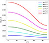 |
Fig. 1. Ratio Qeq(ω, i) = TIRFM/Teffeq as a function of the rotation axis inclination i on the line of sight, for various rotation rates ω between 0.2 and 0.7. The thickness of the lines represents the effects of mass and Xcore/Xenv variations in the intervals [2.0,2.4] and [0.25,0.45], respectively. |
Among all the grid models, acceptable models were identified using the following algorithm: for the model under investigation, we derived an interval of inclinations, imod, from its equatorial velocity, veqmod, such that veqmod sin imod and the observed v sin i were consistent within the uncertainties. We then defined the interval of model apparent luminosities corresponding to this inclination interval. If the so-computed interval of apparent luminosity had a non-void overlap with the observed one, the current model was tagged as matching this observable. A similar procedure was performed with the other observables (TIRFM, c′1, and c2). If the current model was tagged as matching all the observables, we selected it as a valid solution and moved on to the next one of the grid. Since the two stars at hand have also been observed with infrared interferometers (Zhao et al. 2009; Baines et al. 2018, 2025), we also carried out an additional test considering the equatorial radius to see how the set of solution changed when this additional constraint is taken into account.
3. Rasalhague – α Oph
3.1. Observational constraints
The first constraint we used is the apparent luminosity. From the bolometric flux fbol = 3.88 ± 0.19 × 10⁻⁹ W/m2 (Baines et al. 2018) and the distance d = 14.80 ± 0.13 pc (Gardner et al. 2021), we derived an apparent luminosity of Lapp = 26.6 ± 1.8 L⊙, which is consistent with previous values (e.g. Lapp = 25.6 L⊙; Monnier et al. 2010).
The next quantity was the projected equatorial velocity v sin i. We derived it from a series of 112 high-resolution spectra collected on 2024, June 4 (e.g. Rieutord et al. 2025) with the Neo-Narval spectrograph (Böhm et al. 2016) attached to the 2-metre Bernard Lyot telescope at Pic du Midi. A mean line profile was obtained with the least-squares deconvolution method (LSD; Donati et al. 1997) applied to the observed spectra. The typical signal-to-noise ratio is ∼15 000 per resolved element. By fitting a synthetic, rotationally broadened line profile, we were able to derive a precise value, namely v sin i = 224.3 ± 2.6 km/s. In Fig. 2, we show the median line profile and its fit. Uncertainty was estimated with different statistical methods such as bootstrapping and Monte Carlo methods. We did not take into account the possible effects of micro- or macro-turbulence on the line profile. To our knowledge, there is no measurement of these parameters for Rasalhague. However, noting the similarity of this star with Vega (see conclusions), and using Vega’s macro-turbulence estimate by Hill et al. (2010), we find a possible contribution of macro-turbulence on line profile of ∼0.1 km/s, which is negligible compared to present uncertainties. Finally, we point out that this line profile clearly shows the presence of the secondary4 of the Rasalhague system as the little dip near the bottom of the line and redshifted by its relative radial velocity of ∼ + 14 km/s. At the time of the observations, the orbital phase of the binary was near 0.4, implying a radial velocity of ∼ + 15.6 km/s according to Gardner et al. (2021)’s Fig. 3, which squares with our measure.
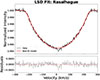 |
Fig. 2. Mean line profile of Rasalhague obtained with the least-squares deconvolution method (Donati et al. 1997) with a rotationally broadened profile fit to the data (top panel), and its residuals (bottom panel). The resulting projected equatorial velocity is 224.3 ± 2.6 km/s. |
The remaining constraints TIRFM, c′1, and c2 were derived from spectrophotometry, with spectra of Burnashev (1985) obtained through the VizieR service (Ochsenbein et al. 2000). Fluxes were provided for wavelengths between 320 and about 760 nm. Among the various spectra, we chose #1401, whose Strömgren c1 index (equal to 1.015) was closest to the value of Paunzen (2015), namely 1.039. This index was computed from each spectrum with a Python-translated adaptation of the Kurucz (1993) codes calibrated with the CALSPEC5 (e.g. Bohlin et al. 2014; Bohlin & Lockwood 2022) spectrum of Vega. To compute the three previously defined observables, we needed to know the flux farther than 320 nm in the UV domain and farther than 760 nm in the near-infrared domain. We completed the UV part of the spectrum with International Ultraviolet Explorer (IUE; Boggess et al. 1978) data obtained through the MAST archive6. From the so-called long-wavelength IUE data, we selected the three large aperture spectra that contained no negative flux values (LWR12747LL, LWR14250LL, and LWR14482LL). We then considered an average flux obtained with a mean weighted by the square root of the exposure time. For the infrared side, which is needed for computing TIRFM, we used a synthetic spectrum based on the ESTER model that matched best the data of Monnier et al. (2010), setting the inclination to i = 90°.
Each extension was scaled so as to ensure continuity with the Burnashev (1985) spectra, the mean IUE spectrum being degraded to the resolution of the spectrophotometric data beforehand. The scaling factor of the IUE part was of the same order of magnitude as the calibration correction proposed by Bohlin & Bianchi (2018). We ended up with the spectrum plotted in Fig. 3, from which we computed the observables displayed in Table 17. We used a conservative value of 5% for the flux uncertainties (Glushneva et al. 1992), which translated into 0.11 mag for the c′1 and c2 indices, of the same order of magnitude as that of typical c1 photometric measurements (Crawford & Barnes 1970). This systematic error was combined with the dispersion between the IUE spectra to yield the global uncertainty reported in Table 1.
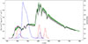 |
Fig. 3. Combined spectra of Rasalhague. The spectrophotometric part #1401 is shown by the solid black line. Its extension towards the UV is in magenta. The 5% uncertainty of these data is shown by the grey zone around the spectrum. The bandpasses of the filters used in the c′1 and c2 indices are shown in red and blue, respectively. The infrared extension is not shown. The green line shows the synthetic spectrum derived from the concordance model given in Table 3. The green zone around this line shows the effect of uncertainties of the rotation axis inclination. |
Observational constraints for Rasalhague.
3.2. Fundamental parameters of Rasalhague
As explained in Sect. 2.2, from a grid of 8162 models, we selected those matching the foregoing observational constraints. The parameters of the grid models were set around the values of the initial ESTER model that best matched the previous estimates by Monnier et al. (2010), as reported in Table 2. We thus scanned a mass range from 2.16 to 2.275 M⊙, a rotation rate from 0.55 to 0.7, and a relative hydrogen mass fraction in the core, Xc from 0.3 to 0.4. The mass fraction of hydrogen in the envelope Xenv was fixed to the initial solar one, X = 0.72 (e.g. Asplund et al. 2009), which seems reasonable for a star much younger than the Sun. The metallicity was computed from the relative abundances of Erspamer & North (2003), using solar abundances of Grevesse & Sauval (1998), thus yielding Z = 0.019.
Parameters of the initial ESTER model of Rasalhague.
In Fig. 4 we show the histograms of the parameters when either only the five observables Lapp, v sin i, TIRFM, c′1, and c2 were used, or when the interferometric measure of Req from Monnier et al. (2010) was added. Quite remarkably, the spectrophotometric equatorial radius agreed well with the interferometric value. The error bar on the interferometric value is, however, much lower, as expected. However, the added value of the spectrophotometric method is the determination of the rotation axis inclination on the line of sight. Zhao et al. (2009) could not determine this parameter properly as it turned out to be degenerate with the gravity-darkening exponent8β. Because of this degeneracy, Zhao et al. (2009) reverted to β = 0.25, the value derived by von Zeipel (1924), which is valid only for small rotation rates (Espinosa Lara & Rieutord 2011). This assumption led Zhao et al. (2009) to impose an inclination of 88.5°, which was slightly revised to 87.5° by Monnier et al. (2010), but still much larger than ours. Our result also squares with the polarimetric observations of Rasalhague by Bailey et al. (2020), who found the star inclination to be necessarily larger than 60°.
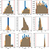 |
Fig. 4. Histograms of the distributions of mass, M; rotation rate with respect to the critical one, Ω/Ωc(=ω); equatorial radius, Req; relative hydrogen mass fraction in the core, Xc; inclination of the rotation axis, i; apparent luminosity, Lapp; and spectroscopic quantities, TIRFM, c′1, and c2. The blue histograms show the distribution when the interferometric constraint on Req from Monnier et al. (2010) is used, while the superimposed orange ones show the distributions when no interferometric constraint is used. Red lines on mass, Ω/Ωc, and Xc show the interval of the parameter that was scanned. Dashed red lines on the observed parameters show the constraints that had to be matched. |
Besides this, Rasalhague belongs to a binary system, and Gardner et al. (2021) measured an orbital plane inclination of 130.679 ± 0.067° with respect to the line of sight. Because spectroscopy and interferometry are blind in the direction of Rasalhague’s rotation, our results indicate that the spin vector can be oriented either at 70 or 110° with respect the line of sight. Consequently, the mutual orientation of the orbital and spin angular momenta are either 20 or 60° apart. Hence, according to present data, it seems difficult to assess that the two angular-momentum vectors are aligned, but the histograms in Fig. 4 show it is possible that they are just 5–10° apart.
To take the best of spectrophotometric and interferometric measurements, we also ran our model selection with spectrophotometric constraints together with the bounds on the equatorial radius given by Monnier et al. (2010). As shown in Fig. 4, the distributions were marginally altered, except that of Req of course. They also showed that the two photometric indices, c′1 and c2, do not play a role in the selection of the models in the present case. As a side note, we also remark that the histograms show that some models are outside the uncertainty interval of observed parameters. This is typical of models for which a change of inclination, within its uncertainties, put them in the observed range.
For the sake of completeness, we also used the radius determination of Baines et al. (2018), which was derived with the limb-darkened disc model. The resulting new distributions (not shown) presented only slight differences with those displayed in Fig. 4. In particular, the average inclination remained close to 70°.
We summarise our results concerning Rasalhague in Fig. 5, which shows that the models converge to a rather well-defined set of fundamental parameters. In Table 3, we gather all the values derived from our analysis with their error bars. Our mass agrees rather well with the value of Gardner et al. (2021), 2.20 ± 0.06 M⊙, which is a dynamical mass derived from the orbit of Rasalhague’s companion. We used the mass; the rotation rate, ω; and the ratio, Xc = Xcore/Xenv to design a new ESTER model, which is our concordance model for Rasalhague. In the same table we also report the values found by Monnier et al. (2010), which used a Roche model for determination. The results are quite close to ours, except for the effective temperatures, likely because of the discrepancy in the inclination. In this table we also report the polar and equatorial rotation periods. This is an output of the model, which includes the baroclinicity of the radiative envelope leading to the differential rotation of the star. It gives an idea of the expected surface differential rotation of Rasalhague.
 |
Fig. 5. Diagrams summarising the histograms of Fig. 4 when no constraint on the equatorial radius is applied (NC line) or when models meeting the equatorial radius of Monnier et al. (2010) are selected (M10 line). The red dots show the mean value and the segments the standard deviation. Green columns highlight the common values. |
Top: Most probable parameters of Rasalhague with 2D-ESTER models using the interferometric constraint on equatorial radius by Monnier et al. (2010). Bottom: 2D-ESTER concordance model of Rasalhague that fits all the observed quantities. The M10 column shows values derived by Monnier et al. (2010).
As a final touch, we computed a synthetic spectrum of Rasalhague based on the parameters of Table 3. This spectrum is plotted along the observed one in Fig. 3. Lines have been thickened with a grey or green over-line in order to show the uncertainties of both the observed and synthetic spectra. For the synthetic spectrum we just considered the effect of inclination error bar. We see that the observed SED and the synthetic one match fairly well.
To be thorough, we also wished to provide an estimate of the age of Rasalhague. To this end, we ran 1D evolving models until Xc reached a value of 0.361. We run the CESAM2k20 (Manchon et al. 2025), the Toulouse-Geneva evolution codes (Hui-Bon-Hoa 2008) and the Modules for Experiments in Stellar Astrophysics (Paxton et al. 2011, 2013, 2015, 2018; Jermyn et al. 2023). They all give an age around 600 Myr past the zero-age main sequence (ZAMS), in agreement with the previous estimate of Monnier et al. (2010), which used another 1D evolution code, namely Y2 of Demarque et al. (2004). However, the foregoing age was obtained with models neglecting any ‘turbulent’ diffusion. When such a diffusion is included, the convective core is fuelled with fresh hydrogen and takes more time to reach a given Xc. Some tests showed us that the increase can be significant, namely a few tens of percent. We thus conclude that 600 Myr is certainly a lower limit to the real age of Rasalhague. Hence, the precise estimate of the age of this star will have to wait for 2D models including turbulent transport to be operational9.
4. Alkaid – η UMa
4.1. Observational constraints
We used the CALSPEC spectrum10 of Alkaid to derive the observables we needed: c′1 = −0.927 ± 0.07, c2 = 5.995 ± 0.07, and TIRFM = 16781 ± 100 K. The uncertainties were determined from the flux accuracy in each part of the spectrum. We determined the bolometric flux of Alkaid on Earth by integration of the CALSPEC spectrum and using the HIPPARCOS parallax, from which we found a distance of 31.38 ± 0.24 pc. The subsequent apparent luminosity was equal to Lapp = 583 ± 30 L⊙, which is in agreement with the value of 594 ± 31 L⊙ from Baines et al. (2018). We did not consider the revised values of Baines et al. (2025) because of the much lower effective temperature (13946 ± 60 K) they obtained, which is inconsistent with the values we derived from CALSPEC data.
The value of v sin i was computed the same way as for Rasalhague, but with spectra extracted from PolarBase11, a database for high-resolution spectropolarimetric data (Petit et al. 2014). We extracted 52 spectra collected on 2015, March 12, with the Narval spectropolarimeter (Aurière 2003). The signal-to-noise ratio of the resulting LSD profile is ∼2500 per resolved element. The best fit yielded v sin i = 154.3 ± 9.1 km.s−1. In Fig. 6 we show the actual line profile and its adjustment by a rotationally broadened absorption line. These observational constraints are gathered in Table 4.
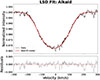 |
Fig. 6. Mean line profile of Alkaid obtained with the least-squares deconvolution method with a rotationally broadened profile fit to the data (top panel), and its residuals (bottom panel). The resulting projected velocity is 154.3 ± 9.1 km/s. |
Observational constraints for Alkaid.
4.2. Parameters derived from the models
To start our grid of models we first observed that the apparent luminosity of Alkaid could be reproduced by a ZAMS non-rotating 5.1 M⊙ ESTER model (L = 583 L⊙) with Xenv = 0.7 and Z = 0.02. We kept this chemical composition throughout the analysis of Alkaid. Its radius of 2.65 R⊙ combined with a minimum equatorial velocity equal to the observed V sin i gave a minimum value of ω ∼ 0.28. Assuming that the star is young, we therefore scanned the following parameter space: 4.98 ≤ M/M⊙ ≤ 5.20, 0.2 ≤ ω ≤ 0.6, and 0.8 ≤ Xc ≤ 1, where we distributed about 5100 models.
We then selected models matching the observational constraints as for Rasalhague, but no measure of equatorial radius was used here. Some interferometric measurements of the angular diameter were taken by Baines et al. (2018, 2025), Gordon et al. (2019) and Abe et al. (2024), but these works turned out to be too imprecise to be useful to the selection of models.
The parameter and observable histograms for Alkaid are displayed in Fig. 7. As shown by the red lines on the scanned parameters (M, Ω/Ωc, and Xc), the grid was wide enough not to miss any possible model. Clearly, the four observables Lapp, TIRFM, c′1, and c2 played a role in the selection of models, and the most probable parameters were clearly emerging. In Table 5 we show all the parameters we determined, along with those of the concordance ESTER model. The proxy of the age, Xc, points to 0.97, meaning that Alkaid is barely off the ZAMS. To give a figure for the age, we ran a time-evolving 2D model with the ESTER code. We plot the evolutionary track of the star in the (TIRFM, Lapp) plane in Fig. 8, which shows that Alkaid evolved for  Myr after the ZAMS.
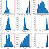 |
Fig. 7. Histograms of parameter distributions of steady 2D-ESTER models for Alkaid that match the observational constraints. Red lines have the same meaning as in Fig. 4. |
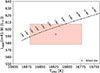 |
Fig. 8. Evolutionary track in a Hertzsprung–Russell-like diagram showing the evolution the best ESTER Alkaid model during the first 12 Myr on the main sequence. The red cross represents the mean observed value, and its uncertainty box is depicted by the pink area. |
Top: Most probable parameters of Alkaid with steady 2D-ESTER models. Bottom: 2D-ESTER concordance model of Alkaid that fits all the observed quantities.
From the foregoing results and the distance to this star we were also able to infer its equatorial angular diameter, which we find equal to 0.844 ± 0.009 mas (uncertainty comes from that of the distance). This value is consistent with 0.981 ± 0.144 mas of Baines et al. (2018), with θLD = 0.834 ± 0.06 mas of Gordon et al. (2019) and with θLD = 0.828 ± 0.029 mas of Abe et al. (2024). These latter measurements were obtained with interferometry (intensity interferometer for Abe et al. 2024) and do not distinguish between polar and equatorial radii. If we assume that they measure the radius of a disc of surface equal to the projected surface of the star on the sky, our model says that the angular diameter of that disc would be 0.826 ± 0.006 mas, which is still in line with the foregoing observations.
5. Conclusions
We show that the fundamental parameters of early-type, fast-rotating stars can be derived from high-quality spectrophotometric data and high-resolution, high-signal-to-noise ratio spectroscopy. In addition, we were able to determine the inclination of their rotation axis on the line of sight. This was possible thanks to gravity darkening, which makes the characteristics of the SED dependent on the orientation of the rotation axis and on the rotational flattening. This allowed us to infer the parameters for two stars: Rasalhague (α Oph) and Alkaid (η UMa). For the first star we were able derive the true orientation of its rotation axis, a quantity that escaped the interferometric measurements because of a degeneracy between this angle and the so-called gravity darkening exponent (Zhao et al. 2009; Monnier et al. 2010). The choice of Alkaid was directed by the availability of a complete SED from CALSPEC, that is, well-calibrated data from space instruments covering the spectral interval from the ultraviolet to the near-infrared domains. This star, of spectral type B3V, also offered a test of our method for the case of hot stars.
For now, our method uses spectrophotometric data, because fluxes in the UV bands we defined are not available. Should some UV photometry with bands near those we used become available in the future, the method would only require the different magnitudes in the filters used to compute the c1′ and c2 indices. As for TIRFM, we would compute it from an infrared flux and the bolometric flux. The case of stars far enough for reddening to be considered could thus be treated, provided we have de-reddening laws for the c1′ and c2 indices, as they exist for the uvbyβ system.
Of course, one has to keep in mind that our method has its limits: (i) it only works if the gravity darkening is strong enough, that is, if rotation is fast enough. The actual limit is not known, but we estimate it at 30% of the critical angular velocity; this is a value that has to be checked; (ii) we need data in the UV bands (i.e. from space); and (iii) the parameters we derived represent an element of a set of ESTER models. Obviously, if we change the physics or some assumed inputs of the models, the parameters we derive are likely to change. For instance, the chemical composition was assumed and fixed. For our method to provide realistic results, we need at least some clues about the actual composition.
The positive side of these results is that we now know these two stars better. Concerning Rasalhague, we confirm the results Monnier et al. (2010) obtained with interferometry and seismology, and we complete them by giving the inclination of its rotation axis on the line of sight (69 ± 6°). Such an inclination, together with rotation, could also be constrained by linear polarisation measurements such as Regulus (α Leo), as worked out by Cotton et al. (2017), but see also Bailey et al. (2020).
We note that Rasalhague is quite similar to Vega in terms of mass and age, but its spectral type A5IV, instead of A0V for Vega, essentially reflects its nearly equatorial view compared to the nearly polar-on view of Vega. This result shows that the determination of the spin axis orientation is essential for rapidly rotating stars, when one interprets the spectral type in terms of evolutionary status. With Rasalhague and Vega we have an example where the former is younger than the latter, although of later spectral type (and higher luminosity class).
The case of Alkaid showed that our method also works on such hot, intermediate-mass stars. We learned that it is a very young star, typically 6 Myr beyond the ZAMS, with a mass ∼5.07 M⊙.
An interesting consequence of knowing (or better knowing) the inclination of the rotation axis on the line of sight is that we can now determine the visibility of the oscillation modes of these two stars. Rasalhague is well known as a δ-Scuti oscillator, with a rich oscillation spectrum (Monnier et al. 2010), while Alkaid also shows oscillations (Rudrasingam et al. 2026), the spectrum of which displays a peak at a period of about 14.1 h, which could be associated with the rotation period of this star, since we find it at Prot = 14.6 ± 1.9 h.
A natural follow up to this work will involve refinements of the proposed models of these two stars, taking into account the seismological constraints from the TESS satellite as was done with Altair (Bouchaud et al. 2020; Rieutord et al. 2024). This will be presented in a future work.
Acknowledgments
We are very grateful to the referee for many valuable comments, which helped us improve the original manuscript. The research leading to these results has received funding from the European Research Council (ERC) under the Horizon Europe programme (Synergy Grant agreement N°101071505: 4D-STAR). While partially funded by the European Union, views and opinions expressed are however those of the authors only and do not necessarily reflect those of the European Union or the European Research Council. Neither the European Union nor the granting authority can be held responsible for them. Most of the calculations have been performed on CALMIP supercomputing center (Grant 2023-P20025). This research made also use of the VizieR catalogue access tool, CDS, Strasbourg, France (DOI : 10.26093/cds/vizier).
References
- Abe, S., Abhir, J., Acciari, V. A., et al. 2024, MNRAS, 529, 4387 [CrossRef] [Google Scholar]
- Abt, H. A., & Morrell, N. I. 1995, ApJS, 99, 135 [Google Scholar]
- Asplund, M., Grevesse, N., Sauval, A. J., & Scott, P. 2009, Ann. Rev. Astron. Astrophys., 47, 481 [CrossRef] [Google Scholar]
- Aurière, M. 2003, EAS Publ. Ser., 9, 105 [CrossRef] [EDP Sciences] [Google Scholar]
- Bailey, J., Cotton, D. V., Howarth, I. D., Lewis, F., & Kedziora-Chudczer, L. 2020, MNRAS, 494, 2254 [NASA ADS] [CrossRef] [Google Scholar]
- Baines, E. K., Armstrong, J. T., Schmitt, H. R., et al. 2018, AJ, 155, 30 [Google Scholar]
- Baines, E. K., Clark, J. H., Kingsley, B. I., Schmitt, H. R., & Stone, J. M. 2025, AJ, 169, 293 [Google Scholar]
- Blackwell, D. E., Petford, A. D., & Shallis, M. J. 1980, A&A, 82, 249 [NASA ADS] [Google Scholar]
- Boggess, A., Carr, F. A., Evans, D. C., et al. 1978, Nature, 275, 372 [NASA ADS] [CrossRef] [Google Scholar]
- Bohlin, R. C., & Bianchi, L. 2018, AJ, 155, 162 [Google Scholar]
- Bohlin, R. C., & Lockwood, S. 2022, Update of the STIS CTE Correction Formula for Stellar Spectra, Instrument Science Report STIS 2022–7 [Google Scholar]
- Bohlin, R. C., Gordon, K. D., & Tremblay, P. E. 2014, PASP, 126, 711 [NASA ADS] [Google Scholar]
- Böhm, T., Cabanac, R., & Lopez-Ariste, A. 2016, Technical Specifications, Tech. rep., Obs. Midi-Pyrénées [Google Scholar]
- Bouchaud, K., Domiciano de Souza, A., Rieutord, M., Reese, D. R., & Kervella, P. 2020, A&A, 633, A78 [NASA ADS] [CrossRef] [EDP Sciences] [Google Scholar]
- Burnashev, V. I. 1985, Abastumanskaia Astrofizicheskaia Observatoriia Byulleten, 59, 83 [NASA ADS] [Google Scholar]
- Burssens, S., Bowman, D. M., Michielsen, M., et al. 2023, Nat. Astron., 7, 913 [NASA ADS] [CrossRef] [Google Scholar]
- Cotton, D. V., Bailey, J., Howarth, I. D., et al. 2017, Nat. Astron., 1, 690 [Google Scholar]
- Crawford, D. L., & Barnes, J. V. 1970, AJ, 75, 978 [NASA ADS] [CrossRef] [Google Scholar]
- Demarque, P., Woo, J.-H., Kim, Y.-C., & Yi, S. K. 2004, ApJS, 155, 667 [NASA ADS] [CrossRef] [Google Scholar]
- Donati, J. F., Semel, M., Carter, B. D., Rees, D. E., & Collier Cameron, A. 1997, MNRAS, 291, 658 [Google Scholar]
- Erspamer, D., & North, P. 2003, A&A, 398, 1121 [NASA ADS] [CrossRef] [EDP Sciences] [Google Scholar]
- Espinosa Lara, F., & Rieutord, M. 2011, A&A, 533, A43 [NASA ADS] [CrossRef] [EDP Sciences] [Google Scholar]
- Espinosa Lara, F., & Rieutord, M. 2013, A&A, 552, A35 [NASA ADS] [CrossRef] [EDP Sciences] [Google Scholar]
- Gardner, T., Monnier, J. D., Fekel, F. C., et al. 2021, ApJ, 921, 41 [Google Scholar]
- Glushneva, I. N., Kharitonov, A. V., Kniazeva, L. N., & Shenavrin, V. I. 1992, ApJS, 92, 1 [Google Scholar]
- Gordon, K. D., Gies, D. R., Schaefer, G. H., Huber, D., & Ireland, M. 2019, ApJ, 873, 91 [NASA ADS] [CrossRef] [Google Scholar]
- Gray, R. O., Napier, M. G., & Winkler, L. I. 2001, AJ, 121, 2148 [Google Scholar]
- Grevesse, N., & Sauval, A. J. 1998, Space Sci. Rev., 85, 161 [Google Scholar]
- Hauschildt, P. H., Allard, F., & Baron, E. 1999, ApJ, 512, 377 [Google Scholar]
- Hill, G., Gulliver, A. F., & Adelman, S. J. 2010, ApJ, 712, 250 [NASA ADS] [CrossRef] [Google Scholar]
- Hui-Bon-Hoa, A. 2008, Ast. Space Sc., 316, 55 [Google Scholar]
- Jermyn, A. S., Bauer, E. B., Schwab, J., et al. 2023, ApJS, 265, 15 [NASA ADS] [CrossRef] [Google Scholar]
- Kurucz, R. 1993, ATLAS9 Stellar Atmosphere Programs and 2 km/s grid. Kurucz CD-ROM No. 13. Cambridge, 13 [Google Scholar]
- Lazzarotto, A., Hui-Bon-Hoa, A., & Rieutord, M. 2023, A&A, 676, A50 [NASA ADS] [CrossRef] [EDP Sciences] [Google Scholar]
- Manchon, L., Deal, M., Marques, J. P. C., & Lebreton, Y. 2025, A&A, 704, A79 [Google Scholar]
- Mombarg, J. S. G., Dotter, A., Rieutord, M., et al. 2022, ApJ, 925, 154 [NASA ADS] [CrossRef] [Google Scholar]
- Mombarg, J. S. G., Rieutord, M., & Espinosa Lara, F. 2023, A&A, 677, L5 [NASA ADS] [CrossRef] [EDP Sciences] [Google Scholar]
- Monnier, J. D., Townsend, R. H. D., Che, X., et al. 2010, ApJ, 725, 1192 [NASA ADS] [CrossRef] [Google Scholar]
- Monnier, J., Che, X., Zhao, M., et al. 2012, ApJ, 761, L3 [NASA ADS] [CrossRef] [Google Scholar]
- Negueruela, I., Simón-Díaz, S., de Burgos, A., Casasbuenas, A., & Beck, P. G. 2024, A&A, 690, A176 [NASA ADS] [CrossRef] [EDP Sciences] [Google Scholar]
- Ochsenbein, F., Bauer, P., & Marcout, J. 2000, A&AS, 143, 23 [NASA ADS] [CrossRef] [EDP Sciences] [Google Scholar]
- Paunzen, E. 2015, A&A, 580, A23 [NASA ADS] [CrossRef] [EDP Sciences] [Google Scholar]
- Paxton, B., Bildsten, L., Dotter, A., et al. 2011, ApJS, 192, 3 [Google Scholar]
- Paxton, B., Cantiello, M., Arras, P., et al. 2013, ApJS, 208, 4 [Google Scholar]
- Paxton, B., Marchant, P., Schwab, J., et al. 2015, ApJS, 220, 15 [Google Scholar]
- Paxton, B., Schwab, J., Bauer, E. B., et al. 2018, ApJS, 234, 34 [NASA ADS] [CrossRef] [Google Scholar]
- Petit, P., Louge, T., Théado, S., et al. 2014, PASP, 126, 469 [NASA ADS] [CrossRef] [Google Scholar]
- Rieutord, M., Espinosa Lara, F., & Putigny, B. 2016, J. Comp. Phys., 318, 277 [NASA ADS] [CrossRef] [Google Scholar]
- Rieutord, M., Reese, D. R., Mombarg, J. S. G., & Charpinet, S. 2024, A&A, 687, A259 [NASA ADS] [CrossRef] [EDP Sciences] [Google Scholar]
- Rieutord, M., Böhm, T., Domiciano de Souza, A., et al. 2025, in SF2A-2025: Proceedings of the Annual meeting of the French Society of Astronomy and Astrophysics, eds. A. Siebert, K. Baillié, M. Béthermin, et al., 403 [Google Scholar]
- Rudrasingam, J., Bedding, T. R., Pope, B. J. S., et al. 2026, MNRAS, 547, 413 [Google Scholar]
- Strömgren, B. 1963, Q. J. R. Astron. Soc., 4, 8 [Google Scholar]
- von Zeipel, H. 1924, MNRAS, 84, 665 [NASA ADS] [CrossRef] [Google Scholar]
- Zhao, M., Monnier, J. D., Pedretti, E., et al. 2009, ApJ, 701, 209 [NASA ADS] [CrossRef] [Google Scholar]
- Zorec, J., & Royer, F. 2012, A&A, 537, A120 [NASA ADS] [CrossRef] [EDP Sciences] [Google Scholar]
Evolution STEllaire en Rotation.
If not stated otherwise, Rasalhague refers to the primary of this binary system (e.g. Gardner et al. 2021).
The code is publicly available at https://ester-project.github.io/ester
The best description of this star is given in Gardner et al. (2021), which gave a mass for the secondary equal to 0.824 ± 0.023 M⊙. At the age of Rasalhague (∼600 Myr), such a mass implies an effective temperature of 4750 K and a luminosity of 0.25 L⊙ according to CESAM2k20 models (Manchon et al. 2025).
Note that in Fig. 15 of Lazzarotto et al. (2023) the plotted bandpass profile of the F220 filter was erroneously given as that of the ACS_HRC.F220W instead of that of the HSP_UV1_F220W_A, which we used in both works.
A simplified model of gravity darkening assumes that the latitudinal variations of effective temperature follow the latitudinal variations of the effective gravity as Teff ∝ geffβ. However, Espinosa Lara & Rieutord (2011) showed that β depends on the rotation rate of the star.
The 2D-ESTER evolution code faces numerical difficulties in the mass range of Rasalhague.
The file is etauma_stis_008.fits.
All Tables
Top: Most probable parameters of Rasalhague with 2D-ESTER models using the interferometric constraint on equatorial radius by Monnier et al. (2010). Bottom: 2D-ESTER concordance model of Rasalhague that fits all the observed quantities. The M10 column shows values derived by Monnier et al. (2010).
Top: Most probable parameters of Alkaid with steady 2D-ESTER models. Bottom: 2D-ESTER concordance model of Alkaid that fits all the observed quantities.
All Figures
|
Fig. 1. Ratio Qeq(ω, i) = TIRFM/Teffeq as a function of the rotation axis inclination i on the line of sight, for various rotation rates ω between 0.2 and 0.7. The thickness of the lines represents the effects of mass and Xcore/Xenv variations in the intervals [2.0,2.4] and [0.25,0.45], respectively. |
| In the text | |
|
Fig. 2. Mean line profile of Rasalhague obtained with the least-squares deconvolution method (Donati et al. 1997) with a rotationally broadened profile fit to the data (top panel), and its residuals (bottom panel). The resulting projected equatorial velocity is 224.3 ± 2.6 km/s. |
| In the text | |
|
Fig. 3. Combined spectra of Rasalhague. The spectrophotometric part #1401 is shown by the solid black line. Its extension towards the UV is in magenta. The 5% uncertainty of these data is shown by the grey zone around the spectrum. The bandpasses of the filters used in the c′1 and c2 indices are shown in red and blue, respectively. The infrared extension is not shown. The green line shows the synthetic spectrum derived from the concordance model given in Table 3. The green zone around this line shows the effect of uncertainties of the rotation axis inclination. |
| In the text | |
|
Fig. 4. Histograms of the distributions of mass, M; rotation rate with respect to the critical one, Ω/Ωc(=ω); equatorial radius, Req; relative hydrogen mass fraction in the core, Xc; inclination of the rotation axis, i; apparent luminosity, Lapp; and spectroscopic quantities, TIRFM, c′1, and c2. The blue histograms show the distribution when the interferometric constraint on Req from Monnier et al. (2010) is used, while the superimposed orange ones show the distributions when no interferometric constraint is used. Red lines on mass, Ω/Ωc, and Xc show the interval of the parameter that was scanned. Dashed red lines on the observed parameters show the constraints that had to be matched. |
| In the text | |
|
Fig. 5. Diagrams summarising the histograms of Fig. 4 when no constraint on the equatorial radius is applied (NC line) or when models meeting the equatorial radius of Monnier et al. (2010) are selected (M10 line). The red dots show the mean value and the segments the standard deviation. Green columns highlight the common values. |
| In the text | |
|
Fig. 6. Mean line profile of Alkaid obtained with the least-squares deconvolution method with a rotationally broadened profile fit to the data (top panel), and its residuals (bottom panel). The resulting projected velocity is 154.3 ± 9.1 km/s. |
| In the text | |
|
Fig. 7. Histograms of parameter distributions of steady 2D-ESTER models for Alkaid that match the observational constraints. Red lines have the same meaning as in Fig. 4. |
| In the text | |
|
Fig. 8. Evolutionary track in a Hertzsprung–Russell-like diagram showing the evolution the best ESTER Alkaid model during the first 12 Myr on the main sequence. The red cross represents the mean observed value, and its uncertainty box is depicted by the pink area. |
| In the text | |
Current usage metrics show cumulative count of Article Views (full-text article views including HTML views, PDF and ePub downloads, according to the available data) and Abstracts Views on Vision4Press platform.
Data correspond to usage on the plateform after 2015. The current usage metrics is available 48-96 hours after online publication and is updated daily on week days.
Initial download of the metrics may take a while.