


| Issue |
A&A
Volume 710, June 2026
|
|
|---|---|---|
| Article Number | A328 | |
| Number of page(s) | 11 | |
| Section | Planets, planetary systems, and small bodies | |
| DOI | https://doi.org/10.1051/0004-6361/202659005 | |
| Published online | 25 June 2026 | |
The spectral energy distribution of YSES 1 b and its circumplanetary disc★
1
SRON – Space Research Organisation Netherlands,
Niels Bohrweg 4,
2333
CA
Leiden,
The Netherlands
2
Leiden Observatory, Leiden University,
PO Box 9513,
2300
RA
Leiden,
The Netherlands
3
Steward Observatory, The University of Arizona,
933 North Cherry Avenue,
Tucson,
AZ,
USA
4
Subaru Telescope, National Observatory of Japan, NINS,
650 N. A’ohoku Place,
Hilo,
HI,
USA
5
Wyant College of Optical Sciences, The University of Arizona,
1630 E University Boulevard,
Tucson,
AZ,
USA
6
Astrobiology Center, National Institutes of Natural Sciences,
2-21-1 Osawa, Mitaka,
Tokyo,
Japan
7
Northrop Grumman Corporation,
600 South Hicks Road,
Rolling Meadows,
IL,
USA
8
Center for Computational Astrophysics, Flatiron Institute,
162 5th Avenue,
New York,
NY,
USA
9
Draper Laboratory,
555 Technology Square,
Cambridge,
MA,
USA
10
Department of Astronomy, University of Michigan,
323 West Hall, 1085 S University Ave,
Ann Arbor,
MI
48109,
USA
11
Starfire Optical Range, Kirtland Air Force Base,
Albuquerque,
NM,
USA
★★ Corresponding author: This email address is being protected from spambots. You need JavaScript enabled to view it.
Received:
16
January
2026
Accepted:
24
April
2026
Abstract
Context. Direct imaging enables the characterisation of substellar companions on wide orbits. These objects provide a testbed for our formation theories; therefore, it is important to obtain accurate physical parameters for them. One of these objects is YSES 1 b.
Aims. Our objective is to improve the spectral energy distribution (SED) modelling of YSES 1 b and determine the bulk and atmospheric parameters.
Methods. We obtained observations in the r′, i′, and z′ bands using MagAO-X on the 6.5 metre Magellan Clay telescope at Las Campanas Observatory. We combined this data with archival VLT/SPHERE and VLT/NACO data and used a forward-modelling approach to estimate the physical parameters. We tested models both without and with a circumplanetary disc (CPD) model. We represented the CPD by including a dust extinction model and a blackbody radiation component. Using the derived bolometric luminosity, we estimated the mass of YSES 1 by fitting evolutionary models.
Results. Including the CPD model provides a significantly better fit to the photometric data, yielding an object that is considerably warmer (2854−94+110 K vs 1727−127+172 K) and smaller (1.58−0.07+0.06 RJ vs 3.0−0.7+0.2 RJ) than previous estimates. The newly determined radius suggests that the addition of dust extinction could resolve the large radius anomaly identified previously. Depending on the age of the system, the estimated mass increases from 14 ± 3 MJ (17 Myr) to either 25.7−3.6+4.1 (17 Myr) or 41.6−3.4+3.6 MJ (27 Myr).
Conclusions. Dust extinction and blackbody radiation from a CPD can substantially change the estimated physical parameters of an object. For YSES 1 b, this moves it into the brown dwarf regime.
Key words: instrumentation: high angular resolution / planets and satellites: atmospheres / planets and satellites: individual: YSES 1 b
This paper includes data gathered with the 6.5 meter Magellan Telescopes located at Las Campanas Observatory, Chile.
© The Authors 2026
 Open Access article, published by EDP Sciences, under the terms of the Creative Commons Attribution License (https://creativecommons.org/licenses/by/4.0), which permits unrestricted use, distribution, and reproduction in any medium, provided the original work is properly cited.
This article is published in open access under the Subscribe to Open model. This email address is being protected from spambots. You need JavaScript enabled to view it. to support open access publication.
1 Introduction
Direct imaging of exoplanets provides valuable information on planet formation and demographics. The sensitivity of current instrumentation enables the detection of young, giant, self-luminous planets on orbits with semi-major axes from tens to hundreds of AU, which is a population of objects almost exclusively accessible through direct imaging (Currie et al. 2023). Furthermore, because photons are detected directly from the objects themselves, atmospheric characterisation is possible, which improves our physical understanding of these companions.
One of the systems that provides an interesting test for our planet formation theories is YSES 1, a young solar-type star located in the Lower Centaurus Crux subgroup of the Scorpius-Centaurus association (Pecaut & Mamajek 2016). Two substellar-companions (YSES 1 b and c) are known to orbit at projected separations of 160 AU and 320 AU (Bohn et al. 2020a,b). Initial spectral energy distribution (SED) fits using photometric data from 1–5 μm provided mass estimates of 14 ± 3 MJ and 6 ± 1 MJ respectively.
Since its discovery, YSES 1 b has received considerable observational follow-up. Abundance ratios have been measured to investigate the formation history. Zhang et al. (2021) first measured the 12CO/13CO isotopologue ratio using medium-resolution K-band data from VLT/SINFONI and report an enriched value of ![Mathematical equation: $\[31_{-10}^{+17}\]$](/articles/aa/full_html/2026/06/aa59005-26/aa59005-26-eq7.png) . A subsequent analysis based on VLT/CRIRES+ observations provides a different value of 88 ± 13 (Zhang et al. 2024). Despite the discrepancy between the two retrieved 12CO/13CO ratios, both datasets suggest a solar-like C/O ratio. More recently, Roberts et al. (2025) constrained the orbit of YSES 1 b using archival astrometry, radial velocity data, proper motion measurements, and new VLTI/GRAVITY data. They find a moderate eccentricity of 0.44 ± 0.20, indicating a complex dynamical history. They also revise the semi-major axis to a slightly smaller value of
. A subsequent analysis based on VLT/CRIRES+ observations provides a different value of 88 ± 13 (Zhang et al. 2024). Despite the discrepancy between the two retrieved 12CO/13CO ratios, both datasets suggest a solar-like C/O ratio. More recently, Roberts et al. (2025) constrained the orbit of YSES 1 b using archival astrometry, radial velocity data, proper motion measurements, and new VLTI/GRAVITY data. They find a moderate eccentricity of 0.44 ± 0.20, indicating a complex dynamical history. They also revise the semi-major axis to a slightly smaller value of ![Mathematical equation: $\[146_{-10}^{+16}\]$](/articles/aa/full_html/2026/06/aa59005-26/aa59005-26-eq8.png) AU.
AU.
In addition to measuring abundance ratios, Zhang et al. (2021) detected emission from the Brackett γ line, suggesting that the companion is still accreting from a circumplanetary disc (CPD). Holstein et al. (2021) attempted to detect the CPD using polarimetric observations but only found an upper limit. Another possible inference of the existence of a CPD is the relatively low projected rotational velocity measured in Zhang et al. (2024), where magnetic braking from the CPD slows down the rotation. More substantial evidence for the CPD recently came from James Webb Space Telescope (JWST) spectroscopy (Hoch et al. 2025). Based on the infrared excess in the SED, the best fit results in a blackbody disc temperature of approximately 500 K and a disc radius between 8.5–20 RJ. They explain a broad emission feature at 8–11 μm by sub-micron olivine grains. Recently, Julo et al. (2025) used VLT/MUSE to measure the Hα, Hβ, CaII H&K triplet, and HeI emission lines associated with accretion. From the Hα line they estimated an accretion rate of ~1.45 × 10⁻⁹±0.19 MJ/year. These findings place YSES 1 b within a small group of known substellar companions that host a CPD. Other notable objects include GQ Lup b (Stolker et al. 2021), PDS 70 c (Benisty et al. 2021; Haffert et al. 2019), GSC 6214-210 b (Bowler et al. 2011; Bailey et al. 2013; Bowler et al. 2015), DH Tau b (Zhou et al. 2014), CT Cha b (Cugno & Grant 2025), and Delorme 1 (AB) b (Betti et al. 2022; Demars et al. 2025).
In this paper, we extend the photometric data of YSES 1 b to the optical bands using observations from the MagAO-X instrument (Males et al. 2024). Together with archival photometric data, we update the SED modelling of YSES 1 b and its CPD by including dust extinction and a blackbody emission component. Section 2 presents the MagAO-X observations and the data reduction to retrieve the contrast and astrometry. Section 3 presents the results of our SED fits and mass estimates. Section 4 discusses the implications of these results. Section 5 presents the conclusions.
MagAO-X observations.
2 Observations
We observed the YSES 1 system using MagAO-X on the 6.5 metre Magellan Clay telescope at Las Campanas Observatory. The MagAO-X extreme adaptive optics instrument is designed for high-contrast imaging in the visible to near-infrared (Males et al. 2024; Close et al. 2018). It uses a pyramid wavefront sensor in combination with a woofer-tweeter deformable mirror (DM) setup for high-order wavefront control. It uses an additional DM for non-common-path correction. The science arm consists of two electron-multiplying CCDs (EMCCDs), camsci1 and camsci2, which perform simultaneous observations in two different filters1.
Table 1 summarises the observations performed on 7 March 2023. We acquired the observations in pupil-tracking mode to provide angular diversity, enabling the removal of diffraction from the central star (Marois et al. 2006). We did not use a coronagraph during the observations. We obtained data in three filters: r′, i′, and z′. We measured the i′ band with camsci1, while the r′ and z′ band were obtained with camsci2. In addition to the science data, we took a set of dark frames for both cameras.
We processed the MagAO-X observations using PynPoint version 0.11.0 (Stolker et al. 2019). The PynPoint package reduces high-contrast imaging datasets and uses principal component analysis (PCA) to subtract the point spread function (PSF) of the host star (Amara & Quanz 2012). We began the data reduction by subtracting the median dark frame. We then rescaled the images along the x-axis to account for the different plate scales of the x and y axes, following Table 4 in Long et al. (2025). We aligned and centred individual frames on the host star in a series of steps. First, we determined the stellar centre in each frame to pixel accuracy by locating the maximum value after smoothing it with a two-dimensional Gaussian kernel with full width at half maximum (FHWM) of 30 mas. Second, we registered the frames by cross-correlating each frame with a subset of randomly selected reference frames to determine the average offset and then resampled the frames using spline interpolation. Finally, we applied an additional shift to place the star in the centre of the frames. We removed frames with poor seeing conditions based on aperture photometry of the unsaturated host star PSF to produce the final dataset for angular differential imaging (ADI) processing. We discarded frames in which the host flux was lower than 3-sigma below the maximum measured flux. This led to 6,17 and 4 frames being removed in the r′, i′ and z′ bands, respectively.
We applied PCA to estimate the PSF of the host star in every frame. We subtracted the first PCA component and derotated the frames, taking into account rotation corrections of 1.53 and 1.50 degrees for camsci1 and camsci2, respectively, to orient north upwards (Long et al. 2025). We took the median values to produce the resulting images.
Figure 1 shows the final images for each filter. We applied an additional Gaussian smoothing with a 30 mas FWHM kernel to reduce the high-frequency noise left over from the PSF subtraction and to highlight the companion. We clearly detect YSES 1 b in the i′ and z′ filters with signal-to-noise ratio (S/N) of 13.0 and 11.2, respectively. We estimated the S/N by comparing the companion signal to the noise in an annulus at the same separation, which at these distances is assumed to have a normal distribution. We do not detect YSES 1 b in the r′ filter.
We obtained the photometry and astrometry of YSES 1 b in the i′ and z′ bands using the negative artificial planet injection technique implemented in PynPoint, in which we subtracted a template PSF at the approximate location of the companion in each frame to remove its signal in the post-processed image (Stolker et al. 2020). We then determined the contrast and position of the companion by scaling and moving the PSF template to minimise the residuals.
We estimated the companion PSF in each frame based on the host star PSF by selecting a region of 0.35 arcsec around the star. We then performed a simplex minimisation to determine a first estimate of the best-fit contrast and position. We used these values as initial conditions for a Markov chain Monte Carlo (MCMC) analysis to retrieve the posterior distributions of the parameters (MacKay 2003). We selected a total of 50 walkers and 2000 steps per walker for the sampling. We applied a burn-in of 120 samples and thinned the chain by selecting every 18th sample based on autocorrelation analysis. We show the posterior distributions in Appendix A. In addition to the MCMC estimates, we also analysed possible systematic errors using the injection of artificial planets as described in Stolker et al. (2020). Appendix B details the distributions for the contrast, separation, and position angle offsets. We produced the final contrast, separation, and position angle by adding the bias estimates and adding the uncertainties in quadrature. Table 2 provides a summary of the results for both the i′ and z′ filters. The separation and position angle are consistent with the GRAVITY measurements reported in Roberts et al. (2025).
Since there is no detection in the r′ filter, we approximated the flux as a Gaussian with zero mean and a standard deviation equal to the 1σ upper limit. Using artificial planet injection at the separation of YSES 1 b to estimate the amount of self-subtraction, we derive a 1σ magnitude-contrast upper limit of 12.24 mag.
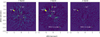 |
Fig. 1 Reduced MagAO-X images of the YSES 1 system in the r′, i′ and z′ filters after PCA-based PSF subtraction and Gaussian filtering. The point sources on the top are confirmed background stars (Bohn et al. 2020a). YSES 1 b is recovered in the i′ and z′ bands with an S/N of 13.0 and 11.2, respectively. |
3 Analysis
We revisited the physical modelling of YSES 1 b using a combination of the MagAO-X photometry obtained in Section 2 and archival SPHERE and NACO data (Bohn et al. 2020a). Here, we present the SED fitting and mass estimation.
3.1 Photometric calibration
Converting the derived contrasts in the MagAO-X filters to apparent magnitudes requires a flux calibration of the host star. To achieve this we performed an SED fit to existing photometric data. For the stellar atmosphere we employed the BT-Settl-CIFIST model (Allard 2013). We used the species package to estimate the posterior distributions of the model parameters using a nested-sampling approach (Stolker et al. 2020). Figure 2 shows the results. We used 17 photometric points from TYCHO (Høg et al. 2000), APASS (Henden et al. 2016), GAIA (Gaia Collaboration 2023), DENIS (Epchtein et al. 1999), 2MASS (Cutri et al. 2003) and WISE (Cutri et al. 2012). We set the distance of the system to 94.067 ± 0.105 (pc) (Bailer-Jones et al. 2021). An initial Virtual Observatory SED Analyzer (VOSA) fit detected infrared excess from W1 onwards; we therefore discarded the WISE data for the final SED fit (Bayo et al. 2008). The stellar atmospheric parameters included in the fit are the effective temperature (Teff), surface gravity (log g), stellar radius (R*), and extinction in the visible band (AV). Table 3 summarises the derived values from the fit and Appendix C presents the corresponding posterior distributions. The reduced chi-square of the best SED fit is 1.28. We took this best-fit model to calculate the synthetic photometry in the MagAO-X filters and find apparent magnitudes of 10.50, 9.93, and 9.64 for the r′, i′, and z′ filters, respectively. We use these values throughout the remainder of this work to convert MagAO-X contrast into flux.
3.2 SED fit
In addition to MagAO-X data, we used SPHERE and NACO photometry to perform the SED fits. For the SPHERE data we used the measurements in the Y2, Y3, J2, J3, H2, H3, K1, and K2 filters (Beuzit et al. 2019; Bohn et al. 2020a). We discarded the J, H, and Ks measurements due to unstable atmospheric conditions during the observations. We included both L′ and M′ data from the NACO instrument (Rousset et al. 2003; Lenzen et al. 2003; Bohn et al. 2020a). We used a forward-modelling approach to fit a grid of theoretical atmospheric spectra to the data. This was carried out using the species package, which employs a nested-sampling approach to estimate the posterior distributions of the model parameters (Stolker et al. 2020). For the model grid we used BT-Settl-CIFIST. We fitted the effective temperature (Teff), surface gravity (log g), and radius (Rp). We also report the resulting bolometric luminosity (log Lp/L⊙).
In addition to an atmospheric model, we also considered a model to describe the CPD. Our CPD model includes dust extinction and a single blackbody component. We used the G23 dust extinction model with an average Milky Way value of 3.1 for the total-to-selective extinction parameter RV (Gordon et al. 2023). We assumed that this interstellar medium (ISM) model provides a sufficient initial approximation for the CPD dust, since any extinction by the CPD would occur in the upper disc layer, where dust grains are small. The only fitted parameter is the extinction in the optical band, AV. We considered other extinction models, such as a power law or log-normal dust distributions, but they did not significantly change the conclusions. The blackbody component is described by an effective blackbody temperature (Tdisk_bb) and a blackbody radius (Rdisk_bb). In addition to the disc luminosity (log Ldisk/L⊙), we also derived log Rring/RJ, the radius that a narrow ring of blackbody particles with temperature Tdisk_bb would have around an object with luminosity log Lp/L⊙ (Kennedy & Wyatt 2014).
Table 4 shows the parameter values derived from the posterior distributions, with and without the addition of the CPD model. We present the posterior distributions themselves in Appendix D. Figures 3 and 4 show the respective SED fits, with the maximum likelihood parameters shown in the plots. Including the CPD model significantly improves the fit to the photometric data. The reduced chi-square value of the best-fit decreases from 3.75 to 1.46. Furthermore, the evidence, log(Z), increases from 448 to 460, which indicates a strong preference for the model including CPD dust extinction and a blackbody. This substantially changes the derived physical parameters, most notably the effective temperature and radius. The effective temperature increases from a median value of 1784 K to 2854 K. The estimated radius decreases from 2.45 RJ to 1.58 RJ.
YSES 1 b contrast and astrometry estimates from MagAO-X images.
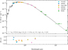 |
Fig. 2 YSES 1 SED fit. The photometric points are colour-coded according to their data source. The black curve shows the best-fit BT-Settl-CIFIST model with a spectral resolution of 100 ( |
![Mathematical equation: $\[\chi_{\nu}^{2}\]$](/articles/aa/full_html/2026/06/aa59005-26/aa59005-26-eq9.png)
Stellar parameters derived for YSES 1 from an SED fit.
3.3 Mass estimate
Using the median bolometric luminosity (log Lp/L⊙) from Table 4 and the age of the system, we obtain an estimate of the mass of the object by fitting an evolutionary model. For the system age we considered two values: the original 16.7 ± 1.4 Myr (Bohn et al. 2020a) and a more recent estimate of 27 ± 3 Myr (Wood et al. 2023). We used the BT-Settl isochrones as our evolutionary model (Allard et al. 2011). Using the nested-sampling fitting procedure of species, we derived posterior distributions for the following parameters: age, mass (M), effective temperature (Teff), radius (Rp) and surface gravity (log g). Table 5 summarises the results and the full posterior distributions can be found in Appendix E. The median estimated mass is either 25.7 MJ or 41.6 MJ, depending on the age of the system. Although evolutionary modelling fits a single luminosity parameter and therefore introduces an ambiguity in the derived effective temperature and radius, the results can be compared with Table 4. The values corresponding to the age of 27 Myr are in better agreement with those derived from the SED fit, indicating that the older age is more consistent with these results.
Parameters derived for YSES 1 b from forward modelling with and without a CPD.
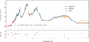 |
Fig. 3 Top: spectral energy distribution (SED) fit of YSES 1 b using MagAO-X, SPHERE, and NACO data using only an atmospheric model. The black line shows the best-fit model ( |
![Mathematical equation: $\[\chi_{\nu}^{2}\]$](/articles/aa/full_html/2026/06/aa59005-26/aa59005-26-eq30.png)
Evolutionary fit for the estimated ages of 16.7 Myr (Bohn et al. 2020a) and 27 Myr (Wood et al. 2023).
4 Discussion
Using only the atmospheric model in Table 4, we compared the retrieved parameters with those in Figure 5 of Bohn et al. (2020a) to test if our SED fit with MagAO-X data is consistent. The effective temperatures are in good agreement (1784 versus 1727 K). We find median log g and radius values of 5.23 dex and 2.45 RJ, which deviate from the values of 3.91 dex and 3.0 RJ reported by Bohn et al. (2020a), although both remain consistent within the uncertainties. However, Bohn et al. (2020a) achieve a better fit, especially at wavelengths longer than 2 μm. This is due to their use of the original BT-Settl model rather than the CIFIST release. We adopted the CIFIST release because it uses updated solar abundances (Caffau et al. 2011).
Regardless of the atmospheric model used, one key issue is that the estimated radius is still considerably larger than that expected for a low-mass companion (Baraffe et al. 2015). The inclusion of a blackbody component by Hoch et al. (2025) to model the CPD still results in a radius of 3 RJ from forward modelling. Using the CPD model in this work, which includes both dust extinction and a blackbody component, reduces the radius to 1.58 RJ, in much better agreement with the expected radius of a substellar companion of this age. The CPD cavity-size estimate Rring corresponding to ![Mathematical equation: $\[56_{-36}^{+178}\]$](/articles/aa/full_html/2026/06/aa59005-26/aa59005-26-eq40.png) RJ is on the same order of magnitude as the values of 40 ± 0.7 RJ and 33 ± 3 RJ reported for GQ Lup b and Delorme 1 (AB) b (Cugno et al. 2024; Mâlin et al. 2025). Nevertheless, the value derived for YSES 1 b from the SED is much less constrained and therefore difficult to compare. The estimated masses of 25.7 MJ or 41.6 MJ are significantly higher than the 14 MJ reported in Bohn et al. (2020a). Using the 13 MJ threshold, although it does not fully capture the separation between brown dwarfs and planets (Schneider 2018), the newly derived mass more strongly supports a brown dwarf interpretation for YSES 1 b.
RJ is on the same order of magnitude as the values of 40 ± 0.7 RJ and 33 ± 3 RJ reported for GQ Lup b and Delorme 1 (AB) b (Cugno et al. 2024; Mâlin et al. 2025). Nevertheless, the value derived for YSES 1 b from the SED is much less constrained and therefore difficult to compare. The estimated masses of 25.7 MJ or 41.6 MJ are significantly higher than the 14 MJ reported in Bohn et al. (2020a). Using the 13 MJ threshold, although it does not fully capture the separation between brown dwarfs and planets (Schneider 2018), the newly derived mass more strongly supports a brown dwarf interpretation for YSES 1 b.
A comparison between the JWST (Hoch et al. 2025) flux and the existing SPHERE and NACO photometry shows a significant difference. This is shown in Figure 5, where we plot the JWST/NIRSpec data and the ground-based photometry. The ground-based and space-based data are consistent up to 1.2 μm. At wavelengths longer than 1.2 μm, JWST shows a significantly lower flux than the ground-based measurements. The difference between the best-fit model and the JWST NIRSpec spectrum in this wavelength range is approximately 15–45%. We re-reduced the SPHERE data to search for an explanation for this discrepancy, but we found the same contrast levels as before. In addition, we compared the contrast in the SPHERE K1 and K2 filters to recently published GRAVITY K-band spectra and found them to be consistent (Kammerer et al. 2025). Variability in YSES 1 b may be considered in this context. Other young planet and brown dwarf companions show variability due to cloud cover. Nevertheless, the reported levels of variability are generally lower, ranging from the percent level to the 26% percent reported by Radigan et al. (2012) (Biller 2017; Sutlieff et al. 2023). Furthermore, the newly derived effective temperature is too high to expect cloud condensation to occur, so the variability would need to arise from a different source. Variability in the dust extinction would lead to the largest discrepancies at short wavelengths, but the JWST data are consistent at wavelengths below 1.2 μm. In addition, the ground-based data were taken at different epochs and show consistent results, which makes a strong variability scenario less favourable. Therefore, future work and observations at different epochs are needed to validate the cause of the discrepancy.
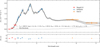 |
Fig. 4 Top: spectral energy distribution (SED) fit of YSES 1 b using MagAO-X, SPHERE, and NACO data using an atmospheric model in combination with a dust extinction model and blackbody radiation to represent the CPD. The black line shows the best-fit ( |
![Mathematical equation: $\[\chi_{\nu}^{2}\]$](/articles/aa/full_html/2026/06/aa59005-26/aa59005-26-eq39.png)
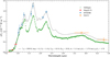 |
Fig. 5 Comparison of ground-based photometry and our best-fit model to the JWST NIRSpec data. |
5 Conclusions
We obtained data on YSES 1 b in the r′, i′ and z′ bands using MagAO-X. We clearly detect YSES 1 b in the i′ and z′ filters, while we derive only an upper limit in the r′ band. The MagAO-X data are consistent with models fitted to the existing SPHERE and NACO photometry. We included a model of the CPD which was recently confirmed using JWST (Hoch et al. 2025). Adding dust extinction and blackbody emission led to an SED that, compared to the initial characterisation of YSES 1 b by Bohn et al. (2020a), is significantly more massive (![Mathematical equation: $\[25.7_{-3.6}^{+4.1}\]$](/articles/aa/full_html/2026/06/aa59005-26/aa59005-26-eq41.png) or
or ![Mathematical equation: $\[41.6_{-3.4}^{+3.6}\]$](/articles/aa/full_html/2026/06/aa59005-26/aa59005-26-eq42.png) MJ versus 14±3 MJ), warmer (
MJ versus 14±3 MJ), warmer (![Mathematical equation: $\[2854_{-94}^{+110}\]$](/articles/aa/full_html/2026/06/aa59005-26/aa59005-26-eq43.png) K versus
K versus ![Mathematical equation: $\[1727_{-127}^{+172}\]$](/articles/aa/full_html/2026/06/aa59005-26/aa59005-26-eq44.png) K), and smaller (
K), and smaller (![Mathematical equation: $\[1.58_{-0.07}^{+0.06}\]$](/articles/aa/full_html/2026/06/aa59005-26/aa59005-26-eq45.png) RJ versus
RJ versus ![Mathematical equation: $\[3.0_{-0.7}^{+0.2}\]$](/articles/aa/full_html/2026/06/aa59005-26/aa59005-26-eq46.png) RJ). This suggests that YSES 1 b is more likely to lie in the brown dwarf regime rather than the planet regime. It also resolves the previously identified large-radius anomaly, as the newly determined radius is consistent with those of other young planets and brown dwarfs.
RJ). This suggests that YSES 1 b is more likely to lie in the brown dwarf regime rather than the planet regime. It also resolves the previously identified large-radius anomaly, as the newly determined radius is consistent with those of other young planets and brown dwarfs.
Acknowledgements
This work is financially supported by the Netherlands Organisation for Scientific Research NWO (Vidi 213.149). We thank Kielan Hoch for sharing the JWST/NIRSpec spectrum. We are very grateful for support from the NSF MRI Award #1625441. The Phase II upgrade program is made possible by the generous support of the Heising-Simons Foundation. The development of CACAO is supported by NSF Award #2410616.
References
- Allard, F. 2013, Proc. Int. Astron. Union, 8, 271 [Google Scholar]
- Allard, F., Homeier, D., & Freytag, B. 2011, in ASP Conference Series, 448 (Astronomical Society of the Pacific) [Google Scholar]
- Amara, A., & Quanz, S. P. 2012, MNRAS, 427, 948 [Google Scholar]
- Bailer-Jones, C. A. L., Rybizki, J., Fouesneau, M., Demleitner, M., & Andrae, R. 2021, AJ, 161, 147 [Google Scholar]
- Bailey, V., Hinz, P. M., Currie, T., et al. 2013, ApJ, 767, 31 [Google Scholar]
- Baraffe, I., Homeier, D., Allard, F., & Chabrier, G. 2015, A&A, 577, A42 [NASA ADS] [CrossRef] [EDP Sciences] [Google Scholar]
- Bayo, A., Rodrigo, C., Barrado Y Navascués, D., et al. 2008, A&A, 492, 277 [NASA ADS] [CrossRef] [EDP Sciences] [Google Scholar]
- Benisty, M., Bae, J., Facchini, S., et al. 2021, ApJ, 916, L2 [NASA ADS] [CrossRef] [Google Scholar]
- Betti, S. K., Follette, K. B., Ward-Duong, K., et al. 2022, ApJ, 935, L18 [NASA ADS] [CrossRef] [Google Scholar]
- Beuzit, J.-L., Vigan, A., Mouillet, D., et al. 2019, A&A, 631, A155 [NASA ADS] [CrossRef] [EDP Sciences] [Google Scholar]
- Biller, B. 2017, AR, 13, 1 [Google Scholar]
- Bohn, A. J., Kenworthy, M. A., Ginski, C., et al. 2020a, MNRAS, 492, 431 [Google Scholar]
- Bohn, A. J., Kenworthy, M. A., Ginski, C., et al. 2020b, ApJ, 898, L16 [Google Scholar]
- Bohn, A. J., Ginski, C., Kenworthy, M. A., et al. 2021, A&A, 648, A73 [NASA ADS] [CrossRef] [EDP Sciences] [Google Scholar]
- Bowler, B. P., Liu, M. C., Kraus, A. L., Mann, A. W., & Ireland, M. J. 2011, ApJ, 743, 148 [Google Scholar]
- Bowler, B. P., Andrews, S. M., Kraus, A. L., et al. 2015, ApJ, 805, L17 [Google Scholar]
- Buchner, J., Georgakakis, A., Nandra, K., et al. 2014, A&A, 564, A125 [NASA ADS] [CrossRef] [EDP Sciences] [Google Scholar]
- Caffau, E., Ludwig, H.-G., Steffen, M., Freytag, B., & Bonifacio, P. 2011, Sol. Phys., 268, 255 [Google Scholar]
- Close, L. M., Males, J. R., Durney, O., et al. 2018, in Adaptive Optics Systems VI, 10703 (SPIE), 107034Y [Google Scholar]
- Cugno, G., & Grant, S. L. 2025, ApJ, 991, L46 [Google Scholar]
- Cugno, G., Patapis, P., Banzatti, A., et al. 2024, ApJ, 966, L21 [NASA ADS] [CrossRef] [Google Scholar]
- Currie, T., Biller, B., Lagrange, A.-M., et al. 2023, in ASP Conference Series, Vol. 534 (Astronomical Society of the Pacific), 799 [Google Scholar]
- Cutri, R. M., Skrutskie, M. F., van Dyk, S., et al. 2003, 2MASS All Sky Catalog of point sources (Infrared Science Archive) [Google Scholar]
- Cutri, R. M., Wright, E. L., Conrow, T., et al. 2012, Explanatory Supplement to the WISE All-Sky Data Release Products [Google Scholar]
- Demars, D., Bonnefoy, M., Dougados, C., et al. 2025, A&A, 706, A57 [Google Scholar]
- Epchtein, N., Deul, E., Derriere, S., et al. 1999, A&A, 349, 236 [NASA ADS] [Google Scholar]
- Foreman-Mackey, D. 2016, JOSS, 1, 24 [NASA ADS] [CrossRef] [Google Scholar]
- Foreman-Mackey, D., Hogg, D. W., Lang, D., & Goodman, J. 2013, PASP, 125, 306 [Google Scholar]
- Gaia Collaboration (Vallenari, A., et al.) 2023, A&A, 674, A1 [NASA ADS] [CrossRef] [EDP Sciences] [Google Scholar]
- Gordon, K. D., Clayton, G. C., Decleir, M., et al. 2023, ApJ, 950, 86 [CrossRef] [Google Scholar]
- Haffert, S. Y., Bohn, A. J., De Boer, J., et al. 2019, Nat. Astron., 3, 749 [CrossRef] [Google Scholar]
- Henden, A. A., Templeton, M., Terrell, D., et al. 2016, VizieR Online Data Catalog: II/336 [NASA ADS] [Google Scholar]
- Hoch, K. K. W., Rowland, M., Petrus, S., et al. 2025, Nature, 643, 938 [Google Scholar]
- Høg, E., Fabricius, C., Makarov, V. V., et al. 2000, A&A, 363, 385 [Google Scholar]
- Holstein, R. G. v., Stolker, T., Jensen-Clem, R., et al. 2021, A&A, 647, A21 [NASA ADS] [CrossRef] [EDP Sciences] [Google Scholar]
- Julo, R., Bonnefoy, M., Chatelain, F., et al. 2025, A&A, 703, A205 [NASA ADS] [CrossRef] [EDP Sciences] [Google Scholar]
- Kammerer, J., Winterhalder, T. O., Lacour, S., et al. 2025, A&A, 704, A318 [NASA ADS] [CrossRef] [EDP Sciences] [Google Scholar]
- Kennedy, G. M., & Wyatt, M. C. 2014, MNRAS, 444, 3164 [NASA ADS] [CrossRef] [Google Scholar]
- Lenzen, R., Hartung, M., Brandner, W., et al. 2003, Proc. SPIE 4841, 944 [Google Scholar]
- Long, J. D., Pearce, L., Haffert, S. Y., et al. 2025, AJ, 169, 36 [Google Scholar]
- MacKay, D. J. C. 2003, Information Theory, Inference, and Learning Algorithms (Cambridge University Press) [Google Scholar]
- Males, J. R., Close, L. M., Haffert, S. Y., et al. 2024, in Adaptive Optics Systems IX, 13097 (SPIE), 1309709 [Google Scholar]
- Marois, C., Lafreniere, D., Doyon, R., Macintosh, B., & Nadeau, D. 2006, ApJ, 641, 556 [NASA ADS] [CrossRef] [Google Scholar]
- Mâlin, M., Ward-Duong, K., Grant, S. L., et al. 2025, A&A, 704, A181 [NASA ADS] [CrossRef] [EDP Sciences] [Google Scholar]
- Pecaut, M. J., & Mamajek, E. E. 2016, MNRAS, 461, 794 [Google Scholar]
- Radigan, J., Jayawardhana, R., Lafrenière, D., et al. 2012, ApJ, 750, 105 [NASA ADS] [CrossRef] [Google Scholar]
- Roberts, J., Thompson, W., Wang, J. J., et al. 2025, AJ, 170, 273 [Google Scholar]
- Rousset, G., Lacombe, F., Puget, P., et al. 2003, Proc. SPIE, 4839 [Google Scholar]
- Schneider, J. 2018, in Handbook of Exoplanets, eds. H. J. Deeg, & J. A. Belmonte (Cham: Springer International Publishing), 611 [Google Scholar]
- Stolker, T., Bonse, M. J., Quanz, S. P., et al. 2019, A&A, 621, A59 [NASA ADS] [CrossRef] [EDP Sciences] [Google Scholar]
- Stolker, T., Quanz, S. P., Todorov, K. O., et al. 2020, A&A, 635, A182 [EDP Sciences] [Google Scholar]
- Stolker, T., Haffert, S. Y., Kesseli, A. Y., et al. 2021, AJ, 162, 286 [NASA ADS] [CrossRef] [Google Scholar]
- Sutlieff, B. J., Birkby, J. L., Stone, J. M., et al. 2023, MNRAS, 520, 4235 [NASA ADS] [CrossRef] [Google Scholar]
- Wood, M. L., Mann, A. W., Barber, M. G., et al. 2023, AJ, 165, 85 [NASA ADS] [CrossRef] [Google Scholar]
- Zhang, Y., Snellen, I. A. G., Bohn, A. J., et al. 2021, Nature, 595, 370 [NASA ADS] [CrossRef] [Google Scholar]
- Zhang, Y., Picos, D. G., Regt, S. d., et al. 2024, AJ, 168, 246 [NASA ADS] [CrossRef] [Google Scholar]
- Zhou, Y., Herczeg, G. J., Kraus, A. L., Metchev, S., & Cruz, K. L. 2014, ApJ, 783, L17 [Google Scholar]
Appendix A Posterior distributions for separation, position angle, and contrast for YSES 1 b
The posterior distributions of the separation, position angle, and contrast of YSES 1 b in the MagAO-X i′-filter and z′-filter as estimated by the MCMC analysis.
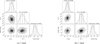 |
Fig. A.1 The posterior distributions for fitting the contrast and astrometry of YSES 1 b in the i′-filter and z′-filter using the negative artificial planet injection of PynPoint and the emcee sampler (Foreman-Mackey et al. 2013). The plot was made using corner.py (Foreman-Mackey 2016). |
Appendix B Estimated offsets from systematics analysis
The offset in separation, position angle, and contrast which is estimated by finding the difference between the injected and retrieved values at different locations.
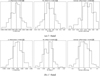 |
Fig. B.1 The estimated distributions for the separation, position angle, and contrast offsets for the i′-filter and z′-filter. The difference between the injected and retrieved values was evaluated at 250 different position angle locations at the separation of YSES 1 b. |
Appendix C Posterior distributions of the YSES 1 SED fits
Posterior distributions of the stellar SED fit for YSES 1.
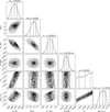 |
Fig. C.1 The posterior distributions for the stellar SED fit using the BT-Settl-CIFIST model. The nested sampling was performed using species which utilises the MultiNest package (Buchner et al. 2014). The plot was made using corner.py (Foreman-Mackey 2016). |
Appendix D Posterior distributions of the YSES 1 b SED fits
Posterior distributions of the SED fits for the atmospheric model and the atmospheric + CPD model.
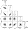 |
Fig. D.1 The posterior distributions for fitting the BT-Settl-CIFIST atmospheric model to the photometric data from MagAO-X, SPHERE and NACO. The nested sampling was performed using species which utilises the MultiNest package (Buchner et al. 2014). The plot was made using corner.py (Foreman-Mackey 2016). |
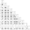 |
Fig. D.2 The posterior distributions for fitting the BT-Settl-CIFIST atmospheric model combined with dust extinction and a disc blackbody component to the photometric data from MagAO-X, SPHERE and NACO. The nested sampling was performed using species which utilises the MultiNest package (Buchner et al. 2014). The plot was made using corner.py (Foreman-Mackey 2016). |
Appendix E Posterior distributions of evolutionary model fits
Posterior distributions of the evolutionary model fit for YSES 1 b using the estimated age of 16.7 or 27 Myr.
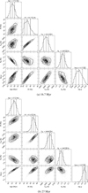 |
Fig. E.1 The posterior distributions for fitting the BT-Settl evolutionary model to the luminosity found in Fig. D.2 and assuming a system age of 16.7 Myr or 27 Myr. The nested sampling was performed using species which utilises the MultiNest package (Buchner et al. 2014). The plot was made using corner.py (Foreman-Mackey 2016). |
All Tables
Evolutionary fit for the estimated ages of 16.7 Myr (Bohn et al. 2020a) and 27 Myr (Wood et al. 2023).
All Figures
|
Fig. 1 Reduced MagAO-X images of the YSES 1 system in the r′, i′ and z′ filters after PCA-based PSF subtraction and Gaussian filtering. The point sources on the top are confirmed background stars (Bohn et al. 2020a). YSES 1 b is recovered in the i′ and z′ bands with an S/N of 13.0 and 11.2, respectively. |
| In the text | |
|
Fig. 2 YSES 1 SED fit. The photometric points are colour-coded according to their data source. The black curve shows the best-fit BT-Settl-CIFIST model with a spectral resolution of 100 ( |
| In the text | |
|
Fig. 3 Top: spectral energy distribution (SED) fit of YSES 1 b using MagAO-X, SPHERE, and NACO data using only an atmospheric model. The black line shows the best-fit model ( |
| In the text | |
|
Fig. 4 Top: spectral energy distribution (SED) fit of YSES 1 b using MagAO-X, SPHERE, and NACO data using an atmospheric model in combination with a dust extinction model and blackbody radiation to represent the CPD. The black line shows the best-fit ( |
| In the text | |
|
Fig. 5 Comparison of ground-based photometry and our best-fit model to the JWST NIRSpec data. |
| In the text | |
|
Fig. A.1 The posterior distributions for fitting the contrast and astrometry of YSES 1 b in the i′-filter and z′-filter using the negative artificial planet injection of PynPoint and the emcee sampler (Foreman-Mackey et al. 2013). The plot was made using corner.py (Foreman-Mackey 2016). |
| In the text | |
|
Fig. B.1 The estimated distributions for the separation, position angle, and contrast offsets for the i′-filter and z′-filter. The difference between the injected and retrieved values was evaluated at 250 different position angle locations at the separation of YSES 1 b. |
| In the text | |
|
Fig. C.1 The posterior distributions for the stellar SED fit using the BT-Settl-CIFIST model. The nested sampling was performed using species which utilises the MultiNest package (Buchner et al. 2014). The plot was made using corner.py (Foreman-Mackey 2016). |
| In the text | |
|
Fig. D.1 The posterior distributions for fitting the BT-Settl-CIFIST atmospheric model to the photometric data from MagAO-X, SPHERE and NACO. The nested sampling was performed using species which utilises the MultiNest package (Buchner et al. 2014). The plot was made using corner.py (Foreman-Mackey 2016). |
| In the text | |
|
Fig. D.2 The posterior distributions for fitting the BT-Settl-CIFIST atmospheric model combined with dust extinction and a disc blackbody component to the photometric data from MagAO-X, SPHERE and NACO. The nested sampling was performed using species which utilises the MultiNest package (Buchner et al. 2014). The plot was made using corner.py (Foreman-Mackey 2016). |
| In the text | |
|
Fig. E.1 The posterior distributions for fitting the BT-Settl evolutionary model to the luminosity found in Fig. D.2 and assuming a system age of 16.7 Myr or 27 Myr. The nested sampling was performed using species which utilises the MultiNest package (Buchner et al. 2014). The plot was made using corner.py (Foreman-Mackey 2016). |
| In the text | |
Current usage metrics show cumulative count of Article Views (full-text article views including HTML views, PDF and ePub downloads, according to the available data) and Abstracts Views on Vision4Press platform.
Data correspond to usage on the plateform after 2015. The current usage metrics is available 48-96 hours after online publication and is updated daily on week days.
Initial download of the metrics may take a while.