| Issue |
A&A
Volume 708, April 2026
|
|
|---|---|---|
| Article Number | A325 | |
| Number of page(s) | 15 | |
| Section | Extragalactic astronomy | |
| DOI | https://doi.org/10.1051/0004-6361/202558816 | |
| Published online | 21 April 2026 | |
A broker-integrated algorithm for electromagnetic counterpart searches to gravitational-wave events in O4a and O4b runs
1
Departamento de Astronomia (DAS), Universidad de Chile, Camino el Observatorio 1515, Las Condes, Santiago, Chile
2
Data and Artificial Intelligence Initiative (IDIA), Faculty of Physical and Mathematical Sciences, Universidad de Chile, Santiago, Chile
3
Centro de Excelencia en Astrofisica y Technologia Afines, Av. Vicuña Mackenna 4860, San Joaquín, Santiago, Chile
4
Millennium Institute of Astrophysics, Nuncio Monseñor Sotero Sanz 100, Of. 104, Providencia, Santiago, Chile
5
Center for Mathematical Modeling, Universidad de Chile, Beauchef 851, Santiago 8370456, Chile
6
Physik-Institut, Universität Zürich, Winterthurerstrasse 190, CH-8057 Zürich, Switzerland
7
Instituto de Astrofísica, Facultad de Física, Pontificia Universidad Católica de Chile, Campus San Joaquín, Av. Vicuña Mackenna 4860 Macul Santiago, 7820436, Chile
8
Centro de Astronomia, Universidad de Antofogasta, 02800 Antofagasta, Chile
9
UKIRT Observatory, Institute for Astronomy, 640 N. A’ohoku Place, University Park, Hilo, Hawai’i, 96720, USA
10
Instituto de Estudios Astrofísicos, Facultad de Ingeniería y Ciencias, Universidad Diego Portales, Av. Ejército Libertador 441 Santiago, Chile
11
Centro Interdisciplinario de Data Science, Facultad de Ingeniería y Ciencias, Universidad Diego Portales, Av. Ejército Libertador 441 Santiago, Chile
12
Astronomy Department, Universidad de Concepción, Casilla 160-C, 4030000 Concepción, Chile
13
Millennium Nucleus on Transversal Research and Technology to Explore Supermassive Black Holes (TITANs), Concepción, Chile
★ Corresponding author: This email address is being protected from spambots. You need JavaScript enabled to view it.
Received:
29
December
2025
Accepted:
9
March
2026
Abstract
Context. We present an automated framework for a search for optical counterparts of LIGO–Virgo–KAGRA (LVK) gravitational-wave (GW) superevents using public Zwicky Transient Facility (ZTF) alerts processed through the Automatic Learning for the Rapid Classification of Events (ALeRCE) broker.
Aims. The goal is to filter and identify optical transients that might be associated with binary black hole (BBH) mergers during the LVK O4a and O4b observing runs.
Methods. Using the infrastructure called ALeRCE, we spatially queried ZTF alerts within GW localization regions and applied machine-learning classifiers, host-galaxy cross-matching, and temporal cuts within 200 days post merger to isolate plausible candidates.
Results. Our search yielded one candidate in O4a and four in O4b, several of which are consistent with the supernova (SN) – tidal disruption event (TDE) regime. This work demonstrates that public-alert brokers can set a baseline for performing systematic searches for electromagnetic counterparts of GW superevents in current and future observing runs.
Conclusions. Our algorithm provides a way to search for the BBH counterparts for all significant LVK GW superevents using survey telescope alerts. The search and the accompanying analysis demonstrate the significance of the counterpart candidates. One candidate, consistent with a Bowen fluorescence flare in an active galactic nucleus, is ultimately disfavored as a counterpart.
Key words: methods: data analysis / surveys / stars: black holes / quasars: supermassive black holes
© The Authors 2026
 Open Access article, published by EDP Sciences, under the terms of the Creative Commons Attribution License (https://creativecommons.org/licenses/by/4.0), which permits unrestricted use, distribution, and reproduction in any medium, provided the original work is properly cited.
This article is published in open access under the Subscribe to Open model. This email address is being protected from spambots. You need JavaScript enabled to view it. to support open access publication.
1. Introduction
Since the first observation of a gravitational wave (GW) by the detectors of Laser Interferometer Gravitational-Wave Observatory, Virgo Interferometer, and Kamioka Gravitational Wave Detector (here after LVK) (Abbott et al. 2016), a total of 391 gravitational wave candidates have been detected as of the end of the fourth observing run (O4). Of these events, binary black hole (BBH) mergers are the dominant class. They account for more than 98% of all the detections. Broadly, the formation channels of the mergers can be classified into isolated and dynamic (Mapelli 2020). The BBH event GW150921 has been proposed to be an example of the dynamic formation channel, with a possible association with the disk environment of an active galactic nucleus ((AGN); Graham et al. 2020), and a light curve consistent with a post-merger disk-flaring event (object ZTF19abanrhr).
Several studies have estimated BBH merger rates in AGN accretion disks (Ford & McKernan 2022; Gröbner et al. 2020; McKernan et al. 2018). Recently, Ford & McKernan (2022) have estimated the rate of R ∼ 24 Gpc−3 yr−1, which they calculated analytically based on the binary lifetime, binary fraction, active lifetime of galactic nuclei, and their AGN fraction. This rate broadly falls in the range of rates predicted by the LVK collaboration R ∼ (17.9 − 44) Gpc−3 yr−1 for z = 0.2 (Abbott et al. 2023), scaling with redshift as (1 + z)k, with  for z ≤ 1. In the AGN environment, high escape velocities allow retention of BBH merger products (Samsing et al. 2022) and the dissipative AGN gas environment allows BHs to pair up again and grow through hierarchical mergers (Tagawa et al. 2020, 2021; Gilbaum et al. 2025). The interaction of the merged BBH with the AGN accretion disk can produce an electromagnetic (EM) counterpart. The merged product receives a recoil velocity, which is a function of the binary mass asymmetry and spin orientation (Baker et al. 2008). The remnant might interact with the gas via Bondi-Hoyle-Lyttleton (BHL) accretion. This can lead to the production of detectable luminosity at super-Eddington rates (Graham et al. 2020), along with jetted outflows that allow radiation to escape and emerge (Wang et al. 2021). The counterpart can emerge weeks to months after the event occurs, modulated by the diffusion timescale of the AGN disk. Modern time-domain surveys scanning the sky with cadences of weeks to months might be helpful in identifying and monitoring these transients.
It is challenging to distinguish these counterparts from the innate AGN variability and different types of nuclear transient events such as supernoave (SN), tidal disruption events (TDEs), and microlensing close to the supermassive black hole (SMBH). Moreover, alternative mechanisms have been developed that might result in the production of an EM counterpart along with the GW (McKernan et al. 2012; Bartos et al. 2017; Kimura et al. 2021; Perna et al. 2021; Wang et al. 2021; Rodríguez-Ramírez et al. 2025; Tagawa et al. 2023).
Many collaborations such as GW-MMADS (Kunnumkai et al. 2024), GRANDMA (Agayeva et al. 2022), and DESGW (Herner et al. 2020) are actively searching for the counterparts of gravitational sources. Web-based target and observation managers from centralized portals such as SAGUARO (Hosseinzadeh et al. 2024) and SkyPortal (Coughlin et al. 2023) have been built to reduce the need for human intervention and improve coordination in the search for the counterparts. However, this search is usually only conducted when the localization area of GW event is quite small (< 100 deg2).
In the era of big data astronomy, so-called alert brokers ingest, annotate, filter, and classify astronomical alerts from survey telescopes such as the Zwicky transient Facility (ZTF, Bellm et al. 2018), the Asteroid Terrestrial-impact Last Alert System (ATLAS, Tonry et al. 2018), the La Silla Schmidt Southern Survey (LS4, Miller et al. 2025), and the survey Legacy Survey of Space and Time (LSST, Ivezić et al. 2019) for the astronomy community. Of the existing alert brokers, ANTARES (Matheson et al. 2021) and FINK (Möller et al. 2021) also cross match alerts with LVK sky maps.
We took advantage of the public alerts from ZTF and classification algorithms of the broker called ALeRCE (Förster et al. 2021) to search for the counterparts of BBH mergers in AGN in an untargeted fashion, that is, we considered majority of the LVK superevents and their cross matches. We introduce an algorithm that uses the ALeRCE services to search for the optical counterparts of GW sources during the O4 run. Because the data volumes generated by ZTF in the form of alerts is very large, we built an automated pipeline that on receiving LVK alerts (effectively, a sky map), filters only those ZTF events whose localization and redshift (inferred from the LVK alert) are consistent with that of AGNs with a detectable activity within 200 days post merger.
This paper is organized as follows. In Section 2 we introduce the data and the ALeRCE broker. In Section 3 we describe the algorithm we designed to filter the possible counterparts from the alerts. In Section 4 we explain the results of applying the algorithm to the LVK O4a and O4b runs, including the most interesting candidates, and in Section 5 we analyze the results by comparing the expected number and properties of associated flares with our previous findings. Finally, our discussions and conclusions are summarized in Sections 6 and 7.
2. Data
2.1. ZTF
The ZTF (Bellm et al. 2018) has been surveying the northern sky every ∼3 days in the g, r, and i optical filters since 2018 and offers different services, such as (1) a public-alert system for real-time domain science, (2) data releases (DRs) every two months, including photometric measurements on the science images, and (3) a forced-photometry service on demand per source, including the photometry measurements on the reference-subtracted science images.
For the alert to be generated, a source has to show a variation at least five times above the background noise of the difference image (5σ).
We retrieved data from the ZTF forced-photometry Service (Masci et al. 2019, 2023). The measurements from this service are based on reference-subtracted images that isolate the variable nuclear component and reduce contamination from host-galaxy emission compared to public DRs. The light curves were constructed by removing measurements with bad-quality flags, requiring a seeing < 5″ and positive flux uncertainties. Relaxed cuts were applied to preserve faint nuclear variability that might be associated with GW events. No color correction was applied. The difference point spread function magnitudes were converted into apparent magnitudes following Förster et al. (2021).
2.2. ALeRCE annotations
ALeRCE is a Chilean-led broker that processes the alert stream from ZTF. It was selected as a community broker for the Vera C. Rubin Observatory and its Legacy Survey of Space and Time (LSST) and aims to include other large etendue survey telescopes.
ALeRCE1 uses a pipeline that includes real-time ingestion, aggregation, cross-matching, machine-learning (ML) classification and visualization of the ZTF alert stream. We used two classifiers: a stamp-based classifier (Carrasco-Davis et al. 2021) that uses image stamps as input and is designed for rapid classification, and a light-curve-based classifier (Sánchez-Sáez et al. 2021) that uses the multiband flux evolution to achieve a more refined classification.
All alerts associated with new objects undergo the stamp-based classification, which provides a quick classification into a five-class taxonomy (SN, AGN, variable star, asteroid, and bogus). The stamp classifier consists of a rotationally invariant convolutional neural network that uses information from the image stamps and the alert metadata.
2.3. GW sky maps
The GW alerts are distributed in JSON and AVRO formats, which contain key metadata such as the estimated luminosity distance, probabilities among different source classes (e.g., binary black hole, binary neutron star, neutron star black hole, or terrestrial), and significance of the detection. All publicly released alerts are archived in the Gravitational-Wave Candidate Event Database (GraceDB)2. For this work, we retrieved the alerts and associated data products after public release from GraceDB and did not process them in real time. Each alert includes an URL to the corresponding localization sky map (typically, a .fits.gz file), which we used to construct probability maps and perform spatial queries for potential electromagnetic counterparts, as described in Section 3. The 3D localization sky maps are subject to revision when the final O4 catalog is released, and modest changes in the sky-localization volumes or distance posteriors might affect some of the derived association probabilities.
3. Method
3.1. Retrieving GW sky maps
The first step in the search for the optical counterparts of LVK superevents is to obtain their projected spatial probability distribution, which is referred to as sky maps. LVK distribute these sky maps in standard HEALPix (Górski et al. 2005) representation in flat and multiresolution formats. We used the multiresolution sky maps for the counterpart search, assuming that the LVK superevents lie within the 90% integrated probability contours. In general, these sky maps can be obtained from the following sources:
-
The public General Coordinates Network (GCN) alert stream.
-
The Gravitational-Wave candidates event database (GraceDB) web interface3.
-
The gracedb-sdk client4.
The sky maps in this study were built following the instructions in the emfollow website, a LVK public alerts user guide5. An example sky map is depicted in Figure 1.
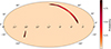 |
Fig. 1. Sky map from LVK of the GW event S240902bq. The color scale represents the probability contours. |
3.2. Performing spatial queries within sky maps
When the sky maps became available, we compared them with ZTF optical-based alerts. We used the ALeRCE broker to access the ZTF alert data.
The time and location of every ZTF alert required is available in ALeRCE PostgreSQL database. The spatial query is performed using the Quad Tree Cube (Q3C, Koposov & Bartunov 2006) PostgreSQL extension. In Q3C, spatial indexing is achieved by projecting the sides of an imaginary cube onto the celestial sphere, where each side is divided into multiple quad tree structures for more efficient querying. In this implementation, the query region is defined by the vertices of a polygon, in this case, the 90% probability contour of the LVK sky maps. However, two limitations are associated with using Q3C: (1) query polygons must not exceed 25 degrees in diameter, and (2) the number of vertices that define the polygon must be smaller than 100.
Because of the limitations and the need to efficiently search within large GW localization regions, we began by transforming the sky-map pixels into a cloud of points. Then, we partitioned the points into multiple spatial clusters using the K-means algorithm. Each cluster consisted of a finite set of HEALPix pixels, each containing spatial and probability information. To enable spatial querying, we converted the pixels within each cluster into bounding polygons using the alphashape library. In contrast to convex hulls, these polygons need to adopt a concave hull geometry because they follow the contours of the sky map more accurately. The degree of concavity is controlled by the α parameter. We found that an alpha value of 0.2 achieves an effective balance between contour fidelity and overfitting. These resulting polygons were then used as spatial regions for querying transient candidates, as illustrated in Figure 2.
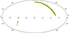 |
Fig. 2. Sky map converted into bounded polygons (green boundaries) filled with ZTF public alerts in yellow. |
The optical counterparts may be long-lived because the diffusion timescales of the SMBH accretion disk is long as BHL accretion takes place. Following (Graham et al. 2023), we defined a maximum search timescale of 200 days post merger to be sensitive enough to kick velocities ≥1 km s−1.
3.3. Refining candidates
After obtaining the database with all the ZTF public alerts (hereafter alerts) within the LVK sky map, we built an algorithm to narrow down the search for the counterparts as described below.
-
A typical spatial query of the alerts in a GW sky map contains ∼106 objects. As an initial filtering step, we selected the alerts in proximity to known AGNs using the MILLIQUAS catalog (hereafter MQUAS, Flesch 2023), a compilation of approximately one million quasars with associated redshifts and other properties. Because of the resolution of ZTF, we retained only events located within 3″ of MQUAS AGNs. This catalog was preferred because it includes redshift information, which is crucial for a distance-based filtering. However, it is important to note that MQUAS predominantly contains sources from the northern hemisphere, a bias stemming from the sky coverage of contributing AGN surveys. Moreover, the sample is contaminated by other sources, which necessitates the use of additional filtering based on ALeRCE features.
-
As a secondary filtering step to exclude likely bogus detections, variable stars, and asteroids, we applied the ALeRCE classifiers (Carrasco-Davis et al. 2021; Sánchez-Sáez et al. 2021). The stamp classifier uses the first image cutouts associated with each alert; specifically, the science, reference, and difference images along with Pan-STARRS metadata, to assign probabilistic classifications. These include SN, AGN, variable star, asteroid, and bogus categories. We retained only candidates for which the combined probability of the SN and AGN classes was greater than or equal to 0.5.
-
We also employed the light-curve classifier, which uses variability features derived from ZTF photometry and color information from the ZTF and ALLWISE (Cutri et al. II/328.). This classifier implements a balanced random forest model trained on sources with at least ndet ≥ 6 detections in either the g or r band. Candidates were retained only when the total probability assigned to the SN or AGN subclasses was greater than or equal to 0.5.
-
An additional filter was applied to exclude star-like sources, incorporating data from the Pan-STARRS (PS1, Chambers et al. 2016) survey. This step keeps candidates with a ZTF real/bogus score ≥0.5 and a star-galaxy score (sgscore) ≤0.5. The sgscore varies between 0 and 1 for galaxies and stars, respectively. This ensured that only real events of extragalactic origin were considered.
-
The fourth cut was based on the location of the event with respect to the Galactic and Solar System planes. First, we kept alerts that occurred in regions with a low Galactic attenuation (Aν < 1). For events in proximity to the Solar System plane (< 20 deg), we required multiple detections (ndet > 1).
-
The fifth and final cut was based on the reported luminosity distance from the LVK events. Only candidates whose MQUAS-reported distance is within 2σ of the LVK luminosity distance mean were retained.
The source code details are provided in the Data availability section.
3.4. Effectiveness of the stamp classifier
As discussed earlier, the impurity of the MQUAS catalog necessitates the use of ALeRCE classifiers. To evaluate the impact of the stamp classifier filter within our algorithm, we categorized the alerts spatially matched to MQUAS AGNs (within 1.4″) using the stamp classifier for the LVK data. This spatial cross match yielded approximately ∼15 059 and ∼10 790 events for O4a and O4b, respectively. Upon applying the ALeRCE stamp classifier, ∼12 544 and ∼8495 of these events were classified as AGNs, with other classes occurring in smaller numbers, as shown in Figure 3. Even though the majority of spatially matched events are already classified as AGNs, this filter provided a cleaner version of the catalog.
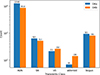 |
Fig. 3. Distribution of classes by stamp classifier for the events originating with 1.4″ of the MQUAS AGN catalog for the O4a and O4b runs. |
3.5. Predicting the chirp mass
For GW superevents that are released to the public during an ongoing LVK observing run, information about the masses involved in the merger is not immediately publicly available6. However, for a time-critical counterpart follow-up of GW events, a rough estimate of the chirp mass of the system can be estimated using the publicly available localization sky map and ML techniques. This is possible because the chirp mass scales directly with the amplitude and luminosity distance of the gravitational wave signal. The luminosity distance is given in the sky map, and information on the signal-to-noise ratio (S/N), and amplitude by proxy, is encoded in the size of the uncertainty region in luminosity distance and sky area.
We used an ordinal class probability density function (OCP) algorithm, that was originally developed to approximate photometric redshift, but we adapted it for mass approximation (Rau et al. 2015). We defined classes using linearly equally divided bins on the chirp mass range [0, 75] M⊙, covering the compact object mergers observed by LVK (The LIGO Scientific Collaboration et al. 2025) and predicted by population synthesis models (Belczynski et al. 2020; Gerosa & Fishbach 2021). We trained the random forest classifier, provided by the SKLEARN package (Pedregosa et al. 2011) to estimate the probability that a given event had a chirp mass inside each mass bin. We then used a Gaussian kernel density estimation (KDE) to estimate a continuous probability density function, and from this KDE, we obtained a final estimated median value of the chirp mass with upper and lower bounds. The input vector for each event is given by the HEALPix pixel index, probability, luminosity distance, and luminosity distance error for each of the 20 highest probability pixels in the event sky map, downsampled to HEALPix NSIDE = 8. We found that these values were sufficient to encode the direction, amplitude, and distance for the chirp mass estimation.
For training data, we simulated 368 000 events using BAYESTAR (Singer & Price 2016). We used a logarithmic component mass distribution in the range [1.2, 75] M⊙ and a distance distribution that was uniform in volume out to 6000 Mpc. We assumed aligned spins from the range [0, 0.05] and a network S/N detection threshold of 8. We used the default noise curves for the LIGO/Virgo detectors in O4 implemented in BAYESTAR. Out of our simulated events, 13 757 events surpassed the network detection threshold and were used for training. We found that we generally recovered true chirp mass values with 50% error bounds and a slight bias at the mass range boundaries (see Figure A.1).
4. Results
During the O4 observing run of the LVK Collaboration, significant improvements were implemented in the low-latency detection pipelines, particularly in background estimation and event ranking. This resulted in slightly lower thresholds of the false-alarm rate. Combined with enhanced detector sensitivities relative to previous runs, these updates resulted in a substantial increase in the number of detected low-significance candidates, including several single-detector triggers with a large sky-map area (The LIGO Scientific Collaboration et al. 2025; Petrov et al. 2022; Soni et al. 2025). Single-detector superevents generally have poor sky localization and low astrophysical probability, making them less suitable for electromagnetic follow-up. Therefore, we only considered multidetector detections, which provide a higher network S/N and more reliable localization posteriors for a cross match with optical transient surveys and AGN catalogs.
The distribution of areas and the median area for the O4a and O4b runs is shown in Figure 4. The involvement of an additional detector during the O4b run demonstrated the decrease in the median area from the O4a to O4b run.
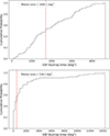 |
Fig. 4. Cumulative distribution function of the sky-map areas for O4a (top) and O4b (bottom) with median area values (vertical red lines). |
Figures 5 and 6 represent the number of events through different filters/cuts applied on alerts in the O4a and O4b runs. The number of alerts in the proximity of MQUAS AGNs differs by a factor of 1000 from that of the total ZTF-LVK cross-matched events.
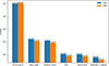 |
Fig. 5. Total number of events for both runs, including all filters. |
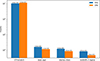 |
Fig. 6. Total number of events for both runs, excluding PS1 and location-based filter. |
4.1. ZTF candidates
The implementation of the algorithm on multidetector GW superevents yielded 602 and 380 candidates for the O4a and O4b observing runs, respectively. After visual inspection and excluding alerts already classified as SN or TDE on the Transient Name Server (TNS), we identified one interesting candidate, ZTF23abqkwzr, from O4a and four interesting candidates from O4b: ZTF25aagpypz, ZTF25aafwffi, ZTF24absmrlr, and ZTF24abricne.
To investigate whether these transients were nuclear in origin, we employed an improved version of the classifier described in Pavez-Herrera et al. (2025). The original classifier included TDEs as a separate class, while the new version introduces nuclear transients (NTs). This broader category encompasses known optical TDEs and ambiguous nuclear transients (ANTs). This updated classifier is currently under development (Pávez-Herrera et al., in prep.). Its inputs consist of ZTF-alert light curves along with additional metadata from the alerts. This new version also differs from the previous one in that it includes additional features based on multiband light-curve fitting, such as those provided by the rainbow algorithm (Russeil et al. 2024).
The parametric models described in Pavez-Herrera et al. (2025) such as the decay and a ML algorithm optimized for identifying TDEs (FLEET, Gomez et al. 2023), were updated to follow this multiband approach by fitting independently to each band, and the sum of the errors across all bands was then optimized while introducing a regularization term that encourages some parameters to remain similar between bands. Furthermore, the probability outputs are more realistic because they were calibrated using CALIBRATIONCV from SKLEARN.
Thus, the code classified three of the transients as NTs, as represented in Table 1. In the case of ZTF23abqkwzr, the highest classification probability for an AGN with 0.52, the second highest probability is for an NT with 0.33. Despite the transient light curve, the object was classified as a AGN by ePESSTO+ when the flux was rising (Ihanec et al. 2024).
Nuclear transient classifier results.
4.2. GW-EM parameter inference
The GW parameter, specifically, the chirp mass, can be estimated using the algorithm described in Section 3.5. The potential electromagnetic (EM) light curves arising from the motion of the remnant black hole within the accretion disk leading to BHL accretion can be modeled using the framework and equations presented in Graham et al. (2023). These models allowed us to explore the possible EM signatures associated with compact object mergers embedded in the AGN disks.
The only parameter that can be directly deduced from the LVK public alerts is the chirp mass, which was estimated using the chirp mass prediction described above. The application of this method to the cross-matched GW superevents yielded the chirp mass values listed in Table 2.
GW superevents and corresponding chirp masses.
The parameter inference for the light curves shown in Figures 7 and 8 was performed for the events listed above using the equations presented in Graham et al. (2023). The exit timescale, texit, is defined as the total time between the GW merger and flare peak. This timescale characterizes the period required for the recoiling merger remnant to interact with and emerge from the surrounding disk material, producing observable emission. The rise and decay times of each event were obtained by fitting a model with a Gaussian rise and an exponential decay profile. The maximum recoil velocity was then computed from the total radiated energy of the light curve, assuming a radiative efficiency of 0.1, a disk density of 10−10 g cm−3, the SMBH mass, and the observed flare timescale, following the prescription of Graham et al. (2023).
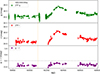 |
Fig. 7. Light curves of the O4a counterpart candidate AT2023zgo/ZTF23abqkwzr in ZTF g and r bands and g-r color for the science images and their forced photometry. The vertical line represents the GW event with which the corresponding ZTF alert might be associated. |
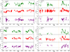 |
Fig. 8. Light curves of O4b counterpart candidates in ZTF g and r bands and g-r color for the science images and their forced photometry. The vertical lines in each plot represent the time of the GW event. |
Using the maximum recoil velocities estimated for each event, and assuming an optical depth τmp ∼ 104.5 (Cabrera et al. 2024) and the inferred exit timescales, we derived disk scale heights of H/Rg ∼ 0.8 − 50, corresponding to physical heights of H ∼ 3 × 10¹³ − 1 × 1014 cm for SMBH masses of 107.1 − 108.4 M⊙. These values represent upper limits on the disk thickness, because they are based on the maximum plausible recoil velocities. The resulting H/Rg ratios are consistent with those expected for the thin to moderately thick regions of AGN accretion disks, as predicted by analytic models (e.g., Sirko & Goodman 2003; Thompson et al. 2005). The derived parameters for each event are summarized in Table 3, while a detailed multiwavelength spectral analysis of the O4a counterpart candidate is presented in Appendix B. The g-band light curves were considered for the parameter inference.
ZTF events and corresponding GW superevents with location, light curve, and AGN properties.
5. Analysis
In this section, we evaluate the likelihood of random associations between AGN flares and LVK GW events. Previously, Graham et al. (2020), who reported the first possible association between a GW event and an AGN flare, and, Graham et al. (2023), who extended this analysis to the full LVK O3 run, have demonstrated the potential for detecting optical counterparts to BBH mergers. In particular, Graham et al. (2023) identified 20 AGN flares in ZTF Data Release 5 (2018–2021) over a period of ∼1000 days after excluding known SNe, TDEs, and microlensing events. Seven of these flares were spatially and temporally coincident with nine GW events from the O3 observing run, which lasted 11 months. Assuming these associations are random coincidences (Veronesi et al. 2024), we adopted this result as a normalization factor.
5.1. Simulating random AGN flares
To evaluate the expected rate of chance associations between AGN flares and GW events, we simulated a population of flaring AGNs. We assumed that non-GW related AGN flares dominate the population of AGN flares. We randomly selected ∼650 flaring AGNs from the MQUAS catalog and assigned each a flare time (MJD) randomly distributed between the start of the O4 subrun and up to 200 days after its end. Using the public ZTF survey pointing history (Figure 9), we assessed for each LVK sky map from the O4 subruns whether a given flare would have been detected within the observed fields. This is within a 200-day time frame post merger and a 2σ distance limit of the respective GW event inferred distance.
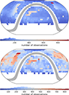 |
Fig. 9. ZTF pointings for public alerts based on the quality assurance product for O4a (top) and O4b (bottom) with npointings ≥ 15, where the color scale represents the observation frequency. |
5.2. Expected number of flares
We started by measuring the number of randomly associated flares as a function of the GW sky-map area. To do this, we measured the number of detected flares among those simulated for different GW sky-map area thresholds. These values were normalized relative to those reported by Graham et al. (2023), so that we recovered about 20 flares in AGNs of MQUAS per 1000 days, independent of the GW events.
The simulated detection statistics were then compared with the observed events (mentioned in the previous section) in terms of the cumulative number of detections as a function of the GW sky-map area threshold (see Figure 10). The comparison revealed an excess in the number of detected events relative to the random expectation, with one excess event identified during the O4a run and four excess events during the O4b run. In O4a, when we considered a GW sky-map area threshold of 2000 deg2, the probability of having one or more random associations was 7.6 ± 2.5% (1σ). In O4b, when we considered a GW sky-map area threshold of 15 000 deg2, the probability of having three or more random associations was 0.6 ± 0.3% (1σ). This suggests that we can marginally discard the possibility that the observed events are random associations in O4b superevents.
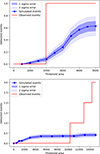 |
Fig. 10. Cumulative distribution function of the simulated (blue) and detected flare events (red) corresponding to ZTF pointings up to 200 days post merger for each GW event as a function of GW sky-map area. The top panel corresponds to O4a, and the bottom panel corresponds to O4b. |
5.2.1. O4b sky-map area distribution
We further statistically tested and analyzed the O4b real and simulated event distributions to strengthen or discard our hypothesis. Instead of only comparing the expected number of events for a given threshold sky-map area, we tested whether the distribution of AGN flare associated sky-map areas resembled those from O4b.
To do this, we introduced a slight modification of the simulation framework: AGN flares were uniquely associated with GW events through a likelihood-based matching scheme. This ensured a physically consistent one-to-one association between AGN flares and GW events, while incorporating the spatial and distance information into the likelihood score. This allowed us to evaluate the recovered event distributions more realistically and reduced contamination from false or ambiguous matches.
The likelihood score quantified the probability of a physical association between an AGN and one or more GW events, defined as the product of (i) the AGN sky-location probability density within the GW sky map and (ii) the consistency (Gaussian probability weight) between its redshift-inferred distance and the GW event luminosity-distance posterior. AGNs with the highest scores were exclusively assigned to their most probable GW counterpart, while weaker associations were discarded.
The empirical cumulative distribution functions (CDFs) for the sky-map areas in the O4b run for simulated and for observed events are shown in Figure 11. Although there seems to be an excess from large sky-map areas, which is indicative of chance coincidences, a two-sample Kolmogorov–Smirnov (KS) test comparing the observed and simulated sky-map area distributions indicates that they are statistically consistent with being drawn from the same parent population (p = 0.45). Thus, we cannot discard the hypothesis that the observed events follow the distribution of simulated events. However, we note that this comparison is valid for the extreme case where all flaring events are associated with GW events. A more realistic approach would be to visually inspect all the AGN flares, but this cannot be done in our simulation.
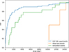 |
Fig. 11. CDFs of 90% localization areas for the O4b GW events (blue), simulated events (green), and observed AGN flare associations (orange). The median localization areas are 545 deg2 for the O4b events, 2300 deg2 for the simulated sample, and 11 590 deg2 for the observed sample. |
In addition to the Poisson and KS tests, we performed a Mood median test to compare the central tendency of the detection area distributions between simulations and observations. The test yielded a p-value of 0.26, indicating no statistically significant difference in the median detection areas.
5.3. Recovering BH merger triggered flares
We now considered the case in which all GW events trigger an AGN flare, and we investigated whether their optical counterparts would be detected. To do this, we used the GW event distance and chirp mass (available only for O4a) to estimate the expected apparent magnitude of the flare.
Using the O4 gravitational-wave transient catalog (The LIGO Scientific Collaboration et al. 2025), we obtained the chirp masses of the reported binary mergers in O4a and estimated their corresponding kick velocities that arose due to mass asymmetry (assuming no spin) from Equation (4) in Baker et al. (2008), approximated as
 (1)
(1)
where vkick is the kick velocity (in km s−1), η is the symmetric mass ratio  , A = 1.35 × 10⁴ km s−1, and B = −1.74. The optical luminosity of the kicked remnant was then computed using Equation (3) in Graham et al. (2023), which was subsequently converted into AB magnitudes.
A similar simulation was performed following the same procedure as above, with the modification that the flaring AGN distance distribution was now sampled from the luminosity-distance distributions of the GW events. Each sampled event was assigned a realistic apparent magnitude, mAB, and the detection threshold was imposed based on the limiting magnitude of ZTF. When assigning an apparent magnitude, we assumed an AGN disk density of 10−10 g cm−3 as in Graham et al. (2023). Under the previous assumption, all of the GW triggered flares would have been detected in O4a.
To summarize, we initially evaluated the likelihood of random associations using a Poisson test. This indicated that the single event detected during the O4a run might plausibly be a random association, whereas the four events detected during O4b might correspond to real physical connections.
To further investigate the O4b case, in particular, their large sky-map areas, we applied KS and Moore median tests. The simulated and observed events are consistent with being drawn from the same underlying distribution. This implies that the sky-map areas seen in the distribution of observed events are not significantly larger than those from the simulations.
Additionally, if AGN accretion disk gas densities are < 10−10 g cm−3 and recoil velocities dominated by mass asymmetry, our simulations indicate that when all these events occur within an AGN disk, they would be detectable.
6. Discussion
We developed an algorithm using the ALeRCE infrastructure. Upon receiving GW sky maps, the algorithm applies a sequence of spatial, temporal, and probabilistic filters to identify promising electromagnetic counterpart candidates. We applied this algorithm to multidetector GW superevents from the O4a and O4b observing runs. It identified one and four interesting candidates, respectively. Several of these candidates have already been reported to the TNS, although they remain unclassified. Two of the four events lie in the overlapping regime of SN and TDE (ZTF24abricne, ZTF24absmrlr); one event lies in the TDE regime (ZTF25aafwffi), and two events lie in the AGN regime (ZTF23abqkwzr, ZTF25aagpypz), as defined in Figure 2 of Graham et al. (2023).
To place the inferred AGN disk parameters (Table 3) in the context of AGN disk theory, we note that the derived scale heights, H/Rg ∼ 0.8 − 50 for SMBH masses of 107.1 − 108.4 M⊙, were obtained using the maximum recoil velocities, and they therefore represent upper limits on the disk thickness. Most values (H/Rg ≲ 10) are consistent with the thin or moderately thick regions of AGN accretion disks predicted by analytic models (e.g., Sirko & Goodman 2003; Thompson et al. 2005), which yield H/R ∼ 10−2 − 0.3 for the inner to self-gravitating disk regimes. The few higher ratios likely either reflect the assumption of maximum kick velocities or local disk inflation. Overall, the inferred geometries, even as upper limits, are broadly consistent with the vertical structures expected for AGN disks, supporting an origin of these flares within the inner or moderately thick disk regions. If the recoil velocity can be independently constrained from GW data (Varma et al. 2019, 2020), this approach could be used to estimate the disk density of the corresponding AGN accretion disk.
We also estimated the expected number of optical counterparts arising from random flare associations within ZTF alerts during the O4a and O4b runs. This estimate, shown as a function of GW sky-map threshold area in Figure 10, provides a baseline for interpreting the statistical significance of our detections. The observed excess, in the context of the observed event areas being larger than the median GW sky-map areas (as shown in 4), suggests a random association in O4a, whereas the four events detected during O4b might correspond to real physical connections.
As suggested by Graham et al. (2023) and demonstrated in Cabrera et al. (2024), genuine counterparts are expected to exhibit spectra consistent with an off-center explosive event, potentially producing asymmetric broad-line components. However, the O4a candidate shows no such asymmetry in its broad-line profile, and for the O4b candidates, we were unable to test this spectroscopically because the flare timescales were shorter and the events were identified well after their peak activity. While some of these sources might represent false positives, the use of the nuclear transient classifier helped us to mitigate this risk by selecting variability associated with AGN.
6.1. Implications for upcoming observing runs
Our algorithm was designed within the ALeRCE alert broker framework, but can be readily adapted for use with other brokers when similar classification probabilities are provided. Running it at least once per month during future observing runs would allow us to detect transients during their rising phase. Leveraging the ALeRCE watchlist7 feature enables continuous tracking of high-priority GW counterpart candidates, facilitating timely spectroscopic follow-up. This approach provides an efficient survey-based means to identify potential electromagnetic counterparts to GW events with large localization areas, which is particularly valuable when dedicated follow-up facilities are limited. Thus, our method offers a complementary route for capturing transient candidates that might otherwise be missed.
6.2. Comparison with other studies
Cabrera et al. (2024) reported a probable electromagnetic counterpart to the GW event S230922g based on dedicated follow-up observations. Since this source lies too far south to be observed by ZTF, its location likely explains why our search did not recover the candidate. Sun et al. (2025) discussed the possibility of a repeated partial TDE, that is, AT2021aeuk being a result of a stellar mass merger within the accretion disk that might produce similar phenomena.
Darc et al. (2025) outlined a framework for long-term optical monitoring of BBH events, while Zhang et al. (2025) emphasized coordination between wide-field imagers and multi-object spectrographs to maximize multimessenger yield.
More recently, Cabrera et al. (2025) statistically expanded upon the results of Graham et al. (2023), demonstrating that fewer than 3% of BBH mergers are likely to produce an observable optical counterpart. This implies that up to ∼40% of BBH mergers might occur within AGN accretion disks, although only a small fraction would yield detectable flares. These findings are broadly consistent with our results, where approximately 1 out of 70 events in the O4a run and 3 out of 105 events in the O4b run exhibited potential optical counterparts.
Furthermore, Cabrera et al. (2025) found no compelling evidence that higher-mass mergers are preferentially associated with AGN flares, suggesting that the apparent excess of high-mass events reported by Graham et al. (2023) may instead arise from chance coincidences. Our analysis explores around the scenario that the AGN flares might be linked to lower chirp mass and distant mergers, a scenario that remains compatible with the inferred occurrence rates.
7. Conclusions
Establishing a robust association between LVK GW events and possible optical flare counterparts remains a significant challenge in the pursuit of identifying BBH-EM counterparts. Because such transients occupy a region in the parameter space that overlaps with TDEs and other NTs, the development of improved theoretical models and time-dependent simulations for slowly evolving transients is essential. Dedicated follow-up campaigns of LVK events, such as those presented in Cabrera et al. (2024), are critical for advancing this effort.
We have developed an algorithm that leverages the ALeRCE infrastructure to systematically search for optical counterparts to GW superevents detected during the LVK O4a and O4b observing runs. The search yielded five promising candidates, one of which was previously reported as AT2023zgo on the TNS, while the remaining sources are yet to be conclusively classified.
We found a modest excess of AGN flares that are spatially and temporally coincident with GW localizations compared to random expectations, particularly during the O4b observing run. These coincidences predominantly occur in superevents with large localization areas where random overlaps are most likely, however. Our algorithm is specifically designed to efficiently identify potential associations over such extended regions, providing sensitivity to counterparts that may otherwise remain undetected. Statistical comparisons between the observed and simulated samples using KS and Mood median tests yield no significant differences, indicating that the observed events are statistically consistent with expectations for genuine AGN–GW associations. Overall, the evidence remains suggestive rather than definitive, underscoring the need for larger samples, improved localization, and detailed multiwavelength follow-up to confirm or refute a physical connection between AGN flares and GW events.
Nonetheless, our method remains highly effective in probing large sky areas that are typically inaccessible to targeted telescope follow-up. By statistically prioritizing AGN candidates based on probabilistic consistency rather than a brute force approach, this approach provides a complementary path to GW EM counterpart searches.
Furthermore, the imminent dissemination of public alert streams from LS4 (Miller et al. 2025) and the Vera C. Rubin Observatory (LSST, Ivezić et al. 2019) will dramatically expand the discovery space for optical transients. The resulting increase in event volume will significantly enhance the prospects for identifying optical counterparts to BBH mergers and for performing systematic population-level studies of NTs that might be associated with GW sources. In this context, our framework provides a baseline and statistically driven foundation for prioritizing multimessenger candidates in real time, ensuring readiness for the high-cadence, data-rich environment of forthcoming survey facilities. Further scalability tests need to performed, however.
Data availability
All source codes and trained models used in this work (apart from nuclear transients classifier, which will be available in a future publication) are publicly available. The ALeRCE stamp and light-curve classifiers were not implemented in this work, we obtained the corresponding classification probabilities from the ALeRCE database using the direct SQL access. The ALeRCE pipeline repository is found in GitHub8. The GW–AGN Watcher framework, including the cross-matching pipeline and chirp-mass prediction algorithm, is available in GitHub9, archived at Zenodo10and also as a pip installable package11. This repository includes documentation, example notebook, AGN catalog and configuration files required to reproduce the results presented in this paper.
Acknowledgments
Thanks to Amrita Singh for comments and help reading the manuscript. H.B. acknowledges the financial support from ANID NATIONAL SCHOLARSHIPS/DOCTORATE 21241862. F.F. and H.B. acknowledge support from ANID BASAL Project CATA (FB210003). A.M.A., F.F. and H.B. acknowledge support from ANID BASAL Project CMM (FB210005). A.M.A., F.F., H.B. and M.L.M.A. acknowledge support from ANID Millennium Science Initiative MAS (AIM23-0001). L.H.G. acknowledges financial support from ANID program FONDECYT Iniciación 11241477. M.L.M.A. and L.H.G. acknowledge support from ANID Millennium Science Initiative TITANS (NCN202_002). M.L.M.A. acknowledges support from the China-Chile Joint Research Fund (CCJRF2310). This research made use of Astropy (Astropy Collaboration 2013, 2018, 2022), HEALPix (Górski et al. 2005), ligo.sky map (Singer & Price 2016), Matplotlib (Hunter 2007), NumPy (Harris et al. 2020), Pandas (pandas development team 2020), PostgreSQL (PostgreSQL Global Development Group 2022), SciPy (Virtanen et al. 2020), Scikit-learn (Pedregosa et al. 2011), alphashape (Bellock 2021), ALeRCE (Förster et al. 2021), gracedb-sdk (Singer 2022), pesummary (Hoy & Raymond 2021), and Q3C (Koposov & Bartunov 2006). We also used data and software from the Zwicky Transient Facility (ZTF) (Bellm et al. 2018), the LIGO–Virgo–KAGRA Collaboration (LVK) (Abbott et al. 2016) observing runs and sky localizations.
References
- Abbott, B. P., Abbott, R., Abbott, T. D., et al. 2016, Phys. Rev. Lett., 116, 061102 [Google Scholar]
- Abbott, R., Abbott, T. D., Acernese, F., et al. 2023, Phys. Rev. X, 13, 011048 [NASA ADS] [Google Scholar]
- Abbott, R., Abbott, T. D., Acernese, F., et al. 2024, Phys. Rev. D, 109, 022001 [NASA ADS] [CrossRef] [Google Scholar]
- Agayeva, S., Aivazyan, V., Alishov, S., et al. 2022, Proc. SPIE, submitted [arXiv:2207.10178] [Google Scholar]
- Astropy Collaboration (Robitaille, T. P., et al.) 2013, A&A, 558, A33 [NASA ADS] [CrossRef] [EDP Sciences] [Google Scholar]
- Astropy Collaboration (Price-Whelan, A. M., et al.) 2018, A&A, 620, A203 [NASA ADS] [CrossRef] [EDP Sciences] [Google Scholar]
- Astropy Collaboration (Price-Whelan, A. M., et al.) 2022, ApJ, 935, 167 [NASA ADS] [CrossRef] [Google Scholar]
- Baker, J. G., Boggs, W. D., Centrella, J., et al. 2008, ApJ, 682, L29 [NASA ADS] [CrossRef] [Google Scholar]
- Bartos, I., Kocsis, B., Haiman, Z., & Márka, S. 2017, ApJ, 835, 165 [Google Scholar]
- Belczynski, K., Klencki, J., Fields, C. E., et al. 2020, A&A, 636, A104 [NASA ADS] [CrossRef] [EDP Sciences] [Google Scholar]
- Bellm, E. C., Kulkarni, S. R., Graham, M. J., et al. 2018, PASP, 131, 018002 [Google Scholar]
- Bellock, K. 2021, alphashape: Toolbox for constructing alpha shapes (GitHub) [Google Scholar]
- Bentz, M. C., Denney, K. D., Grier, C. J., et al. 2013, ApJ, 767, 149 [Google Scholar]
- Boroson, T. A., & Green, R. F. 1992, ApJS, 80, 109 [Google Scholar]
- Bowen, I. S. 1928, ApJ, 67, 1 [Google Scholar]
- Burrows, D. N., Hill, J. E., Nousek, J. A., et al. 2005, Space Sci. Rev., 120, 165 [Google Scholar]
- Cabrera, T., Palmese, A., Hu, L., et al. 2024, Phys. Rev. D, 110, 123029 [Google Scholar]
- Cabrera, T., Palmese, A., & Fishbach, M. 2025, arXiv e-prints [arXiv:2510.20767] [Google Scholar]
- Cappellari, M. 2017, MNRAS, 466, 798 [Google Scholar]
- Cappellari, M. 2023, MNRAS, 526, 3273 [NASA ADS] [CrossRef] [Google Scholar]
- Cardelli, J. A., Clayton, G. C., & Mathis, J. S. 1989, ApJ, 345, 245 [Google Scholar]
- Carrasco-Davis, R., Reyes, E., Valenzuela, C., et al. 2021, AJ, 162, 231 [NASA ADS] [CrossRef] [Google Scholar]
- Cartier, R., Contreras, C., Stritzinger, M., et al. 2026, A&A, 707, A161 [NASA ADS] [CrossRef] [EDP Sciences] [Google Scholar]
- Chambers, K. C., Magnier, E. A., Metcalfe, N., et al. 2016, arXiv e-prints [arXiv:1612.05560] [Google Scholar]
- Coughlin, M. W., Bloom, J. S., Nir, G., et al. 2023, ApJS, 267, 31 [NASA ADS] [CrossRef] [Google Scholar]
- Cutri, R. M., Wright, E. L., Conrow, T., et al. II/328., 002021. VizieR On-line Data Catalog [Google Scholar]
- Darc, P., Bom, C. R., Kilpatrick, C. D., et al. 2025, Phys. Rev. D, 112, 063019 [Google Scholar]
- Evans, P. A., Page, K. L., Beardmore, A. P., et al. 2023, MNRAS, 518, 174 [Google Scholar]
- Flesch, E. W. 2023, OJAp, 6, 49 [NASA ADS] [Google Scholar]
- Ford, K. E. S., & McKernan, B. 2022, MNRAS, 517, 5827 [NASA ADS] [CrossRef] [Google Scholar]
- Förster, F., Cabrera-Vives, G., Castillo-Navarrete, E., et al. 2021, AJ, 161, 242 [CrossRef] [Google Scholar]
- Gerosa, D., & Fishbach, M. 2021, Nat. Astron., 5, 749 [NASA ADS] [CrossRef] [Google Scholar]
- Gilbaum, S., Grishin, E., Stone, N. C., & Mandel, I. 2025, ApJ, 982, L13 [Google Scholar]
- Gomez, S., Villar, V. A., Berger, E., et al. 2023, ApJ, 949, 113 [Google Scholar]
- Górski, K. M., Hivon, E., Banday, A. J., et al. 2005, ApJ, 622, 759 [Google Scholar]
- Graham, M., Ford, K., McKernan, B., et al. 2020, Phys. Rev. Lett., 124, 251102 [NASA ADS] [CrossRef] [Google Scholar]
- Graham, M. J., McKernan, B., Ford, K. E. S., et al. 2023, ApJ, 942, 99 [Google Scholar]
- Greene, J. E., & Ho, L. C. 2005, ApJ, 630, 122 [NASA ADS] [CrossRef] [Google Scholar]
- Gröbner, M., Ishibashi, W., Tiwari, S., Haney, M., & Jetzer, P. 2020, A&A, 638, A119 [NASA ADS] [CrossRef] [EDP Sciences] [Google Scholar]
- Gromadzki, M., Hamanowicz, A., Wyrzykowski, L., et al. 2019, A&A, 622, L2 [NASA ADS] [CrossRef] [EDP Sciences] [Google Scholar]
- Harris, C. R., Millman, K. J., van der Walt, S. J., et al. 2020, Nature, 585, 357 [NASA ADS] [CrossRef] [Google Scholar]
- Herner, K., Annis, J., Brout, D., et al. 2020, Astron. Comput., 33, 100425 [Google Scholar]
- Hosseinzadeh, G., Paterson, K., Rastinejad, J. C., et al. 2024, ApJ, 964, 35 [Google Scholar]
- Hoy, C., & Raymond, V. 2021, SoftwareX, 15, 100765 [Google Scholar]
- Hunter, J. D. 2007, Comput. Sci. Eng., 9, 90 [NASA ADS] [CrossRef] [Google Scholar]
- IceCube Collaboration. 2019, GCN, 26258, 1 [Google Scholar]
- Ihanec, N., Petrushevska, T., Gromadzki, M., & Yaron, O. 2024, TNS Classif. Rep., 2024-97, 1 [Google Scholar]
- Ivezić, Ž., Kahn, S. M., Tyson, J. A., et al. 2019, ApJ, 873, 111 [Google Scholar]
- Kimura, S. S., Murase, K., & Bartos, I. 2021, ApJ, 916, 111 [Google Scholar]
- Koposov, S., & Bartunov, O. 2006, ASPC, 351, 735 [Google Scholar]
- Kunnumkai, K., Palmese, A., Cabrera, T., et al. 2024, AAS Meet. Abstr., 243, 324.06 [Google Scholar]
- Leloudas, G., Dai, L., Arcavi, I., et al. 2019, ApJ, 887, 218 [NASA ADS] [CrossRef] [Google Scholar]
- Makrygianni, L., Trakhtenbrot, B., Arcavi, I., et al. 2023, ApJ, 953, 32 [NASA ADS] [CrossRef] [Google Scholar]
- Malyali, A., Rau, A., Merloni, A., et al. 2021, A&A, 647, A9 [NASA ADS] [CrossRef] [EDP Sciences] [Google Scholar]
- Mapelli, M. 2020, Front. Astron. Space Sci., 7, 38 [NASA ADS] [CrossRef] [Google Scholar]
- Masci, F. J., Laher, R. R., Rusholme, B., et al. 2019, PASP, 131, 018003 [Google Scholar]
- Masci, F. J., Laher, R. R., Rusholme, B., et al. 2023, arXiv e-prints [arXiv:2305.16279] [Google Scholar]
- Matheson, T., Stubens, C., Wolf, N., et al. 2021, AJ, 161, 107 [NASA ADS] [CrossRef] [Google Scholar]
- McKernan, B., Ford, K. E. S., Lyra, W., & Perets, H. B. 2012, MNRAS, 425, 460 [NASA ADS] [CrossRef] [Google Scholar]
- McKernan, B., Ford, K. E. S., Bellovary, J., et al. 2018, ApJ, 866, 66 [Google Scholar]
- Mejía-Restrepo, J. E., Lira, P., Netzer, H., Trakhtenbrot, B., & Capellupo, D. M. 2018, Nat. Astron., 2, 63 [CrossRef] [Google Scholar]
- Miller, A. A., Abrams, N. S., Aldering, G., et al. 2025, PASP, 137, 094204 [Google Scholar]
- Möller, A., Peloton, J., Ishida, E. E. O., et al. 2021, MNRAS, 501, 3272 [CrossRef] [Google Scholar]
- pandas development team, T. 2020, https://doi.org/10.5281/zenodo.3509134 [Google Scholar]
- Pavez-Herrera, M., Sánchez-Sáez, P., Hernández-García, L., et al. 2025, A&A, 696, A153 [NASA ADS] [CrossRef] [EDP Sciences] [Google Scholar]
- Pedregosa, F., Varoquaux, G., Gramfort, A., et al. 2011, JMLR, 12, 2825 [Google Scholar]
- Perna, R., Lazzati, D., & Cantiello, M. 2021, ApJ, 906, L7 [Google Scholar]
- Petrov, P., Singer, L. P., Coughlin, M. W., et al. 2022, ApJ, 924, 54 [NASA ADS] [CrossRef] [Google Scholar]
- PostgreSQL Global Development Group. 2022, PostgreSQL v14.6, https://www.postgresql.org/ [Google Scholar]
- Rau, M. M., Seitz, S., Brimioulle, F., et al. 2015, MNRAS, 452, 3710 [NASA ADS] [CrossRef] [Google Scholar]
- Reines, A. E., Greene, J. E., & Geha, M. 2013, ApJ, 775, 116 [Google Scholar]
- Rodríguez-Ramírez, J. C., Nemmen, R., & Bom, C. R. 2025, Phys. Rev. D, 111, 083020 [Google Scholar]
- Roming, P. W. A., Kennedy, T. E., Mason, K. O., et al. 2005, Space Sci. Rev., 120, 95 [Google Scholar]
- Russeil, E., Malanchev, K. L., Aleo, P. D., et al. 2024, A&A, 683, A251 [NASA ADS] [CrossRef] [EDP Sciences] [Google Scholar]
- Samsing, J., Bartos, I., D’Orazio, D. J., et al. 2022, Nature, 603, 237 [NASA ADS] [CrossRef] [Google Scholar]
- Sánchez-Sáez, P., Reyes, I., Valenzuela, C., et al. 2021, AJ, 161, 141 [CrossRef] [Google Scholar]
- Singer, L. 2022, gracedb-sdk v0.1.7, https://git.ligo.org/emfollow/gracedb-sdk [Google Scholar]
- Singer, L. P., & Price, L. R. 2016, Phys. Rev. D, 93, 024013 [CrossRef] [Google Scholar]
- Sirko, E., & Goodman, J. 2003, MNRAS, 341, 501 [NASA ADS] [CrossRef] [Google Scholar]
- Śniegowska, M., Trakhtenbrot, B., Makrygianni, L., et al. 2025, arXiv e-prints [arXiv:2505.00083] [Google Scholar]
- Soni, S., Berger, B. K., Davis, D., et al. 2025, Class. Quant. Grav., 42, 085016 [Google Scholar]
- Sun, J., Guo, H., Gu, M., et al. 2025, ApJ, 982, 150 [Google Scholar]
- Tadhunter, C., Spence, R., Rose, M., Mullaney, J., & Crowther, P. 2017, Nat. Astron., 1, 0061 [NASA ADS] [CrossRef] [Google Scholar]
- Tagawa, H., Haiman, Z., & Kocsis, B. 2020, ApJ, 898, 25 [NASA ADS] [CrossRef] [Google Scholar]
- Tagawa, H., Kocsis, B., Haiman, Z., et al. 2021, ApJ, 908, 194 [NASA ADS] [CrossRef] [Google Scholar]
- Tagawa, H., Kimura, S. S., Haiman, Z., Perna, R., & Bartos, I. 2023, ApJ, 946, L3 [NASA ADS] [CrossRef] [Google Scholar]
- The LIGO Scientific Collaboration, the Virgo Collaboration,& the KAGRA Collaboration, et al. 2025, arXiv e-prints [arXiv:2508.18082] [Google Scholar]
- Thompson, T. A., Quataert, E., & Murray, N. 2005, ApJ, 630, 167 [Google Scholar]
- Tonry, J. L., Denneau, L., Heinze, A. N., et al. 2018, PASP, 130, 064505 [Google Scholar]
- Trakhtenbrot, B., Arcavi, I., Ricci, C., et al. 2019, Nat. Astron., 3, 242 [Google Scholar]
- Vanden Berk, D. E., Richards, G. T., Bauer, A., et al. 2001, AJ, 122, 549 [Google Scholar]
- Varma, V., Field, S. E., Scheel, M. A., et al. 2019, Phys. Rev. Res., 1, 033015 [NASA ADS] [CrossRef] [Google Scholar]
- Varma, V., Isi, M., & Biscoveanu, S. 2020, Phys. Rev. Lett., 124, 101104 [NASA ADS] [CrossRef] [Google Scholar]
- Vazdekis, A., Koleva, M., Ricciardelli, E., Röck, B., & Falcón-Barroso, J. 2016, MNRAS, 463, 3409 [Google Scholar]
- Veitch, J., Raymond, V., Farr, B., et al. 2015, Phys. Rev. D, 91, 042003 [NASA ADS] [CrossRef] [Google Scholar]
- Veres, P. M., Franckowiak, A., van Velzen, S., et al. 2026, A&A, 706, A324 [NASA ADS] [CrossRef] [EDP Sciences] [Google Scholar]
- Veronesi, N., van Velzen, S., & Rossi, E. M. 2024, MNRAS, 536, 3112 [Google Scholar]
- Virtanen, P., Gommers, R., Oliphant, T. E., et al. 2020, Nat. Methods, 17, 261 [Google Scholar]
- Wang, J.-M., Liu, J.-R., Ho, L. C., Li, Y.-R., & Du, P. 2021, ApJ, 916, L17 [Google Scholar]
- Zhang, H., Kokubo, M., MacBride, S., et al. 2025, ApJ, submitted [arXiv:2508.00291] [Google Scholar]
The chirp mass information is circulated in the GCN circulars from June 2025 in the form of a probability distribution in the mass range bins.
 , where λ0 is the rest-frame wavelength, λR(x) and λB(x) are the red and blue wavelengths at
  ,
,  , and c is the speed of light.
fBLR = (FWHMHβ / 4550±1000)−1.17

Appendix A: Chirp mass prediction
This section contains plots representing testing and validation results of our chirp mass prediction algorithm for O3 merger events
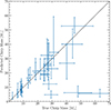 |
Fig. A.1. Performance of the algorithm on GW events from the third LVK observing run (O3) (Abbott et al. 2023); abbott.2024. The X axis denotes the chirp mass inferred using LALInference (Veitch et al. 2015) parameter estimation and the Y axis represents masses predicted by our OCP algorithm. These estimations were made using an identical number of BAYESTAR simulations made with the actual O3 detector noise curves. Poor estimation in the low mass region can be attributed to variability in the stability of detector noise curves. |
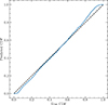 |
Fig. A.2. P-P plot of predicted chirp mass vs true chirp mass of simulated events. The black dashed line represents ideal situation with no bias, while blue line represents the pp curve of the algorithm. The distributions are similar to each other, with small bias occurring at the edges of the distribution. |
Appendix B: Multiwavelength follow up of AT 2023zgo
In this section, we present the multiwavelength follow-up and analysis of the event AT2023zgo. The optical light curve was tested for consistency with a TDE using a power-law decay fit. However, as shown in Fig. B.1, the best-fitting power-law model does not reproduce the observed evolution, indicating that AT 2023zgo is inconsistent with a TDE interpretation.
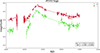 |
Fig. B.1. Fitting the light curve with a power-law decay model(TDE) with reference to Pavez-Herrera et al. (2025). The a power law index fit values are of 0.518 ±0.0118 for g-band and 0.389 ± 0.0082 for r-band in contrast to -1.66 expected for a TDE. |
Given the uniqueness of the flare and its potential association with a binary black hole (BBH) merger, we examined the source for emission in the ultraviolet (UV) and X-ray regimes to search for possible jet-related signatures, as relativistic jets have been proposed in BBH merger environments (Tagawa et al. 2023). The follow-up observations for other potential counterpart candidates were not feasible due to the short timescale and rapid decline of those transient events. Future coordinated multiwavelength campaigns will be essential to confirm the physical nature of Bowen-type flares and to distinguish them from other classes of AGN-related transients.
B.1. Bowen fluorescence lines
Trakhtenbrot et al. (2019) described the discovery of the transient optical event AT 2017bgt, which was observed in the nucleus of the early-type galaxy 2MASX J16110570+0234002, at z = 0.064. This event was characterized by an unusual optical flare and the appearance of Bowen fluorescence flares (BFF) in its spectrum. The authors suggested that the SMBH experienced a sudden increase in their UV-optical emission.
When high-energy UV radiation from a central source, like a supermassive black hole in an AGN, ionizes atoms or ions in the surrounding gas, this process excites the gas, causing it to emit light as it returns to lower energy states. Specifically, the photons ionize helium (He II λ304Å), which then induces a cascade of electronic transitions in ions such as O III (with emission lines around λ3133 Å) and N III (with emission lines around λ4634 Å, λ4641 Å), producing distinctive emission lines known as Bowen fluorescence (Bowen 1928).
Makrygianni et al. (2023) presented a multiwavelength analysis of AT 2021loi, which showed the first clear evidence of a rebrightening after around one year after the first flare in a BFF. This source shows an optical rise of a factor four in about one month, and a slow decline of 13 months, and then the rebrightening after 400 days. They discussed that the event could be related to an increase in the Eddington rate.
AT 2019aalc is another BFF that showed a first peak in 2019, and a rebrightening in 2023 (Veres et al. 2026; Śniegowska et al. 2025). The rebrightening indeed showed stronger flux increase than the first peak, strong and broad (∼2000 km s−1) He II λ4686Å and N III λ4640Å lines, a slow decay of the light curve in general agreement with other BFFs. The first peak was coincident with a neutrino event (IC 191119A IceCube Collaboration 2019). Śniegowska et al. (2025) discussed that the origin of the BFF could be related to radiation pressure instabilities in the (pre-existing) accretion disk of an AGN.
Other sources that have been related to the BFF family are F01007 (Tadhunter et al. 2017), OGLE17aaj (Gromadzki et al. 2019), and AT2019avd (Malyali et al. 2021).
One curious property of almost all these systems is that they occurred in Narrow Line Seyfert 1 (NLSy1) galaxies.
BFFs have also been observed in TDEs (e.g., Leloudas et al. 2019), but their properties seem to differ from these BFF systems, which show slow decline in their light curves, a rebrightening after years, the absence of very broad He II λ4686Å (> 10000 km s−1), and have preference to occur in AGN.
B.2. Spectroscopic observations
Light curves and spectra play a fundamental role in distinguishing among the diverse transient events observed in AGNs, including tidal disruption events and changing-look events. In light of the peculiar characteristics of the transient AT2023zgo, as reported in the TNS, we conducted a Target-of-Opportunity (ToO) spectroscopic follow-up using the SOAR Goodman spectrograph (Program ID: SOAR2025A-027, PI: H. Bommireddy). To obtain full coverage of the optical wavelength range, we employed the Goodman Red configuration in the 400 M1 and 400 M2 modes, with a total exposure time of 1200 s per configuration. Arc lamp and spectrophotometric standard star calibrations were acquired with the science observations. The two-dimensional Goodman spectra were reduced using standard steps, including bias removal, flat-field correction, and wavelength calibration using NeArHg lamps. The wavelength calibration was checked against sky emission lines. The one-dimensional spectra were optimally extracted and then flux-calibrated using a flux standard observed immediately after the science spectra (see Cartier et al. 2026), for more details). The resulting spectra is shown in green in Figure B.2.
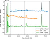 |
Fig. B.2. AT2023zgo spectroscopic follow-up observations - Bowen fluorescence lines OIII(3133Å), HeII(4696Å), NIII(4640Å) overplotted against candidate of GW event S230630bq (+130d pm) |
The archival spectra (in blue) of the host galaxy was retrieved from SDSS DR17 (MJD: 52991), the reported spectrum in TNS as on peak brightness ( 70 days after detection - MJD 60318) of the event with NTT (Ihanec et al. 2024), and with SOAR (∼400 days after detection - MJD 60699)
B.3. Fitting of optical spectra
Spectra were corrected for Galactic extinction following the law of Cardelli et al. (1989) and later corrected by redshift (z = 0.23296). In the spectral fitting model includes contributions from the accretion disk (modeled as a power-law), the stellar population, iron pseudo-continuum (Boroson & Green 1992) and all emission lines reported by Vanden Berk et al. (2001) plus the Bowen Fluorescence line NIIIλ4640. Among the three available spectra, the SDSS observation corresponds to the dimmer AGN activity. We therefore used this spectrum to model the stellar contribution, employing the pPXF code (Cappellari 2017) and the E-MILES stellar population (SSP) templates (Vazdekis et al. 2016). Given that the stellar component evolves on timescales higher than 106 years, it was fixed in the spectral fitting of the NTT and SOAR observations, allowing only the powerlaw component to vary. All the emission lines were modeled with Gaussian profiles, and a double Gaussian profile was considered to reproduce the broad and narrow components, as in the case of the Balmer lines. The final spectral fitting was obtained using a MCMC-based fitting code employed in previous AGN studies.
The equivalent widths (W) and the Full Width at Half Maximum (FWHM) of the most important emission lines are reported in Tab. B.1, while a comparison of the relevant spectral regions (after continuum subtraction) is shown in Fig. B.3.
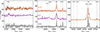 |
Fig. B.3. Comparison of the relevant spectral regions after continuum subtraction for each observation. A constant factor has been added to the NTT (+30) and SOAR (+60) spectra for visualization purposes. Dashed line correspond to the total fitting. The vertical lines indicates the wavelength rest-frame of the emission lines. |
Emission line properties
We found that the power-law becomes steeper in the NTT and SOAR spectra, indicating a significant increment in the UV ionizing continuum flux and the appearance of the Balmer bump in the spectrum after the flare. This coincides with the remarkable increment in the equivalent widths of the Balmer lines for the NTT and SOAR observations compared to the dimmer state (SDSS spectra). The detection of the Bowen fluorescence emission lines such as OIIIλ3133 and NIIIλ4640, as well as high ionization lines like HeIIλ4685 and HeI3188, also support the presence of a harder UV continuum in the post-flare spectra. The FWHM measured for OIIIλ3133 and NIIIλ4640 is similar to the one found in the Balmer Lines (2000-3000 km s−1). This suggests that the Bowen Fluorescence emission lines originate also in the broad line region (BLR).
To model the Hα emission line in the SOAR spectrum, we included a second broad Gaussian profile to reproduce the base of the emission line. This component shows an equivalent width of 75.1±4.1 Å and a FWHM of 6,954±75 km s−1. Considering both components, the FWHM of the total profile is 2049±112 km s−1. We also include a second broad component in the Hβ profile, however, its contribution is negligible. The physical meaning of a second component in the Hα profile would indicate an increment in the velocity dispersion of the BLR gas or the presence of outflows. We measure the velocity centroid12 (cx) at different level of the profile investigate possible asymmetries, a key indicator of a BBH merger. The velocity centroid is ∼30 km s−1 at different levels of the profile, corresponding to a shift of < 1 Å with respect to the Hα rest-frame. This indicates that the full Hα profile is completely symmetric and rule out the presence of any outflow. So, we conclude that the third broad component corresponds to an increment in the velocity dispersion of the BLR.
Table B.1 lists the bolometric luminosity, black hole mass and Eddington ratio. The luminosity of the AGN at 5100Å is estimated from the powerlaw fitting.
We obtained the black hole mass through the classical relation MBH = fBLR ⋅ RBLR ⋅ v2/G, where G is the gravitational constant, fBLR is the virial factor13 (Mejía-Restrepo et al. 2018), RBLR is the size of the broad line region obtained from the Hβ Radius-Luminosity14 (Bentz et al. 2013), and v is the the velocity field of the broad line region represented by the FWHM of Hβ. The black hole mass for the observations is similar within uncertainties with a median value of 7.7 M⊙. The Eddington ratio increases by a factor of 1.7 in the NTT and SOAR spectra with respect to the SDSS observation. This confirms the presence of a hard UV continuum in the post-flare observations.
The convolution between the accretion disk and host galaxy contributions could carry out uncertainties on the continuum flux and then in the black hole mass and Eddington ratio estimations. Alternatively, the black hole mass can be estimated with the luminosity and FWHM of the Hα emission lines following the description of Reines et al. (2013). We obtained a black hole mass of 7.4±0.05 M⊙ and 7.4±0.06 M⊙ for the SDSS and SOAR spectra. These values are 0.2-0.4 dex compared with the black hole mass estimated from continuum luminosity.
The source is cataloged as a Narrow Line Seyfert 1 (NLS1) according to the flux ratio [OIII λ5007]/Hβ = 0.9. In a BPT diagram, the target is located in the transition region between starforming and LINERs. This means that the ionizing radiation comes from the AGN plus young stars.
B.4. Neil Gehrels Swift Observatory
The Swift X-ray Telescope (XRT, Burrows et al. 2005), onboard the Neil Gehrels Swift Observatory, observed AT2023zgo in the Photon Counting (PC) between January 17th and May 29th, 2024, approximately once per week, taking a total of 18 observations. The source was not detected on individual observations, and count rates and upper limits were retrieved from the living Swift-XRT point source catalog (Evans et al. 2023), and converted into flux using WebPIMMS and a power law model using a spectral index of 2 and galactic absorption 2.62×1020cm−2. The flux upper limits are in the range between 1.2×10⁻¹³ and 5.1×10⁻¹³ erg s−1cm−2. Stacking all the observations results in a 24 ksec observation and a 2σ detection with a flux of 1.1[0.4-1.7]×10−14 erg s−1cm−2.
The Ultraviolet and Optical Telescope (UVOT, Roming et al. 2005) observes simultaneously with the X-ray observations on each epoch. Observations were obtained with the six primary photometric filters: V (centered at 5468 Å), B (at 4392 Å), U (at 3465 Å), UVW1 (at 2600 Å), UVM2 (at 2246 Å) and UVW2 (at 1928 Å). The UVOTSOURCE task within software HEASoft version 6.33 was used to perform aperture photometry using a circular aperture of radius 5 arcsec centered on the coordinates of AT2023zgo. The background region was selected free of sources adopting a circular region of 20 arcsec close to the nucleus. There are certain areas in the UVOT detector where the throughput is lower than for the rest of the detector, so observations affected by this effect were not taken into account.
The ZTF light curve of AT2023zgo is presented in difference flux (i.e., the variable flux) in Fig. B.4, with the Swift/UVOT measurements in total flux, and in apparent magnitude (i.e., the magnitude corrected for the contribution of the host galaxy as measured in the reference image) in Fig. B.5, with the Swift/UVOT measurements in apparent magnitude. It is worth noting a very similar shape in this plot in the optical and UV data.
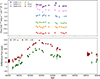 |
Fig. B.4. Swift/UVOT (in total flux) and ZTF forced photometry (in difference flux) data between September 13, 2023, and October 17, 2024. |
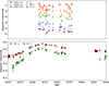 |
Fig. B.5. Swift/UVOT and ZTF forced photometry data in apparent magnitudes between September 13, 2023, and October 17, 2024. |
Appendix C: AGN spectra of counterpart candidates
Here we present the archival spectra before the onset of flare. This was essentially used for calculating the SMBH masses.
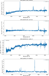 |
Fig. C.1. SDSS Archival spectra of the host AGNs for the counterpart candidates |
All Tables
ZTF events and corresponding GW superevents with location, light curve, and AGN properties.
All Figures
|
Fig. 1. Sky map from LVK of the GW event S240902bq. The color scale represents the probability contours. |
| In the text | |
|
Fig. 2. Sky map converted into bounded polygons (green boundaries) filled with ZTF public alerts in yellow. |
| In the text | |
|
Fig. 3. Distribution of classes by stamp classifier for the events originating with 1.4″ of the MQUAS AGN catalog for the O4a and O4b runs. |
| In the text | |
|
Fig. 4. Cumulative distribution function of the sky-map areas for O4a (top) and O4b (bottom) with median area values (vertical red lines). |
| In the text | |
|
Fig. 5. Total number of events for both runs, including all filters. |
| In the text | |
|
Fig. 6. Total number of events for both runs, excluding PS1 and location-based filter. |
| In the text | |
|
Fig. 7. Light curves of the O4a counterpart candidate AT2023zgo/ZTF23abqkwzr in ZTF g and r bands and g-r color for the science images and their forced photometry. The vertical line represents the GW event with which the corresponding ZTF alert might be associated. |
| In the text | |
|
Fig. 8. Light curves of O4b counterpart candidates in ZTF g and r bands and g-r color for the science images and their forced photometry. The vertical lines in each plot represent the time of the GW event. |
| In the text | |
|
Fig. 9. ZTF pointings for public alerts based on the quality assurance product for O4a (top) and O4b (bottom) with npointings ≥ 15, where the color scale represents the observation frequency. |
| In the text | |
|
Fig. 10. Cumulative distribution function of the simulated (blue) and detected flare events (red) corresponding to ZTF pointings up to 200 days post merger for each GW event as a function of GW sky-map area. The top panel corresponds to O4a, and the bottom panel corresponds to O4b. |
| In the text | |
|
Fig. 11. CDFs of 90% localization areas for the O4b GW events (blue), simulated events (green), and observed AGN flare associations (orange). The median localization areas are 545 deg2 for the O4b events, 2300 deg2 for the simulated sample, and 11 590 deg2 for the observed sample. |
| In the text | |
|
Fig. A.1. Performance of the algorithm on GW events from the third LVK observing run (O3) (Abbott et al. 2023); abbott.2024. The X axis denotes the chirp mass inferred using LALInference (Veitch et al. 2015) parameter estimation and the Y axis represents masses predicted by our OCP algorithm. These estimations were made using an identical number of BAYESTAR simulations made with the actual O3 detector noise curves. Poor estimation in the low mass region can be attributed to variability in the stability of detector noise curves. |
| In the text | |
|
Fig. A.2. P-P plot of predicted chirp mass vs true chirp mass of simulated events. The black dashed line represents ideal situation with no bias, while blue line represents the pp curve of the algorithm. The distributions are similar to each other, with small bias occurring at the edges of the distribution. |
| In the text | |
|
Fig. B.1. Fitting the light curve with a power-law decay model(TDE) with reference to Pavez-Herrera et al. (2025). The a power law index fit values are of 0.518 ±0.0118 for g-band and 0.389 ± 0.0082 for r-band in contrast to -1.66 expected for a TDE. |
| In the text | |
|
Fig. B.2. AT2023zgo spectroscopic follow-up observations - Bowen fluorescence lines OIII(3133Å), HeII(4696Å), NIII(4640Å) overplotted against candidate of GW event S230630bq (+130d pm) |
| In the text | |
|
Fig. B.3. Comparison of the relevant spectral regions after continuum subtraction for each observation. A constant factor has been added to the NTT (+30) and SOAR (+60) spectra for visualization purposes. Dashed line correspond to the total fitting. The vertical lines indicates the wavelength rest-frame of the emission lines. |
| In the text | |
|
Fig. B.4. Swift/UVOT (in total flux) and ZTF forced photometry (in difference flux) data between September 13, 2023, and October 17, 2024. |
| In the text | |
|
Fig. B.5. Swift/UVOT and ZTF forced photometry data in apparent magnitudes between September 13, 2023, and October 17, 2024. |
| In the text | |
|
Fig. C.1. SDSS Archival spectra of the host AGNs for the counterpart candidates |
| In the text | |
Current usage metrics show cumulative count of Article Views (full-text article views including HTML views, PDF and ePub downloads, according to the available data) and Abstracts Views on Vision4Press platform.
Data correspond to usage on the plateform after 2015. The current usage metrics is available 48-96 hours after online publication and is updated daily on week days.
Initial download of the metrics may take a while.