| Issue |
A&A
Volume 707, March 2026
|
|
|---|---|---|
| Article Number | A375 | |
| Number of page(s) | 13 | |
| Section | The Sun and the Heliosphere | |
| DOI | https://doi.org/10.1051/0004-6361/202557941 | |
| Published online | 24 March 2026 | |
Dynamics, thermodynamics, and fine structure of virtual erupting filaments
1
Centre for mathematical Plasma Astrophysics, Department of Mathematics, KU Leuven, Leuven, Belgium
2
School of Astronomy and Space Science and Key Laboratory of Modern Astronomy and Astrophysics, Nanjing University, Nanjing, PR China
3
Universidad de Mendoza, Mendoza, Argentina
⋆ Corresponding author: This email address is being protected from spambots. You need JavaScript enabled to view it.
Received:
2
November
2025
Accepted:
6
February
2026
Abstract
Context. It is not fully understood why some solar filaments erupt, whereas others do not. Filaments that erupt typically undergo a slow rise, followed by an acceleration phase; this transition requires further investigation. Erupting prominences have been observed to heat up during the acceleration phase, but the origin of this heating remains unclear. Moreover, some coronal mass ejections possess additional fine structure in white-light observations, in addition to the general three-structure morphology.
Aims. Our objective is to elaborate on the dynamics of erupting prominences, investigate why erupting filaments heat up in the acceleration phase, and correlate our findings with observations.
Methods. We used the open-source software tool MPI-AMRVAC to solve the 2.5D magnetohydrodynamic (MHD) equations on a coronal domain extending up to 300 Mm, using adaptive mesh refinement to achieve high resolution. We used controlled combinations of footpoint shearing and converging motions on an initial magnetic arcade to obtain erupting flux ropes, where self-consistent prominence and coronal rain formation occur due to thermal instability. We find both non-erupting and erupting cases, related to the energization of the system. We compared our erupting prominences with observations using data from the AIA Filament Eruption Catalog.
Results. We find that the slow rise and impulsive phases of erupting prominences are modulated by magnetic reconnection. The transition from slow rise to acceleration results from a change from a low inflow Alfvén Mach number to a higher one. For the first time, we demonstrate that thermal conduction and compressional heating can lead to prominence evaporation. We obtain clearly nested, circular fine structures in extreme ultraviolet images of the ejected flux ropes, already present during their early evolution in the low corona. Some of this structure results directly from upward-moving plasmoids that interact with the flux rope.
Conclusions. We conclude that thermal conduction and compressional heating are highly relevant heating mechanisms in erupting flux rope interiors, and that magnetic reconnection dictates the entire early evolution of coronal mass ejections, from the slow-rise phase to the impulsive phase.
Key words: Sun: corona / Sun: coronal mass ejections (CMEs) / Sun: filaments / prominences / Sun: magnetic fields
© The Authors 2026
 Open Access article, published by EDP Sciences, under the terms of the Creative Commons Attribution License (https://creativecommons.org/licenses/by/4.0), which permits unrestricted use, distribution, and reproduction in any medium, provided the original work is properly cited.
This article is published in open access under the Subscribe to Open model. This email address is being protected from spambots. You need JavaScript enabled to view it. to support open access publication.
1. Introduction
Solar prominences and filaments refer to the same coronal condensations, in which the density and temperature contrast with the ambient environment by around two orders of magnitude. It is now widely accepted that they are suspended by the magnetic field and that thermal instability plays a central role in their development (Parker 1953; Field 1965). Keppens et al. (2025) provide a review of prominence formation, covering theoretical insights from modeling efforts up to the current state of the art. Many numerical models exist to clarify their formation and subsequent dynamics; such models include the levitation–condensation model (Kaneko & Yokoyama 2017; Jenkins & Keppens 2021; Brughmans et al. 2022; Donné & Keppens 2024), the evaporation–condensation model (Zhou et al. 2014; Xia & Keppens 2016; Zhou et al. 2023; Yoshihisa et al. 2025), and the plasmoid-fed condensation model (Zhao & Keppens 2022), all of which incorporate thermal instability. Recently, Li et al. (2025) have also proposed a new flux-emergence-fed injection model.
Erupting prominences fall into the broader category of coronal mass ejections (CMEs). Their explosive behavior affects interplanetary space weather and, if they collide with Earth, can influence Earth’s magnetosphere, interfere with satellites (Tsurutani & Lakhina 2019), and pose a serious health risk to astronauts during spaceflight missions (Dorman et al. 2008). Hence, the ability to predict the early onset of CMEs remains one of the outstanding open questions in heliophysics.
Similarly to the theoretical models of solar prominences, many models exist to explain the nature of CMEs (see Chen 2011; Green et al. 2018 for an extensive list). Such models elaborate on two key aspects: the initial trigger and the subsequent acceleration of an eruption. All of these models agree that the magnetic structure of CMEs consists of flux ropes, as already established by early models (Gibson & Low 1998; Amari et al. 2000) and observations (Dere et al. 1999; Cremades et al. 2006; Vourlidas 2014). Flux ropes can only continue to erupt if their newly attained energy state at higher altitudes is lower (Forbes 2000). Shearing of the magnetic field is well-established as an important way of increasing the energy in flux ropes (Chen 2011; Webb & Howard 2012; Georgoulis et al. 2019; Green et al. 2018, and references therein). Recently, Sen et al. (2025) conducted two simulations with initial non-force-free magnetic arcades initialized with high and low shearing angles. They found that the simulation in which the magnetic arcades had a high shearing angle formed a flux rope and erupted shortly afterwards, whereas the other simulation with an initially lower shearing angle did not. They concluded that shearing of the magnetic field lines is indeed vital for the formation of erupting flux ropes. The response of the flux rope to varying energy injections still requires further systematic investigations, which we present here.
Erupting prominences have also been observed to heat up during the impulsive phase of a CME (Landi et al. 2010; Webb & Howard 2012; Lee et al. 2017). However, no consensus on the cause of this prominence heating is currently available. Zaitsev & Stepanov (2018) conducted an analytical investigation in which the electric current flowing through the prominence was increased ad hoc. They hypothesized that the prominence can be heated by dissipating this increased electric current. They justify this increase in electric current by the presence of the magnetic Rayleigh-Taylor instability, which is found in especially quiescent prominences (Berger et al. 2010; Terradas et al. 2015; Xia & Keppens 2016; Kaneko & Yokoyama 2018; Donné & Keppens 2024). Landi et al. (2010) also supported heating related to magnetic processes of the erupting flux rope at low altitudes. They observed an erupting filament in which the spectral properties changed from absorption to emission, indicating heating of the prominence material. Based on their results, they ruled out CME heating mechanisms such as wave heating, thermal conduction, and shock heating (Filippov & Koutchmy 2002), and concluded that heating mechanisms of magnetic origin are more relevant, for example, flows from magnetic reconnection, energetic particles induced by magnetic reconnection, and other magnetically related processes. Heating by flare-accelerated electrons has been observed in a CME (Glesener et al. 2013), but not yet for an erupting filament. Wang et al. (2016) observed prominence evaporation, although they speculated that its cause involves thermal conduction, variations in heating flux along the magnetic field, and other processes. Hence, models that elaborate on these magnetic heating mechanisms in the context of flux rope interiors remain necessary to explain the diversity of prominence behavior during a CME, such as its potential evaporation due to heating, its partial drainage, and ejection.
Three-part CMEs, consisting of a bright leading edge, cavity, and bright core, are a recurring morphology in white-light coronagraph observations (Illing & Hundhausen 1985). In addition to the three-part morphology, finer structures such as circular patterns occasionally occur (Dere et al. 1999; Vourlidas et al. 2013). These fine structures are predominantly observed edge-on, at or near the solar limb, indicating that the line of sight is nearly parallel to the flux rope axis (Cremades & Bothmer 2004). Therefore, circular patterns are generally interpreted in terms of the flux rope’s helical magnetic field (Dere et al. 1999). It remains unclear whether these fine structures pre-exist or appear during the impulsive phase of the CME in the low corona.
In this paper, we extend our previous work (Donné & Keppens 2024) and focus on erupting filaments in 2.5D. We conduct six simulations in which the footpoint driving motion varies in shear during flux rope formation, and we examine how the flux rope responds to drivers that differ in the energy they inject into the system. We obtain both erupting and non-erupting filaments. For all erupting cases, we retrieve the slow-rise phase of the CME. For the first time, we provide a clear demonstration that thermal conduction and compressional heating can evaporate a prominence. We synthesize our data and compare the resulting morphologies with observed CME structures that closely resemble our findings. This paper is organized as follows. Section 2 describes the methodological changes relative to our previous work (Donné & Keppens 2024). Section 3 presents our results and discussion. Section 4 summarizes and concludes our findings.
2. Methodology
We used MPI-AMRVAC (Keppens et al. 2023) to solve the 2.5D resistive magnetohydrodynamic (MHD) equations. Our numerical configuration was largely similar to that in our previous work (Donné & Keppens 2024); we reused the same initial density and pressure distribution that corresponded to an isothermal temperature T0 = 1 MK. We applied magnetic-field splitting to solve the MHD equations, in which the magnetic field, B, was split into a time-independent component B0 and a time-dependent component B1 (see Xia et al. 2018 for more details). We also included the same source and sink terms, namely gravity, radiative cooling, static background heating, and anisotropic thermal conduction. The main differences involved the dimension reduction from 3D to 2.5D, the simulation domain, initial magnetic field, resistivity, and boundary conditions, which are described in the following.
The first difference concerns the domain and magnetic configuration: we replaced the single arcade system used previously with a triple arcade system, since a single arcade system is considered unsuitable for driving a CME (Antiochos et al. 1999). By extending the domain to |x|≤30 Mm, we obtained a triple arcade system. Further elongating the height to |y|≤300 Mm allowed us to study the CME acceleration before any interaction with the top boundary. The initial magnetic field was defined as
![Mathematical equation: $$ \begin{aligned} B_x&= -\left(\frac{2 L_{\rm a}}{\pi a}\right) B_0 \cos \left(\frac{\pi x}{2 L_{\rm a}}\right) \exp \left[-\frac{y}{a}\right], \end{aligned} $$](/articles/aa/full_html/2026/03/aa57941-25/aa57941-25-eq1.gif) (1)
(1)
![Mathematical equation: $$ \begin{aligned} B_y&= B_0 \sin \left(\frac{\pi x}{2 L_{\rm a}}\right) \exp \left[-\frac{y}{a}\right], \end{aligned} $$](/articles/aa/full_html/2026/03/aa57941-25/aa57941-25-eq2.gif) (2)
(2)
![Mathematical equation: $$ \begin{aligned} B_z&= -\sqrt{1-\left(\frac{2 L_{\rm a}}{\pi a}\right)^2} B_0 \cos \left(\frac{\pi x}{2 L_{\rm a}}\right) \exp \left[-\frac{y}{a}\right], \end{aligned} $$](/articles/aa/full_html/2026/03/aa57941-25/aa57941-25-eq3.gif) (3)
(3)
where B0 = 8 G is the magnetic field strength and La = 20 Mm. The magnetic scale height was set to a = 2ℋ0, where ℋ0 ≈ 50 Mm denotes the pressure scale height. This results in a constant plasma beta value below unity at t = 0 over the entire domain, i.e.,
![Mathematical equation: $$ \begin{aligned} \beta = \dfrac{p}{B^2/(2\mu _0)} = \dfrac{2\mu _0p_0}{B_0^2} \exp \left[-y\left(\dfrac{1}{\mathcal{H} _0} - \dfrac{2}{a}\right)\right], \end{aligned} $$](/articles/aa/full_html/2026/03/aa57941-25/aa57941-25-eq4.gif) (4)
(4)
with p0 = 0.3 erg cm−3. For a > 2ℋ0, β decreases with height; however, with a = 2ℋ0, it remains constant.
We set the resistivity to a uniform value of η = 1.17 ⋅ 1012 cm2 s−1, or η = 0.001 in code units.
Lastly, we describe the boundary conditions. For all boundaries, we calculated the magnetic field using a second-order zero-gradient extrapolation. At the bottom boundary, we extrapolated the gas pressure using a zero-gradient, second-order scheme and calculated the density from the ideal gas law such that T = 1 MK. This setup implies a purely coronal evolution without coupling across the transition region to the chromosphere. Defining the positive shearing constant σ, the velocity footpoint motion consists of a converging component in the x-direction and a shearing component in the z-direction, expressed as  . We conducted six simulations for different σ ∈ {0, 0.75, 1, 1.25, 1.5, 2}, which ran until t = t1 = 5600 s. Simulations with larger σ incorporated more shearing into the simulation domain, resulting in a flux rope in a higher energy state. The factor ν was prescribed as follows:
 (5)
(5)
At t ≤ t1, we only allowed the central magnetic arcade |x|< La to converge towards the central polarity inversion line (PIL) to form the central flux rope. Here, v0 = 2 km s−1, which is relatively close to the observed photospheric flow values of 0.75 ± 0.05 km s−1 (Del Moro et al. 2007). For all σ-cases, footpoint driving was turned off at t1 = 5600 s and this occurred smoothly according to the linear ramp function f(0, t1, t). This allowed for a smooth transition over tramp = 1000 s into and out of the state at t = 0 and t = t1. For general values, f(tα, tβ, t) was defined as
 (6)
(6)
For the side boundaries, we copied the density and pressure from the adjacent inner cell. The x-component of the velocity was set to zero, vx = 0, while the other components were copied from the adjacent inner cell, depending on time:
 (7)
(7)
The time dependency arises solely from the ramp function f(tα, tβ, t), whose purpose was to vary smoothly between symmetric and static boundary conditions at the side boundaries. More specifically, at t = t1 we set the ghostcell values of vy, z to zero again to damp any growing numerical instabilities during flux rope formation. For t > t1 we gradually resumed copying vy, z from the side boundaries. Additionally, at all times and for both side boundaries, we imposed a maximum value of 6 km s−1 on the velocity vz.
In the top boundary, we relaxed the initial isothermal requirement T = 1 MK such that both the inner pressure and density were extrapolated to the ghostcells using the same second-order zero-gradient extrapolation as for the magnetic field. We increased this condition with the restriction vy ≥ 0 to prevent inflow. The velocities vx and vz were set to zero, and for vy, we copied the adjacent cell values with a maximum velocity cap of 0.05 code units, or 6 km s−1, for t ≤ t1. For t > t1, we disabled the maximum cap for vy.
The base resolution was 144 × 720 with four adaptive mesh refinement (AMR) levels (one base grid and three refinement levels), reaching an effective resolution of 1152 × 5760. We applied maximum refinement to the bottom y < 2 Mm and the top y > 299 Mm. In addition, we maximally coarsened the locations with |x|≥27 Mm. Regions where the z-component of the split-off magnetic field satisfied B1, z < −1 G (or B1, z < −0.5 code units), where the magnitude of the total current density J ≡ |J|> 4.76 statamp cm−2 (or J > 1 code unit), and where the local temperatures T < 0.1 MK we also applied maximal refinement. This resulted in an effective resolution of 52 km.
3. Results and discussion
Fig. 1 displays three temperature snapshots from each simulation. The first row shows the system when footpoint driving motion was turned off at t = t1. The second row shows σ = 0 and σ = 0.75 at condensation formation; these two systems do not erupt. The snapshots for σ > 0.75 do erupt and are displayed at the time when their first plasmoid forms. The third row shows the final snapshot of each simulation.
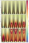 |
Fig. 1. Temperature evolution of the six simulations. From left to right, columns correspond to simulations with σ ∈ {0, 0.75, 1, 1.25, 1.5, 2}. Top row: Snapshots of the simulations at the time at which footpoint driving motion is disabled t = t1. Middle row: Formation of coronal rain (σ = 0), solar prominences (σ = 0 and 0.75), and plasmoids (σ ∈ {1, 1.25, 1.5, 2}). Bottom row: Final snapshot of each simulation. Thin black lines indicate magnetic field lines. The final snapshot occurs at different timestamps for the different σ cases: 253 min (σ ∈ {0, 0.75, 1}), 257 min (σ = 1.25), 234 min (σ = 1.5), and 232 min (σ = 2). An animation of this figure is available https://www.aanda.org/10.1051/0004-6361/202557941/olm. |
The qualitative results, visible in the figure animation, are as follows. At t = t1 (first row), stronger shearing results in a higher location of the flux rope. In addition, stronger shearing heats the flux rope environment more intensely. In all cases, thermal instability forms a solar prominence and coronal rain also forms only for σ = 0. This result is unsurprising, as the σ = 0 case closely resembles our 3D simulated prominence. For σ = 0 and σ = 0.75, the solar prominence escapes the flux rope through mass slippage (Low et al. 2012; Donné & Keppens 2024), but the flux rope does not erupt. In all the other cases, we find prominence eruptions with added diversity: for σ ∈ {1, 1.25}, the solar prominence evaporates during the onset of eruption, whereas for σ ∈ {1.5, 2}, the prominence remains stably in the flux rope throughout CME evolution.
The last row shows the diversity of our results. Two cases (σ = 0 and σ = 0.75) do not erupt, whereas the other four cases do. Two of the four erupting cases do not contain a prominence (σ ∈ {1, 1.25}), while the others do (σ ∈ {1.5, 2}), in agreement with the finding of Low (2001). They argued that, despite an optimal magnetic topology, flux ropes do not always contain a solar prominence because their thermodynamic interiors can vary. Furthermore, in all erupting cases we also obtain plasmoids. We therefore discuss the CME dynamics and energies, the varying thermodynamics of their flux rope interiors, and the synthetic CME morphologies and their agreement with observations. For all data shown, only the results for which the flux rope center satisfies yfrc ≤ 200 Mm are used, unless otherwise specified.
3.1. CME dynamics
By tracking the location of the flux rope center, which is defined as the point of zero magnetic curvature within the flux rope, we obtain a height-time graph. The first panel of Fig. 2 shows this evolution. Flux rope center tracking begins at tfr ≈ 74 min for all cases, and the height is plotted as a function of Δ t = t − tfr. The black line indicates the time at which footpoint motion is disabled. A clear ordering is observed: higher-sheared flux ropes are strictly located at greater heights at each time t, except for σ = 1.25, which is overtaken by σ = 1. The case σ = 0 did not erupt or show any signs of eruption and therefore maintains the same altitude. The σ = 0.75 case did not erupt within the simulation time, but its flux rope center has increased from 16 Mm when the footpoint motion was disabled to 20 Mm at the end of the simulation. The other cases erupted during the simulation time and display an increasing curve, as expected. For the erupting cases σ ∈ {1, 1.25, 1.5, 2}, the flux rope increases in height very slowly, corresponding to the slow-rise phase of the CME. After some time, the flux rope accelerates impulsively. This impulsive phase corresponds to the onset of higher magnetic reconnection rates (Priest 1986; Shibata & Tanuma 2001; Zhao et al. 2017).
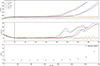 |
Fig. 2. Flux rope evolution for the six shearing cases. Top panel: Height y of the flux rope centers in units of solar radius. Middle panel: Vertical velocity vy in km/s. The time axis is defined as Δ t = t − tfr, where Δ t represents the time elapsed since the flux rope formation. The vertical black line marks the time at which footpoint driving motion is disabled (t = t1 or Δ t = t1 − tfr). Bottom panel: Height evolution of an observed erupting prominence, using data from Di Lorenzo et al. (2025). The final data point of all curves corresponds to the moment when the flux rope center crosses the altitude y = 200 Mm. |
Recently, Liu et al. (2025) and Xing et al. (2024a) demonstrated that the slow-rise phase of the overlying strapping field results from continuous shearing of the magnetic field from footpoint driving motions. Because we disabled footpoint driving motions after flux rope formation, we do not expect expansion of the overlying arcades according to their findings. To compare our results with theirs, we determined the location of the apexes of the magnetic arcades and their associated vertical velocities as follows. Each magnetic field line was computed by following its seedpoint, which co-moves with the local velocity field. When the magnetic field lines are traced from their seedpoints, their apexes are easily obtained by locating the global maximum of the magnetic field lines. We obtained the corresponding vertical velocities of the apexes from the local values of the velocity field at the apex locations. Fig. 3 shows the height evolution (top panel) of the apexes of the central arcades for the σ = 1 simulation, with the corresponding vertical velocities shown in the bottom panel. The other erupting simulations (σ ∈ {1.25, 1.5, 2}) display the same behavior, without significant expansion of the strapping arcades. Vertical velocities of all arcades in all σ cases display values vy < 10 km s−1. Our results are therefore consistent with the interpretation of Xing et al. (2024a) and Liu et al. (2025), indicating that without continuous footpoint driving, the overlying arcades do not undergo significant expansion.
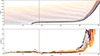 |
Fig. 3. Height y in megameters (top panel) and vertical velocity vy in kilometers per second (bottom panel) of the central arcades’ apexes in function of time t in minutes for σ = 1. Colors ranging from black to orange correspond to lower-lying arcades to higher-lying arcades, respectively. The thick black line corresponds to the evolution of the flux rope center. The vertical red line marks the time at which footpoint driving is disabled (t = t1). |
We focused on explaining the slow-rise phase of the filament. We find that this phase is caused by the slow expansion of the flux rope, which is modulated by magnetic reconnection. To demonstrate this, we characterize the flux rope’s edge by the separatrix, i.e., the line that separates closed magnetic field lines from magnetic arcades. We tracked the separatrix by first searching for points with zero magnetic curvature, following the method of Brughmans et al. (2022). We then used this point as a seedpoint1 for tracing the separatrix along the local magnetic field. Because we defined the flux rope center as the only point with vanishing magnetic curvature within the flux rope, its location is influenced by the size of the flux rope. To illustrate this, Fig. 4 illustrates the expansion of the flux rope during the slow-rise phase for σ = 1, complemented with a schematic cartoon to highlight the ongoing process. The other erupting cases display similar behavior. When magnetic arcades reconnect, they add another magnetic isosurface to the flux rope, resulting in the continual expansion and rise of the flux rope. Fig. 5 further supports this explanation through quantitative analysis. It shows the evolution of the flux rope center height yfrc (top panel), the flux rope’s vertical length Δ yfr (middle panel) and the inflow Alfvén Mach number MA = vx/vA. We calculated the vertical length of the flux rope as the difference between the separatrix’s maximum and minimum height, the latter being the X-point. We computed the inflow Alfvén Mach number MA by taking a 1D horizontal cut of 2 Mm that intersects the X-point, extending 1 Mm to the left and right. We obtained a proxy for the magnetic reconnection rate for by identifying the maximum2 value of MA along this ray.
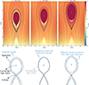 |
Fig. 4. Demonstration of how magnetic reconnection expands the flux rope and shifts its center. Top row: Temperature evolution in megakelvin (MK) for σ = 1. Thin black lines trace magnetic arcades, the thick black line marks the separatrix, and the blue line marks a tracked magnetic arcade that eventually reconnects into a closed magnetic field line. The top white cross marks the flux rope center, defined as the only point within the flux rope with a vanishing magnetic curvature. The lower white cross marks the X-point, defined as another isolated point with zero magnetic curvature. Bottom row: Schematic cartoon illustrating the ongoing process from our simulation in a simplified manner. |
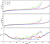 |
Fig. 5. Evolution of flux rope center and vertical dimension for erupting cases σ ∈ {1, 1.25, 1.5, 2} due to magnetic reconnection. Top panel: Height evolution of the flux rope center, yfrc. Middle panel: Vertical length of the flux rope, Δ yfr. Bottom panel: Inflow Alfvén Mach number, MA. The time axis is expressed as Δ t = t − tfr, relative to the onset of flux rope formation, tfr. All curves in the current figure terminate before the formation of their first plasmoids. |
The figure shows that magnetic reconnection is the main driver of the height evolution and expansion of the flux rope. Between Δ t ∈ [0, 30], magnetic reconnection decreases by an order of magnitude, from MA ≈ 2 ⋅ 10−2 to MA ∼ 10−3, as shown in the third panel. Within the same time period, both the flux rope center and vertical length decelerate strongly and accordingly for all erupting σ-cases, as indicated by the top and middle panels, respectively. When magnetic reconnection remains low but non-zero (MA ∼ 10−3), the flux rope expands and rises slowly and steadily for all shown cases in the same time span. The flux rope evolves more rapidly only when the local Mach number increases by an order of magnitude, from MA ∼ 10−3 to MA ∼ 10−2, causing both the flux rope center and the vertical length to increase accordingly with the Mach number. These results further demonstrate a smooth transition from the slow-rise phase to the impulsive phase, which is due to the smooth transition from low Mach number MA ∼ 10−3 to higher Mach number MA ∼ 10−2. In conclusion, our results show that magnetic reconnection dominates the flux rope dynamics in our CMEs, spanning the slow-rise phase to the impulsive phase. These results are consistent with Fan (2017), Xing et al. (2024b), who owed their slow rise to magnetic reconnection as well.
The height-time plot for σ = 1.5 in Fig. 2 shows a clear bump at Δ t ≈ 119 min. This feature is even more evident in the vertical-velocity-time plot in the middle panel of the same figure. We applied a Gaussian smoothing kernel to the velocity curve to smooth out small local gradients. For the other erupting cases (σ ∈ {1, 1.25, 2}), a velocity plateau occurs instead of a bump, at t = 149 min, t = 147 min, and t = 123 min, respectively. The bump and velocity plateaus originate from the first plasmoid formation during the impulsive phase of the CME (see the second row of Fig. 1). Relatively large plasmoids can impede magnetic reconnection (Shibata & Tanuma 2001), slowing the CME’s acceleration in our simulations. As the CME evolves, the effects of subsequent plasmoids are less pronounced. Nevertheless, for all erupting cases, the vertical speed vy reaches ∼40 − 80 km s−1, consistent with observations of erupting prominences (Gopalswamy et al. 2003). The vertical velocity reaches its maximum at Δ t ≈ 147 min for σ ∈ {1.5, 2} and Δ t ≈ 171 min for σ = 1, before decreasing slightly. This behavior indicates that the top boundary at y = 300 Mm affects the CME evolution, limiting further acceleration.
The flux rope centers for σ = 0 and σ = 0.75 exhibit oscillatory behavior, with the oscillation for σ = 0.75 damping over time. Fig. 6 elaborates this mechanism for σ = 0.75, and the same explanation applies to σ = 0. Initially, the flux rope possesses a solar prominence (top-left panel) which subsequently escapes the magnetic flux rope (top-right panel). When the condensation reaches our lower boundary (where we extrapolate assuming constant 1 MK conditions), it gradually evaporates and substantial amounts of pressure enter the simulation box through the bottom boundary, which sustains this high-pressure state. This inflow of high gas pressure pushes on the flux rope and brings it out of its equilibrium position (bottom-right panel). This oscillation thus arises from the 1 MK bottom boundary condition. Thermal conduction primarily drives evaporation at the bottom boundary, as the isothermal T = 1 MK boundary allows the condensation to heat gradually. Although Johnston et al. (2025) show that filaments can escape their magnetic topology by driving the underlying magnetic reconnection, in our simulations the filament likely escapes due to mass slippage, which is consistent with other works that assume almost the same magnetic topology (Jenkins & Keppens 2021, 2022; Donné & Keppens 2024). However, the filament cannot overcome the overlying strapping field and is pushed downward, creating this oscillatory behavior. The oscillation of the σ = 0.75 flux rope dampens over time due to the gradual reduction of pressure effects from the bottom boundary, whereas the σ = 0 boundary maintains energy inflow, which drives the oscillation of the flux rope.
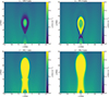 |
Fig. 6. Pressure (p) color plots in centimeter-gram-second units at four timestamps for the σ = 0.75 case. |
Overall, our dynamical results are in good agreement with observations of erupting prominences. An observed erupting prominence, courtesy of Di Lorenzo et al. (2025), is shown in the bottom panel of the same figure. From Δ t ≈ 1094 min onward, the prominence exhibits a conspicuously non-linear height-time profile, suggesting that the slow-rise phase of this observed case lasts for ≈1094 min. Although our idealized 2.5D configuration (with a flux rope disconnected from the surface) and lack of fine-tuning produce a prominence eruption timescale of τ ∼ 180 min, which is much shorter than this specific observation, the overall trend remains similar. Extending this work to a more realistic 3D model would be useful, as line-tying effects will delay eruptions and allow prominence drainage along the flux rope axis (see Fan 2017, 2018).
3.1.1. Energetics of the CMEs
We further interpreted the height-time plot by computing the magnetic free-energy eMFR, kinetic- ekin, and thermal energy densities ethe within the entire simulation box (i.e., |x|≤30 Mm and |y|≤300 Mm). We also calculated the average energy density seepage eseep, which quantifies how much energy has already flowed out of our domain. We computed the magnetic free energy by first constructing the potential field following Chiu & Hilton (1976), Xia et al. (2018) and subsequently subtracting the total magnetic energy from the potential energy. The average energy density seepage considers all flux terms in the energy equation, i.e., compressional heating, Poynting flux, thermal conduction, Ohmic heating, background heating, radiative cooling, and gravitational work. These flux contributions were summed into a net flux and subsequently integrated over the entire simulation domain to obtain the average energy seepage rate. To express the seepage in units of energy density, we divided the average energy seepage rate by the simulation volume and integrated it with time. This yields the average energy density seepage eseep which is a cumulative quantity. In mathematical form, eseep is expressed as
 (8)
(8)
where 𝒱 denotes the simulation domain, (∇⋅F)|net represents the net flux of all conservative terms, and Snet is the net flux of all the source and sink terms. In this definition, eseep(t)> 0, indicates energy seeping into the domain, whereas eseep(t)< 0 specifies energy leaking out. We numerically evaluated the time integral in eseep by integrating over the uniform times between the output files rather than the Courant–Friedrichs–Lewy (CFL) time step of the simulation. Hence, the cumulative energy seepage density is a rough estimate. Fig. 7 presents these results alongside the height-time plot from Fig. 2. The flux rope forms at t ≈ 73 min, which is when the tracking began. For t ≲ 73 min, the flux rope is absent, so we set its center at the bottom of our simulation domain (y = 0 or y = 1 R⊙).
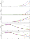 |
Fig. 7. Height evolution (top panel), average kinetic energy density (second panel), average thermal energy density (third panel), average magnetic free energy density (fourth panel), and average seeped energy density (last panel) for the six different σ-cases. The vertical black line marks the time at which footpoint motion is off (t = t1). Energy densities are expressed in erg cm−3 and are averaged over the entire simulation domain |x|< 30 Mm and y < 300 Mm. |
The second panel shows the kinetic energy density of the simulation. For erupting cases (σ ∈ {1, 1.25, 1.5, 2}), the kinetic energy density becomes significant once the CME is going through its impulsive phase and reaches energies on the order of ekin ∼ 10−3 erg cm−3. The gray curve (σ = 0) shows fluctuations during 98 min ≲ t ≲ 167 min. These arise from coronal rain, which has a similar density to the solar prominence but reach significant speeds up to |v|∼60 km s−1. Coronal rains form at t ≈ 98 min and fall to the bottom part of our simulation domain at t ≈ 167 min. The beige curve (σ = 0.75) shows negligible kinetic energy.
The erupting case in which the prominence evaporates (σ = 1) has a higher final kinetic energy density than the other erupting cases where the prominence remains (σ ∈ {1.5, 2}). Although the total kinetic energy density is computed over the entire simulation domain, the erupting flux rope is the dominant component. This higher kinetic energy arises because the erupting, evaporated prominences have higher peak speeds (80 − 85 km s−1) than the erupting, non-evaporated prominences (≈65 km s−1), as seen in Fig. 2. However, the final kinetic energy of σ = 1.25 is lower than that of σ = 1, because the prominence in the σ = 1 case evaporates before the prominence in σ = 1.25, which can also be seen in the animation of Fig. 1. These results indicate that the prominence inhibits the flux rope from attaining fast acceleration. These results agree with Zhao et al. (2017), who demonstrate that the solar prominence dominates the evolution of the flux rope.
The third panel displays the thermal energy density. During footpoint driving (before the vertical black line) σ-cases show minor variation. However, after flux rope formation, the curves diverge significantly from each other. The gray curve (σ = 0) is the only one that reaches a thermal energy density below the initial thermal value (ethe, 0) between 98 min ≲ t ≲ 167 min, which is due to the formation of coronal rain. After 167 min ≲ t, the thermal energy density increases, although there is no significant magnetic reconnection. This increase arises partly from the pressure-driven effects discussed in Fig. 6 for σ = 0.75 and partly from our open side boundaries3 after t1 < t. Consequently, the thermal energies increase in both cases. The thermal energy density of the gray curve flattens, whereas the beige curve (σ = 0.75) continues to increase steadily. This difference reflects the ongoing magnetic reconnection for σ = 0.75, which drives its thermal energy increase similarly to that of the erupting cases (σ ∈ {1, 1.25, 1.5, 2}). In these five σ-cases, the magnetic free energy density (fourth panel) continuously decreases, converting its kinetic and thermal energy density, which is not the case for σ = 0. The σ = 0 flux rope undergoes mass depletion but does not erupt, possibly because it reaches a height where mass depletion does not bring it out of equilibrium, as shown by Jenkins et al. (2019). They argue that a critical height exists above which mass depletion can cause the flux rope to erupt. Since our case of σ = 0 does not erupt, it is clear that it has not reached this critical height. In Fan (2018), prominence draining facilitated the onset of the kink instability. In addition, prominence draining can also aid in the onset of torus instability by reducing the stabilizing effect of gravity, as demonstrated in recent 3D simulations by Xing et al. (2025). More studies are needed to extend this work to 3D and examine whether our flux rope undergoes kink or torus instability.
While the kinetic and thermal energy densities only become noticeable after t = t1, the magnetic free energy density eMFE shows clear differences between the σ-cases during footpoint driving t ≤ t1. During the footpoint driving t ≤ t1, higher shearing σ corresponds directly to higher eMFE, indicating a higher energy state of the flux rope, as expected. Once footpoint driving is disabled (t1 < t), all cases except σ = 0 show a steady decrease. Indeed, CME theory requires the magnetic energy to decrease as the flux rope searches for a new equilibrium at higher altitudes. In particular, even the beige curve (σ = 0.75) shows a decreasing magnetic free energy density, despite it not erupting. This suggests that if the simulation time was extended, it would likely erupt eventually. This hypothesis is also motivated by the slight increase in its flux rope center, which climbs from 16 Mm when the footpoint motion is disabled to 20 Mm at the end of its simulation. The gray curve (σ = 0) exhibits a decrease in magnetic free energy density around t ≈ 175 min, but after t ≈ 225 min it remains quasi-stable again. Because the σ = 0 flux rope center does not shows a significant increase in altitude, we believe that it will not erupt unless footpoint shearing continues indefinitely.
The bottom panel shows the cumulative energy density seepage eseep. During footpoint driving (before the vertical black line), energy flows into the domain from the bottom boundary treatment, inducing shearing of the magnetic field lines as expected. After disabling footpoint driving, all cases except σ = 0 exhibit negative seepage values, indicating energy flowing out of our domain.
From these results, we can quantify the conversion rates of magnetic free energy density into thermal and kinetic energy density and examine the efficiency of magnetic flux cancelation in driving a CME. To obtain a consistent result, we define the change in magnetic free energy density Δ eMFE as the difference between the global minimum and maximum of the curve, Δ eMFE ≡ eMFE, min − eMFE, max, where eMFE, max and eMFE, min denote the maximum and minimum attained magnetic free energy densities, respectively. We then use the corresponding timestamps τMFE, max and τMFE, min to determine the instantaneous thermal and kinetic energy densities and to define the corresponding changes in the energy density, Δ ethe and Δ ekin, respectively. We further define the energy conversion percentage ϵ as
 (9)
(9)
which allows us to quantify the conversion rates. Table 1 presents these values. Since our boundaries are partially open, the value of eseep from Fig. 7 indicates that the simulation loses energy, either through sink terms such as radiative cooling or through energy flowing out of the boundaries. Table 1 rates are thus indicative only.
Energy conversion from magnetic to kinetic and thermal energy densities as a function of shearing σ.
From the table, it is clear that increased shearing σ results in a higher obtained maximum magnetic free energy density eMFE, max at earlier times τMFE, max. However, eMFE, max varies only weakly between the different σ cases, with the largest relative difference being 2.1%. It is important to note that this quantity relates to the total energy of the magnetic field. Nevertheless, this small relative difference in total magnetic energy produces diverse phenomena, including eruption versus no eruption, prominence evaporation versus prominence maintenance, and morphological difference, as discussed later. All erupting cases exhibit a systematically larger decrease in magnetic free energy density than the non-erupting cases, suggesting an energetic separation between the erupting and non-erupting regimes.
To compare energy conversions among the different σ-cases, the quantity Δ e/Δ τ is more relevant, as it normalizes the change in energy density by the corresponding time period. In particular, ϵ makes the comparison more simple and convenient, as it is expressed as a percentage. From Table 1, it is immediately apparent that the conversion from magnetic to kinetic energy density is small, reaching at most ≈10% of the magnetic free energy density rate. Instead, a substantial fraction of the magnetic free energy density in the erupting cases is converted into thermal energy density, heating the plasma with values ranging from 29%−57%, while another fraction is lost through energy seeping out of the domain, as shown in Fig. 7. Moreover, our relatively high resistivity results in higher magnetic diffusion. Therefore, the inefficiency of converting magnetic free energy into kinetic energy to push the flux rope could be specific to our simulation setup. Different boundary conditions and resistivity values in our study affect this efficiency: the former limit energy seeping out of the domain, while the latter constrain magnetic energy conversion into heat. Furthermore, increasing σ does not imply a proportionate increase in either kinetic or thermal energy density. This is evident from the values of Δ e/Δτ and ϵ for both kinetic and thermal energy densities, which do not show a monotonic increase. Finally, we note that the magnetic free energy densities obtained here, e ∼ 0.4 erg cm−3, are consistent with energy densities inferred for observed CMEs (Chen 2011).
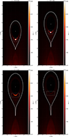 |
Fig. 8. Tracking of the prominence for σ = 1 in the synthetic 304 Å channel. The dashed white rectangle marks the region over which the average is computed in Fig. 9. The x and y coordinates are given in megameters. The solid white line marks the separatrix of the magnetic flux rope. |
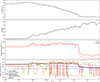 |
Fig. 9. Evolution of the average density in 109 cm−3 (first panel), average temperature in MK (second panel), average synthetic 171 Å and 304 Å intensities in DN s−1 (third panel), and the relevant energy fluxes from the energy equation (fourth panel). All quantities are averaged within a region around the prominence indicated in Fig. 8. In the fourth panel we display the absolute value of radiative cooling. The data include averaged values before, during, and after the evaporation. |
3.2. Varying thermodynamical environments of flux rope interiors
Interestingly, coronal rain occurs only for σ = 0, not for σ > 0. These results suggest that coronal rain formation is promoted only in low energy states (0 ≤ σ < 0.75), likely due to the ambient heating resulting from flux rope formation. As Low (2001) explains, the flux rope interior remains thermally isolated because of long magnetic field lines and the inefficiency of thermal conduction perpendicular to the magnetic field. Within this thermally isolated environment, instabilities related to condensations, such as solar prominences, are likely to occur. In contrast, coronal rain forms outside the flux rope and is not thermally isolated. The reduced dimensionality of our setup also plays a role: our previous 3D simulation (Donné & Keppens 2024) showed evidence of rain forming above the forming flux rope, where pressure-induced thermodynamic changes trigger thermal instability. Future 3D studies with varying σ should examine how different driving conditions influence the likelihood of rain formation during flux rope evolution.
For the higher shearing cases (σ = 1 and σ = 1.25), the prominences evaporate during the eruption initiation. Wang et al. (2016) observed solar prominence evaporation, but could only speculate on the underlying causes, including thermal conduction between the hot corona and cold prominence. Our simulated evaporated prominences confirm that thermal conduction and compressional heating drive prominence evaporation.
To verify that we simulate prominence evaporation, we analyzed σ = 1 within a rectangle around the evaporation, as shown in Fig. 8 which displays the synthetic 304 Å channel of the Atmospheric Imaging Assembly (AIA) onboard the Solar Dynamics Observatory (SDO), as used by Wang et al. (2016). Within this rectangle, we averaged over the number density n, temperature T, the 171 Å and 304 Å synthetic intensities, and all relevant energy fluxes. Fig. 9 shows the results.
The first and second panels show the average number density ⟨n⟩ and temperature ⟨T⟩ and help us to demarcate the stages of evaporation. For t < 176 min, the average density and temperature maintain a quasi-stable value of ⟨n⟩≈2 ⋅ 109 cm−3 and ⟨T⟩≈0.5 MK. Between 176 min ≤ t ≤ 219 min, the density steadily decreases, whereas the temperature increases, consistent with an evaporating fluid. After t ≥ 219 min, all prominence material vanishes, resulting in a typical coronal density of ∼108 cm−3 and a temperature of ∼2 MK. This result demonstrates that our simulations self-consistently retrieve an evaporating prominence. The time t < 176 min marks the pre-evaporation phase, 176 min ≤ t ≤ 219 min is the evaporation phase, and t ≥ 219 min is the post-evaporation phase.
The third panel shows the averaged synthetic intensities. Before prominence evaporation, the averaged synthetic intensities assume their baseline values around 10−7 DN s−1. Between 176 min ≤ t ≤ 219 min, the prominence evaporates and the intensities increase significantly over a duration of ≈43 min. Once the prominence disappears, the intensity decreases by an order of magnitude for 171 Å and nearly two orders of magnitude for 304 Å. This trend is in very good agreement with the intensity evolution reported by Wang et al. (2016). The close agreement between our calculated intensity values with the observed intensities of Wang et al. (2016) provides observational verification of our results.
Having established that our simulation reproduces an evaporating prominence, we next examine the cause of this evaporation. The last panel displays all fluxes from the energy equation, except the gravitational potential energy rate, which is negative in the demarcated region of Fig. 8. We show the absolute value of the radiative cooling rate (identified by the thick black line). Only fluxes that are positive and exceed the absolute radiative cooling rate can heat the prominence until evaporation. Ohmic heating (blue line) and our static background heating (purple line) are much smaller in magnitude than the radiative cooling rate and hence cannot evaporate a prominence. Although the Poynting flux (beige line) occasionally reaches values comparable to radiative cooling, it remains mostly weaker4. Only thermal conduction (red line) consistently dominates over radiative cooling throughout the evaporation phase, at a value of ∼10−2 erg cm−3 s−1. Additionally, compressional heating (green line) is comparable to radiative cooling and sometimes exceeds it in magnitude. After evaporation, thermal conduction decreases, while compressional heating remains high at ∼10−2 erg cm−3 s−1. This value is almost in perfect agreement with Lee et al. (2017), who estimate the heating rate of an erupting prominence at 0.05 − 0.08 erg cm−3 s−1. However, in their article, the erupting prominence did not evaporate. We conclude that thermal conduction and compressional heating are the important drivers in evaporating a solar prominence. These processes may also heat erupting filaments without causing evaporation, potentially explaining the heated erupting filaments observed by Landi et al. (2010) and Lee et al. (2017). Additionally, Sieyra et al. (2026) used data-driven simulations to model an observed CME, showing that compression contributes to both flux rope formation and heating. To our knowledge, this is the first simulation-based study to explicitly demonstrate prominence evaporation driven by thermal conduction and compressional heating during a CME eruption.
To provide a meaningful comparison of the prominence among the four erupting cases, we averaged the density and temperature over the regions T ≤ 0.1 MK and calculated the total prominence mass. Figure 10. presents this comparison. The figure shows that higher energy states, σ, delay the formation of the solar prominence. This agrees with our earlier observation that the temperatures of the flux rope and its ambient environment increase with increasing σ, implying that radiative cooling requires more time to cool down from the hotter flux rope temperatures to the prominence temperature of Tmin ≈ 0.1 MK. For all cases, the average density initially rises rapidly and subsequently increases very slowly. For the blue and red curves (σ ∈ {1, 1.25}), the average density increases substantially after t ≳ 176 min. This increase in average density agrees with our earlier work (Donné & Keppens 2024) (see discussion related to their Fig. 3), where we argue that most of the prominence mass, undergoing minor evaporation, is stored in cold condensations with T ≤ 0.025 MK. In our current simulations, since these denser condensations reside deeply within the prominence, shielded by less dense condensations (0.025 MK < T ≤ 0.1 MK), the less dense condensations evaporate first, leaving the more dense condensations (T < 0.025 MK) behind, which causes the average density n to increase for both curves. This is confirmed by the average temperature in the second panel, which shows that during evaporation for 176 min ≤ t and 190 min ≤ t for σ = 1 and σ = 1.25, respectively, the average temperature remains close to T ∼ 0.025 MK. Only when thermal conduction and compressional heating reach the denser condensations does the average temperature rise sharply at t ≈ 219 min for σ = 1. For the purple (σ = 1.5) and green (σ = 2) curves, the average density decreases after roughly 185 min < t, which marks the instant when the flux rope erupts for both cases (Fig. 2). Despite the decreasing density, the mass steadily increases for both curves, shown in the bottom panel. The total mass of the red and blue curves reduces to zero as a result of complete evaporation and disappearance of the prominence.
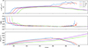 |
Fig. 10. Average density n in cubic centimeters (top panel), average temperature T in megakelvin (middle panel), and total prominence mass M in grams per centimeter (bottom panel) for the erupting case σ ∈ {1, 1.25, 1.5, 2}. The prominence is defined as regions where T ≤ 0.1 MK. |
3.3. Observational similarities
After established the key novelties in our parametric study of filament-CME eruptions and confirming quantitative agreements with observations, we now correlate our findings with direct satellite observations and highlight morphological similarities. We used the AIA Filament Eruption Catalog5 (McCauley et al. 2015) to identify early evolutions of filament eruptions observed by the SDO/AIA instrument (Lemen et al. 2012).
Fig. 11 shows a filament eruption observed on 07 October 2010 located at the NW limb and seen through the 171 Å channel. The eruption exhibits a bright fan that eventually disappears, giving rise to a conspicuous cusp structure and post-eruptive arcades, features commonly observed following CME events (Tripathi et al. 2004). Our synthetic results in the same channel for σ = 1 reproduce this evolution, showing a similar fan structure that also disappears over time. Our results show that this fan structure corresponds to the current sheet, where the density is n ∼ 3 ⋅ 108 cm−3 and the temperature is T ∼ 2 MK. When the fan disappears, the density remains roughly constant, whereas the temperature reaches values up to T ∼ 4 MK. This increase results in an order-of-magnitude decrease in intensity compared to temperatures at T ∼ 2 MK due to the sensitivity of the temperature response function of 171 Å. Following the eruption and disappearance of the fan, a dark cusp-shaped region forms, which then gives way to post-eruptive arcades. In our simulation, the cusp-shaped region also appears and forms simultaneously with the post-eruptive arcades, which have temperatures around T ∼ 1.3 MK.
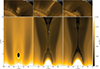 |
Fig. 11. Top row: Observed filament eruption evolution in the 171 Å channel. First panel: Filament before eruption. Second panel: Bright fan after eruption (arrow and dashed line), which eventually disappears. Third panel: Post-eruptive arcades (white arrow). Bottom row: Simulated σ = 1 results in the synthetic 171 Å channel at instrument resolution, highlighting the same structures with white arrows and dashed lines. Observational images are retrieved from the AIA Filament Eruption Catalogue. |
Fig. 12 compares two observations of erupting prominences exhibiting strong circular patterns, viewed from different satellites, alongside our complementing synthetic images. The top-left panel shows a white-light image taken by the COR2 coronagraph onboard the Solar Terrestrial Relations Observatory Ahead (STEREO-A), showing the CME with a semi-bright core surrounded by a small dark gap, a bright ring, another gap, and a smaller bright ring. Because white-light intensity depends on the local electron density (Howard & Tappin 2009), these bright rings can indicate regions of higher local electron density, while the gaps indicate lower-density regions. The top-right panel shows a separate event observed by SDO/AIA in the 304 Å channel, where the circular pattern is more pronounced. This demonstrates that fine structures, such as the circular pattern, can be detected in the low corona. The bottom-left and bottom-right panels show synthetic images in the 304 Å and 193 Å channels for the σ = 2 case. These synthetic images successfully reproduce the observed circular pattern.
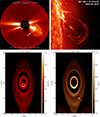 |
Fig. 12. Top row: Separate observed events through different satellites. Top-left: White-light image from STEREO-A Cor2 of an erupting filament, displaying a clear circular pattern. Top-right: Different event as observed with SDO/AIA in the 304 Å channel, also showing a clear circular pattern. Bottom row: Synthetic images for the σ = 2 case at instrument resolution. Bottom-left: 304 Å channel. Bottom-right: 193 Å channel. Blue and white arrows indicate dark structures, also marked by dashed lines of the same color, which correspond to features analyzed in Fig. 13. Observational images are from the AIA Filament Eruption Catalog. |
Fig. 13 presents our analysis of circular pattern origins. The three panels display the evolution along the central vertical axis x = 0 for the density, temperature, and intensity of the synthesized 193 Å channel, all measured in the reference frame of the flux rope center. Here, Δ y = 0 corresponds to the flux rope center. Within the flux rope, several dark and bright regions are clearly visible in the synthetic emission. Comparing the density and temperature evolution with the synthetic intensity, we find that the darker rings or gaps arise from extreme temperatures: either T < 0.1 MK in the prominence or T > 2.5 MK, where the density is roughly n ∼ 0.25 × 109 cm−3.
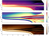 |
Fig. 13. Evolution of the density in 109 cm−3 (top panel), temperature in MK (middle panel), and intensity in the synthetic 193 Å channel (bottom panel) along the central vertical axis x = 0 in the reference frame of the flux rope center. The height with respect to the flux rope center is denoted by Δ y, and the time relative to the moment when the flux rope center is tracked is denoted by Δ t. |
In contrast, the bright regions have roughly double the flux rope average density (n ∼ 0.5 × 109 cm−3) and temperatures around T ∼ 1.5 MK. The bright circular pattern is therefore a combination of enhanced density and suitable temperature, since the temperature response function of the 193 Å channel peaks at 106.2 K ≈ 1.6 MK. Consequently, the darker rings can be either hot, cold, sparse, or dense.
Interestingly, plasmoids can also produce dark rings in the synthetic image. At times, plasmoids interact with the flux rope, producing a local darkening in the synthetic intensity after a short delay and creating a dark gap. Although the density in this gap can be relatively high (n ∼ 0.6 × 109 cm−3), the temperature exceeds 2 MK, where the temperature response function is significantly reduced. We also note the presence of additional dark structures that recede from the flux rope center. These features correspond to the interaction interface between the erupting flux rope and the plasmoids generated in the current sheet.
Although plasmoids can contribute to darker gaps in the synthetic images, they are not sufficient alone. Fig. 14 illustrates the different morphologies of the erupting flux ropes for the various erupting cases σ. All erupting cases (σ ∈ {1, 1.25, 1.5, 2}) form plasmoids, but only σ = 2 shows a very strong annular pattern in the synthetic image. The σ = 1.25 case shows a small dark ring, less pronounced than σ = 2. This suggests that the morphology of erupting flux ropes is highly sensitive to the energy state of the flux rope, although the largest relative difference in maximum magnetic energy between the cases σ is only 2.1%.
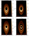 |
Fig. 14. Morphology of the erupting flux ropes in the synthetic 193 Å channel for σ = 1 (top-left), σ = 1.25 (top-right), σ = 1.5 (bottom-left), and σ = 2 (bottom-right). |
4. Summary and conclusion
We have examined the response of the flux rope to slight variations in its energy state, i.e., increased shearing during flux rope formation. The largest relative difference between the maximal magnetic energy achieved among the different shearing cases σ is only 2.1%. Despite this low value, our erupting prominences produce a rich variety of phenomena.
For σ = 0, the flux rope does not show an eruption, while for σ = 0.75, the flux rope center increases slightly in altitude. Given its continuously decreasing magnetic energy, we speculate that it will eventually erupt if we extend our simulation time. The cases σ ∈ {1, 1.25, 1.5, 2} all erupt. From the quantifications in Table 1, flux ropes with higher energy states erupt more rapidly. However, higher energy states σ do not correspond directly to proportionally higher conversion rates to kinetic and thermal energy. Furthermore, the erupting cases display a slow-rise phase of the CME. Liu et al. (2025) attribute this slow-rise phase to the expansion of the overlying arcade field, but our results show that this is not a necessary condition, as our overlying arcades do not expand noticeably. Magnetic reconnection itself can reproduce the slow-rise phase, in agreement with Fan (2017), Xing et al. (2024b). We note that our 2.5D setup captures only the central dynamics of a full 3D erupting flux rope. For instance, 2.5D simulations cannot capture prominence draining along field lines, which in fully 3D configurations can contribute to or even drive the slow-rise phase, as suggested by Fan (2020) and demonstrated by Xing et al. (2025). In this context, we demonstrate that prominence eruption in our simulation is governed by magnetic reconnection, as indicated by the inflow Alfvén Mach number increasing by an order of magnitude compared to the slow-rise phase.
Comparing the thermodynamics of the solar prominences, we find that for σ ∈ {1, 1.25}, the prominence evaporates. This evaporation is due to thermal conduction and compressional heating. Our quantification of the average synthetic intensities in the 304 Å and 171 Å channels during prominence evaporation shows excellent agreement with observations (Wang et al. 2016). This unique finding, which has never been demonstrated before in the literature, demonstrates that thermal conduction and compressional heating are critical not only for evaporating solar prominences but also for heating the flux rope interior. For σ = {1.5, 2}, the prominence remains present throughout the eruption. These results verify that flux rope interiors are unique and susceptible to strongly varying thermodynamics, consistent with Low (2001). Extending our simulations of σ ∈ {1, 1.25} to 3D would allow us to examine whether prominence evaporation still persists under fully 3D conditions. If evaporation persists under 3D conditions and it would indeed endure these dominant fluxes, our idealized setup could be a strong model candidate for the event observed by Lee et al. (2017), given that the heating rates of our erupting prominences already agree closely in 2.5D with their observed filament eruptions. This would further support our argument for the clear thermodynamic role of thermal conduction and compressional heating in prominence eruptions.
We conclude by drawing parallels with observations. Our simulations reproduce a fan structure following prominence eruption. Additionally, for the first time as well, we retrieve fine structures such as circular patterns in our synthetic extreme ultraviolet (EUV) data for σ = 2, which correspond to features observed in white-light images (Dere et al. 1999; Vourlidas et al. 2013). The bright rings result from high density relative to other regions in the flux rope and temperatures that align with the peak values of SDO/AIA temperature response functions. The darker gaps or rings in this circular pattern can indicate hot, cold, dense, and/or sparse regions. We also show for the first time that plasmoids can contribute to the CME fine structure by causing a dark ring in this circular pattern. However, plasmoid formation alone is not sufficient as other σ-cases also generate plasmoids but do not always possess a noticeable circular pattern in their synthetic images. These results suggest that fine structures observed in the white light in the heliosphere can pre-exist in the low corona. More research is needed to validate this hypothesis by extending the physical domain up to heliospheric scales to determine whether these fine structures persist throughout CME evolution.
In future work, our aim is to implement a 3D model of our prominence eruptions. Using spherical coordinates and extending the top boundary to 10 solar radii will enable synthetic white-light images and facilitate comparisons with observations. While 2.5D simulations are constrained to a plane-of-the-sky view, 3D simulations will reveal CME morphology through different angles and allow investigation of projection effects.
Data availability
Movie associated with Fig. 1 is available at https://www.aanda.org
Acknowledgments
The authors want to thank the anonymous referee for the valuable feedback which has improved the quality of this article. DD and HC acknowledge that the research was sponsored by the DynaSun project and has thus received funding under the Horizon Europe programme of the European Union under grant agreement (no. 101131534). Views and opinions expressed are however those of the author(s) only and do not necessarily reflect those of the European Union and therefore the European Union cannot be held responsible for them. The computational resources and services used in this work were provided by the VSC (Flemish Supercomputer Center), funded by the Research Foundation Flanders (FWO) and the Flemish Government, department EWI. RK acknowledges funding from the KU Leuven C1 project C16/24/010 UnderRadioSun and the Research Foundation Flanders FWO project G0B9923N Helioskill. YZ acknowledges the support from the Jiangsu Provincial Double First-Class Initiative (grant number 1480604106).
References
- Amari, T., Luciani, J. F., Mikic, Z., & Linker, J. 2000, ApJ, 529, L49 [NASA ADS] [CrossRef] [Google Scholar]
- Antiochos, S. K., DeVore, C. R., & Klimchuk, J. A. 1999, ApJ, 510, 485 [Google Scholar]
- Berger, T. E., Slater, G., Hurlburt, N., et al. 2010, ApJ, 716, 1288 [Google Scholar]
- Brughmans, N., Jenkins, J., & Keppens, R. 2022, A&A, 668, A47 [NASA ADS] [CrossRef] [EDP Sciences] [Google Scholar]
- Chen, P. F. 2011, Liv. Rev. Sol. Phys., 8, 1 [Google Scholar]
- Chiu, Y. T., & Hilton, H. H. 1976, BAAS, 8, 370 [Google Scholar]
- Cremades, H., & Bothmer, V. 2004, A&A, 422, 307 [NASA ADS] [CrossRef] [EDP Sciences] [Google Scholar]
- Cremades, H., Bothmer, V., & Tripathi, D. 2006, Adv. Space Res., 38, 461 [NASA ADS] [CrossRef] [Google Scholar]
- Del Moro, D., Giordano, S., & Berrilli, F. 2007, A&A, 472, 599 [NASA ADS] [CrossRef] [EDP Sciences] [Google Scholar]
- Dere, K. P., Brueckner, G. E., Howard, R. A., Michels, D. J., & Delaboudiniere, J. P. 1999, ApJ, 516, 465 [NASA ADS] [CrossRef] [Google Scholar]
- Di Lorenzo, L., Cremades, H., López, F., et al. 2025, Sol. Phys., submitted [Google Scholar]
- Donné, D., & Keppens, R. 2024, ApJ, 971, 90 [CrossRef] [Google Scholar]
- Dorman, L. I., Ptitsyna, N. G., Villoresi, G., et al. 2008, Adv. Geosci., 14, 271 [Google Scholar]
- Fan, Y. 2017, ApJ, 844, 26 [Google Scholar]
- Fan, Y. 2018, ApJ, 862, 54 [Google Scholar]
- Fan, Y. 2020, ApJ, 898, 34 [Google Scholar]
- Field, G. B. 1965, ApJ, 142, 531 [Google Scholar]
- Filippov, B., & Koutchmy, S. 2002, Sol. Phys., 208, 283 [Google Scholar]
- Forbes, T. G. 2000, J. Geophys. Res., 105, 23153 [Google Scholar]
- Georgoulis, M. K., Nindos, A., & Zhang, H. 2019, Philos. Trans. Roy. Soc. London Ser. A, 377, 20180094 [Google Scholar]
- Gibson, S. E., & Low, B. C. 1998, ApJ, 493, 460 [NASA ADS] [CrossRef] [Google Scholar]
- Glesener, L., Krucker, S., Bain, H. M., & Lin, R. P. 2013, ApJ, 779, L29 [NASA ADS] [CrossRef] [Google Scholar]
- Gopalswamy, N., Shimojo, M., Lu, W., et al. 2003, ApJ, 586, 562 [NASA ADS] [CrossRef] [Google Scholar]
- Green, L. M., Török, T., Vršnak, B., Manchester, W., & Veronig, A. 2018, Space Sci. Rev., 214, 46 [Google Scholar]
- Howard, T. A., & Tappin, S. J. 2009, Space Sci. Rev., 147, 31 [NASA ADS] [CrossRef] [Google Scholar]
- Illing, R. M. E., & Hundhausen, A. J. 1985, J. Geophys. Res., 90, 275 [Google Scholar]
- Jenkins, J., & Keppens, R. 2021, A&A, 646, A134 [NASA ADS] [CrossRef] [EDP Sciences] [Google Scholar]
- Jenkins, J. M., & Keppens, R. 2022, Nat. Astron., 6, 942 [NASA ADS] [CrossRef] [Google Scholar]
- Jenkins, J. M., Hopwood, M., Démoulin, P., et al. 2019, ApJ, 873, 49 [Google Scholar]
- Johnston, C. D., Daldorff, L. K. S., Schuck, P. W., et al. 2025, ApJ, 982, 131 [Google Scholar]
- Kaneko, T., & Yokoyama, T. 2017, ApJ, 845, 12 [Google Scholar]
- Kaneko, T., & Yokoyama, T. 2018, ApJ, 869, 136 [Google Scholar]
- Keppens, R., Popescu Braileanu, B., Zhou, Y., et al. 2023, A&A, 673, A66 [NASA ADS] [CrossRef] [EDP Sciences] [Google Scholar]
- Keppens, R., Zhou, Y., & Xia, C. 2025, Liv. Rev. Solar Phys., 22, 4 [Google Scholar]
- Landi, E., Raymond, J. C., Miralles, M. P., & Hara, H. 2010, ApJ, 711, 75 [Google Scholar]
- Lee, J.-Y., Raymond, J. C., Reeves, K. K., Moon, Y.-J., & Kim, K.-S. 2017, ApJ, 844, 3 [NASA ADS] [Google Scholar]
- Lemen, J. R., Title, A. M., Akin, D. J., et al. 2012, Sol. Phys., 275, 17 [Google Scholar]
- Li, X., Zhou, Y., & Keppens, R. 2025, A&A, 698, A232 [NASA ADS] [CrossRef] [EDP Sciences] [Google Scholar]
- Liu, Q., Jiang, C., & Liu, Z. 2025, RAA, 25, 051002 [Google Scholar]
- Low, B. C. 2001, J. Geophys. Res., 106, 25141 [NASA ADS] [CrossRef] [Google Scholar]
- Low, B., Liu, W., Berger, T., & Casini, R. 2012, ApJ, 757, 21 [Google Scholar]
- McCauley, P. I., Su, Y. N., Schanche, N., et al. 2015, Sol. Phys., 290, 1703 [NASA ADS] [CrossRef] [Google Scholar]
- Parker, E. N. 1953, ApJ, 117, 431 [Google Scholar]
- Priest, E. R. 1986, Mitteilungen der Astronomischen Gesellschaft Hamburg, 65, 41 [Google Scholar]
- Sen, S., Nayak, S. S., & Antolin, P. 2025, A&A, 703, A241 [NASA ADS] [CrossRef] [EDP Sciences] [Google Scholar]
- Shibata, K., & Tanuma, S. 2001, Earth Planets Space, 53, 473 [NASA ADS] [CrossRef] [Google Scholar]
- Sieyra, M. V., Strugarek, A., Prasad, A., et al. 2026, A&A, submitted [Google Scholar]
- Terradas, J., Soler, R., Luna, M., Oliver, R., & Ballester, J. 2015, ApJ, 799, 94 [Google Scholar]
- Tripathi, D., Bothmer, V., & Cremades, H. 2004, A&A, 422, 337 [NASA ADS] [CrossRef] [EDP Sciences] [Google Scholar]
- Tsurutani, B., & Lakhina, G. S. 2019, AGU Fall Meeting Abstracts, 2019, SM13E–3352 [Google Scholar]
- Vourlidas, A. 2014, Plasma Phys. Control. Fusion, 56, 064001 [CrossRef] [Google Scholar]
- Vourlidas, A., Lynch, B. J., Howard, R. A., & Li, Y. 2013, Sol. Phys., 284, 179 [NASA ADS] [Google Scholar]
- Wang, B., Chen, Y., Fu, J., et al. 2016, ApJ, 827, L33 [NASA ADS] [CrossRef] [Google Scholar]
- Webb, D. F., & Howard, T. A. 2012, Liv. Rev. Sol. Phys., 9, 3 [Google Scholar]
- Xia, C., & Keppens, R. 2016, ApJ, 825, L29 [NASA ADS] [CrossRef] [Google Scholar]
- Xia, C., Teunissen, J., El Mellah, I., Chané, E., & Keppens, R. 2018, ApJS, 234, 30 [Google Scholar]
- Xing, Y., Duan, A., & Jiang, C. 2024a, MNRAS, 534, 107 [Google Scholar]
- Xing, C., Aulanier, G., Cheng, X., Xia, C., & Ding, M. 2024b, ApJ, 966, 70 [Google Scholar]
- Xing, C., Cheng, X., Aulanier, G., & Ding, M. 2025, ApJ, 986, 37 [Google Scholar]
- Yoshihisa, T., Yokoyama, T., & Kaneko, T. 2025, ApJ, 978, 94 [Google Scholar]
- Zaitsev, V. V., & Stepanov, A. V. 2018, J. Atmos. Sol. Terr. Phys., 179, 149 [Google Scholar]
- Zhao, X., & Keppens, R. 2022, ApJ, 928, 45 [NASA ADS] [CrossRef] [Google Scholar]
- Zhao, X., Xia, C., Keppens, R., & Gan, W. 2017, ApJ, 841, 106 [Google Scholar]
- Zhou, Y.-H., Chen, P.-F., Zhang, Q.-M., & Fang, C. 2014, RAA, 14, 581 [Google Scholar]
- Zhou, Y., Li, X., Hong, J., & Keppens, R. 2023, A&A, 675, A31 [NASA ADS] [CrossRef] [EDP Sciences] [Google Scholar]
The seedpoint was displaced slightly upwards from the X-point to track the flux rope separatrix rather than the closed arcades beneath the X-point. The displacement corresponds to the finest cell resolution, 52 km.
Searching for the maximum value translates to the largest positive value of MA in the current context. However, our conclusions would still remain valid if the global minimum along the ray was used instead due to the global symmetry of our system.
Although the ghost cells at the side boundaries have vx = 0, there will still be a non-zero flux passing through x = ±30 Mm, because cell center and cell-edge values may differ.
Since we disabled footpoint driving at the bottom boundary, there is no significant transport of Poynting flux from the bottom boundary to the simulation domain. However, when footpoint driving is active, it may influence the importance of Poynting flux in prominence evaporation.
All Tables
Energy conversion from magnetic to kinetic and thermal energy densities as a function of shearing σ.
All Figures
|
Fig. 1. Temperature evolution of the six simulations. From left to right, columns correspond to simulations with σ ∈ {0, 0.75, 1, 1.25, 1.5, 2}. Top row: Snapshots of the simulations at the time at which footpoint driving motion is disabled t = t1. Middle row: Formation of coronal rain (σ = 0), solar prominences (σ = 0 and 0.75), and plasmoids (σ ∈ {1, 1.25, 1.5, 2}). Bottom row: Final snapshot of each simulation. Thin black lines indicate magnetic field lines. The final snapshot occurs at different timestamps for the different σ cases: 253 min (σ ∈ {0, 0.75, 1}), 257 min (σ = 1.25), 234 min (σ = 1.5), and 232 min (σ = 2). An animation of this figure is available https://www.aanda.org/10.1051/0004-6361/202557941/olm. |
| In the text | |
|
Fig. 2. Flux rope evolution for the six shearing cases. Top panel: Height y of the flux rope centers in units of solar radius. Middle panel: Vertical velocity vy in km/s. The time axis is defined as Δ t = t − tfr, where Δ t represents the time elapsed since the flux rope formation. The vertical black line marks the time at which footpoint driving motion is disabled (t = t1 or Δ t = t1 − tfr). Bottom panel: Height evolution of an observed erupting prominence, using data from Di Lorenzo et al. (2025). The final data point of all curves corresponds to the moment when the flux rope center crosses the altitude y = 200 Mm. |
| In the text | |
|
Fig. 3. Height y in megameters (top panel) and vertical velocity vy in kilometers per second (bottom panel) of the central arcades’ apexes in function of time t in minutes for σ = 1. Colors ranging from black to orange correspond to lower-lying arcades to higher-lying arcades, respectively. The thick black line corresponds to the evolution of the flux rope center. The vertical red line marks the time at which footpoint driving is disabled (t = t1). |
| In the text | |
|
Fig. 4. Demonstration of how magnetic reconnection expands the flux rope and shifts its center. Top row: Temperature evolution in megakelvin (MK) for σ = 1. Thin black lines trace magnetic arcades, the thick black line marks the separatrix, and the blue line marks a tracked magnetic arcade that eventually reconnects into a closed magnetic field line. The top white cross marks the flux rope center, defined as the only point within the flux rope with a vanishing magnetic curvature. The lower white cross marks the X-point, defined as another isolated point with zero magnetic curvature. Bottom row: Schematic cartoon illustrating the ongoing process from our simulation in a simplified manner. |
| In the text | |
|
Fig. 5. Evolution of flux rope center and vertical dimension for erupting cases σ ∈ {1, 1.25, 1.5, 2} due to magnetic reconnection. Top panel: Height evolution of the flux rope center, yfrc. Middle panel: Vertical length of the flux rope, Δ yfr. Bottom panel: Inflow Alfvén Mach number, MA. The time axis is expressed as Δ t = t − tfr, relative to the onset of flux rope formation, tfr. All curves in the current figure terminate before the formation of their first plasmoids. |
| In the text | |
|
Fig. 6. Pressure (p) color plots in centimeter-gram-second units at four timestamps for the σ = 0.75 case. |
| In the text | |
|
Fig. 7. Height evolution (top panel), average kinetic energy density (second panel), average thermal energy density (third panel), average magnetic free energy density (fourth panel), and average seeped energy density (last panel) for the six different σ-cases. The vertical black line marks the time at which footpoint motion is off (t = t1). Energy densities are expressed in erg cm−3 and are averaged over the entire simulation domain |x|< 30 Mm and y < 300 Mm. |
| In the text | |
|
Fig. 8. Tracking of the prominence for σ = 1 in the synthetic 304 Å channel. The dashed white rectangle marks the region over which the average is computed in Fig. 9. The x and y coordinates are given in megameters. The solid white line marks the separatrix of the magnetic flux rope. |
| In the text | |
|
Fig. 9. Evolution of the average density in 109 cm−3 (first panel), average temperature in MK (second panel), average synthetic 171 Å and 304 Å intensities in DN s−1 (third panel), and the relevant energy fluxes from the energy equation (fourth panel). All quantities are averaged within a region around the prominence indicated in Fig. 8. In the fourth panel we display the absolute value of radiative cooling. The data include averaged values before, during, and after the evaporation. |
| In the text | |
|
Fig. 10. Average density n in cubic centimeters (top panel), average temperature T in megakelvin (middle panel), and total prominence mass M in grams per centimeter (bottom panel) for the erupting case σ ∈ {1, 1.25, 1.5, 2}. The prominence is defined as regions where T ≤ 0.1 MK. |
| In the text | |
|
Fig. 11. Top row: Observed filament eruption evolution in the 171 Å channel. First panel: Filament before eruption. Second panel: Bright fan after eruption (arrow and dashed line), which eventually disappears. Third panel: Post-eruptive arcades (white arrow). Bottom row: Simulated σ = 1 results in the synthetic 171 Å channel at instrument resolution, highlighting the same structures with white arrows and dashed lines. Observational images are retrieved from the AIA Filament Eruption Catalogue. |
| In the text | |
|
Fig. 12. Top row: Separate observed events through different satellites. Top-left: White-light image from STEREO-A Cor2 of an erupting filament, displaying a clear circular pattern. Top-right: Different event as observed with SDO/AIA in the 304 Å channel, also showing a clear circular pattern. Bottom row: Synthetic images for the σ = 2 case at instrument resolution. Bottom-left: 304 Å channel. Bottom-right: 193 Å channel. Blue and white arrows indicate dark structures, also marked by dashed lines of the same color, which correspond to features analyzed in Fig. 13. Observational images are from the AIA Filament Eruption Catalog. |
| In the text | |
|
Fig. 13. Evolution of the density in 109 cm−3 (top panel), temperature in MK (middle panel), and intensity in the synthetic 193 Å channel (bottom panel) along the central vertical axis x = 0 in the reference frame of the flux rope center. The height with respect to the flux rope center is denoted by Δ y, and the time relative to the moment when the flux rope center is tracked is denoted by Δ t. |
| In the text | |
|
Fig. 14. Morphology of the erupting flux ropes in the synthetic 193 Å channel for σ = 1 (top-left), σ = 1.25 (top-right), σ = 1.5 (bottom-left), and σ = 2 (bottom-right). |
| In the text | |
Current usage metrics show cumulative count of Article Views (full-text article views including HTML views, PDF and ePub downloads, according to the available data) and Abstracts Views on Vision4Press platform.
Data correspond to usage on the plateform after 2015. The current usage metrics is available 48-96 hours after online publication and is updated daily on week days.
Initial download of the metrics may take a while.