


| Issue |
A&A
Volume 711, July 2026
|
|
|---|---|---|
| Article Number | A300 | |
| Number of page(s) | 12 | |
| Section | Interstellar and circumstellar matter | |
| DOI | https://doi.org/10.1051/0004-6361/202557775 | |
| Published online | 23 July 2026 | |
Multi-dimensional magnetohydrodynamic simulations of young core-collapse supernova remnants
1
Max-Planck-Institut für Kernphysik,
Saupfercheckweg 1,
69117
Heidelberg,
Germany
2
Astronomisches Rechen-Institut, Zentrum für Astronomie der Universität Heidelberg,
Mönchhofstr. 12-14,
69120
Heidelberg,
Germany
3
European Southern Observatory,
Karl-Schwarzschild-Strasse 2,
85748
Garching bei München,
Germany
4
Max-Planck-Institut für Astronomie,
Königstuhl 17,
69117
Heidelberg,
Germany
5
Astronomy & Astrophysics Section, School of Cosmic Physics, Dublin Institute for Advanced Studies, DIAS Dunsink Observatory,
Dublin
D15 XR2R,
Ireland
6
Max Planck Institute for Astrophysics,
Karl-Schwarzschild-Str. 1,
85748
Garching,
Germany
7
Argelander Institut für Astronomie,
Auf dem Hügel 71,
53121
Bonn,
Germany
8
Universität Heidelberg, Interdisziplinäres Zentrum für Wissenschaftliches Rechnen,
69120
Heidelberg,
Germany
★ Corresponding author: This email address is being protected from spambots. You need JavaScript enabled to view it.
Received:
20
October
2025
Accepted:
5
May
2026
Abstract
Supernova remnants (SNRs) play a central role in shaping the interstellar medium. Core-collapse supernova (CCSN) progenitors are massive stars that produce a dense circumstellar medium (CSM) through intense mass loss in post main-sequence evolution. The subsequent CCSN produces a strong shock that expands into a highly structured, complex magnetised environment. Magnetohydro-dynamic (MHD) consideration of pre- and post-CCSN evolution in multiple dimensions are desirable to further our understanding of non-thermal aspects. We aim to determine how detailed stellar evolution treatment influences the shock propagation by focusing on two prototypical CCSN scenarios: red supergiants (RSGs) which have slown stellar winds and moderate mass-loss rates, and Wolf–Rayet (WR) stars which have faster winds and higher mass-loss rates. We used the PION code to perform 3D MHD simulations of these CCSN progenitors. We use a detailed stellar evolution prescription to accurately and self-consistently model the pre-SN CSM and initialise CCSN explosions to investigate the surrounding environment. Our 2D and 3D treatment, inclusion of radiative cooling, and assumption of full photoionisation produces CSM features not identified in previous work. In the WR model we produced a coherent set of fast reflected shocks. In both cases we find faster forward shocks than predicted by analytic theory due to additional wind acceleration from photoionisation for the RSG case and accounting for the CSM expansion in the WR case. The model predictions of slowly rotating RSG and WR stars result in weakly magnetised wind bubbles, limiting potential for their SNRs to become petaelectronvolt particle accelerators. Detailed multi-dimensional MHD treatment of the CSM is needed to account for SNR evolution beyond the wind termination shock, where dynamic instabilities can be important. Including self-consistent stellar evolution is important for determining the CSM density and magnetic field structure close to the star, which govern the shock properties and SNR evolution for the first few hundred years.
Key words: magnetic fields / magnetohydrodynamics (MHD) / shock waves / stars: winds, outflows / cosmic rays / ISM: supernova remnants
© The Authors 2026
 Open Access article, published by EDP Sciences, under the terms of the Creative Commons Attribution License (https://creativecommons.org/licenses/by/4.0), which permits unrestricted use, distribution, and reproduction in any medium, provided the original work is properly cited.
This article is published in open access under the Subscribe to Open model.
Open Access funding provided by Max Planck Society.
1 Introduction
Young supernova remnants (SNRs) are of considerable interest to the high-energy astrophysics community, as they remain the most plausible sources for the production of cosmic rays (CRs) in our Galaxy (Ginzburg & Syrovatskii 1964). While the arguments supporting an SNR origin for Galactic CRs have gained observational backing, especially at GeV to TeV energies (e.g. Ackermann et al. 2013; H.E.S.S. Collaboration 2018), many questions remain unresolved. A critical issue for the CR origins theory is the ‘knee’ feature observed in the local CR spectrum at a few peta-electronvolts (PeVs). For an individual SNR to accelerate protons to such energies, a supernova (SN) must explode in environments with favourable conditions (Bell et al. 2013; Vieu et al. 2022; Brose et al. 2025). The initial decades of an SNR’s evolution, when the shock’s energy processing rate ![Mathematical equation: $\[(\alpha \rho v_{\mathrm{sh}}^{3})\]$](/articles/aa/full_html/2026/07/aa57775-25/aa57775-25-eq1.png) is at its peak, are believed to be crucial. During this time the SNR shock expands into the circumstellar medium (CSM) that has been pre-shaped by the progenitor’s stellar wind as it evolved towards core collapse.
is at its peak, are believed to be crucial. During this time the SNR shock expands into the circumstellar medium (CSM) that has been pre-shaped by the progenitor’s stellar wind as it evolved towards core collapse.
Massive stars are copious sources of ionising radiation, and they drive powerful stellar winds throughout their lifetimes (Langer 2012), which determine the CSM within a radius of at least a few parsecs by the time of core-collapse (Garcia-Segura et al. 1996a,b; Fichtner et al. 2024), which may lead to a core-collapse supernova (CCSN). A freely expanding stellar wind generates a bubble with a density profile ρ ∝ 1/r2, culminating in a wind termination shock (WTS) with a size scale determined by the confining external interstellar medium (ISM) pressure (Dyson & de Vries 1972). As massive stars evolve, they transform into various post-main sequence objects, such as red supergiants (RSGs), Wolf-Rayet stars (WRs), and luminous blue variables (LBVs). This evolution is marked by changes in their mass-loss rates (![Mathematical equation: $\[\dot{M}\]$](/articles/aa/full_html/2026/07/aa57775-25/aa57775-25-eq2.png) ) and terminal wind velocities (v∞), by as much as two to three orders of magnitude over timescales comparable to the wind advection timescale. Consequently, a complex CSM may emerge, comprising dense shells, rarefied bubbles, and multiple shocks.
) and terminal wind velocities (v∞), by as much as two to three orders of magnitude over timescales comparable to the wind advection timescale. Consequently, a complex CSM may emerge, comprising dense shells, rarefied bubbles, and multiple shocks.
Based on hydrodynamic (HD) simulations of circumstellar nebulae, Garcia-Segura et al. (1996a,b) found that shells from different stellar evolution phases interact and exhibit dynamical instabilities, underscoring the necessity for multi-dimensional simulations. More recent studies have shown that 3D simulations obtain stronger instability development than 2D simulations because of the extra degree of freedom (van Marle & Keppens 2012). Radiative cooling can also influence the resulting CSM, as it causes material to condense downstream of a shock, leading to larger downstream-to-upstream density ratios compared to standard hydrodynamic Rankine-Hugoniot shock jump conditions (Shu 1992).
Simulations of CCSNe in circumstellar bubbles (Tenorio-Tagle et al. 1990; Dwarkadas 2005, 2007) have demonstrated that, as expected, the early evolution of the SNR is influenced by the ratio of ejecta mass to CSM mass and, consequently, the progenitor’s mass-loss history. The impact of the WR phase was examined by van Veelen et al. (2009), who found that the presence and duration of the WR phase affect the velocities of the reverse shock and shocked material. Other pathways to stripped-progenitor CCSNe via binary interactions were explored by Yasuda et al. (2021, 2022) and Ercolino et al. (2024, 2025). The motion of the progenitor star through the ISM can lead to asymmetric CSM (Meyer et al. 2015, 2017), resulting in pronounced asymmetries in the resulting SNR as it propagates through over-dense (or rarefied) regions in (or opposite to) the direction of stellar motion. The supernova explosion itself is also expected to be asymmetric, based on both simulations (Wongwathanarat et al. 2017) and observations of young SNRs such as 1987A (Boggs et al. 2015) and Cas A (Milisavljevic & Fesen 2013; Wang & Li 2016). Simulations that combine an asymmetric explosion model with a detailed CSM have been conducted for several young SNRs (e.g. Orlando et al. 2021, 2025a,b).
These literature results demonstrate that accurate models of the external density, velocity (V), and magnetic field (B) profiles are important for early SNR modelling. Additionally, the stellar rotation velocity, vrot, which winds up the magnetic field, sets up the magnetic orientation of the SNR shock. The surface magnetic field strength, B⋆, is key for setting the B profile close to the star, while at parsec scales and above, interstellar fields have increasing importance (van Marle et al. 2015). Downstream of a spherical WTS in the subsonic flow, the azimuthal magnetic field can increase as Bϕ ∝ r as the flow compresses, the so-called Axford-Cranfill effect (Axford 1972; Cranfill 1974).
These effects are influenced by the non-uniformity of the ISM, stellar proper motion, and instabilities. To explore these aspects, simulations have been conducted to assess the particle acceleration potential for different supernova progenitors, such as RSGs, WRs, and LBVs. Much of this research has been performed in 1D, utilising simplified stellar evolution models where the CSM from only one evolutionary phase is considered, and average CSM densities are assumed (Telezhinsky et al. 2012, 2013; Brose et al. 2022). These studies often involve assumptions about the magnetic field configuration, as developing a comprehensive magnetic field model typically requires at least 2D simulations.
Zirakashvili & Ptuskin (2018) performed a 2D MHD simulation of the expansion of a WR wind from a runaway star into a uniform ISM, with constant wind properties ![Mathematical equation: $\[\dot{M}\]$](/articles/aa/full_html/2026/07/aa57775-25/aa57775-25-eq3.png) = 10−5 M⊙ yr−1 and v∞ = 1000 km s−1. Assuming a stellar radius R⋆ = 1012 cm, we can infer a surface magnetic field B⋆ = 125 G and rotation vrot = 100 km s−1. The study found that the Axford–Cranfill effect led to significant magnetic field accumulation downstream of the WTS, which leads to favourable conditions for particle acceleration to PeV energies in the SNR blastwave.
= 10−5 M⊙ yr−1 and v∞ = 1000 km s−1. Assuming a stellar radius R⋆ = 1012 cm, we can infer a surface magnetic field B⋆ = 125 G and rotation vrot = 100 km s−1. The study found that the Axford–Cranfill effect led to significant magnetic field accumulation downstream of the WTS, which leads to favourable conditions for particle acceleration to PeV energies in the SNR blastwave.
Effects such as curvature and gradient drifts cannot be fully accounted for using 1/2D simulations, as particle acceleration is fundamentally a 3D process. These effects are expected to be most relevant for the highest-energy particles, as discussed by Bell (2008); Zirakashvili & Ptuskin (2018), and thus may be key to determining the viability of CCSNe to achieve PeV energies.
Most of the aforementioned work was focused on the earliest times, when the SN expands into the freely expanding wind region, and did not account for other sites of acceleration. When the forward shock interacts with the CSM structure outside of this region, additional reflected shocks can be produced. A reflected shock can then interact with the SN reverse shock, as inferred in, for example, SNR 1987A (Zhekov et al. 2009), G330.2+1.0 (Borkowski et al. 2018), and Cas A (Vink et al. 2022; Fesen et al. 2025) and considered by Sushch et al. (2024). At later times, a reflected shock could propagate back into the low-density cavity evacuated by the SN explosion (Dwarkadas 2007; Meyer et al. 2015).
To assess the potential of an SNR to accelerate particles, we require an accurate description of two distinct phases. Firstly, we need detailed modelling of the pre-SN CSM in multiple dimensions (multi-D), that accounts for detailed stellar evolution through multiple phases, dynamical instabilities, and the effects of radiative cooling. We then need to trace the evolution of an SN explosion through this CSM in 3D MHD.
In this paper, we focus on the pre-SN circumstellar environment and early stages of the SNR evolution. The goal is to qualitatively examine the resulting environmental and shock conditions that establish the particle acceleration potential of young core-collapse SNRs. Our MHD treatment permits modelling of the average macroscopic conditions upstream of the SN forward shock in three dimensions. Our CSM is generated from a stellar evolution model with time-dependent mass-loss. We consider the two most common canonical progenitor scenarios, an exploding RSG and an exploding WR star.
Our paper is organised as follows: In Sect. 2, we discuss how we implement stellar evolution (Sect. 2.1), our MHD simulation setup (Sect. 2.2), details of our RSG (Sect. 2.3) and WR (Sect. 2.4) CSM simulations, and how we insert an SN (Sect. 2.5). In Sect. 3, we discuss the hydrodynamic and magnetic field evolution of the pre-SN CSM (Sect. 3.1), RSG (Sect. 3.2), and WR (Sect. 3.3) simulations, and the properties of the forward shock in both cases (Sect. 3.4). In Sect. 4, we discuss the impacts of stellar evolution (Sect. 4.1), stellar environment (Sect. 4.2), and SNR evolution (Sect. 4.3) and the implications for our understanding of particle acceleration from young SNRs (Sect. 4.4). We present our conclusions in Sect. 5.
2 Methods
2.1 Stellar model
In this work, we use a stellar evolutionary track computed with the 1D stellar evolution code MESA (Paxton et al. 2011, 2013, 2015, 2018, 2019, r10398). The evolutionary track is from the dense binary evolution model grid of Jin et al. (2026) for solar metallicity and corresponds to the 31.6 M⊙ primary star model from a wide binary system. This primary star has no interaction with the secondary during its evolution, so it evolves as a single star. Here we briefly describe the relevant physics assumptions.
The mass-loss prescription relevant for our work uses the mass-loss rate of Vink et al. (2001) during the main sequence (MS) phase, that of Nieuwenhuijzen & de Jager (1990) for the RSG phase, and those of Nugis & Lamers (2000) and Yoon (2017) for the WR phase. We show the time evolution of key stellar parameters for these phases in Fig. 1. The star has an initial rotation of 20% critical rotation at zero-age main sequence (ZAMS), which is average for Galactic O stars (Holgado et al. 2022). The evolutionary track has a MS phase lasting 5.9 Myr, a post-main-sequence RSG phase of ~400 kyr followed by a WR phase of ~50 kyr. The calculation is terminated at core helium depletion with a CO-core mass of ~11 M⊙, which may lead to explosion as a CCSN (see e.g. Aguilera-Dena et al. 2023).
Our evolutionary track has vrot = 11 km s−1 at the time of explosion, which corresponds well with model predictions for WR stars (e.g. Meynet & Maeder 2005). Already by the end of the MS the initial vrot has reduced from 200 km s−1 to <1 km s−1 because of expansion and mass loss (with consequent loss of angular momentum). This further decreases to vrot ~ 10−2 km s−1 during the RSG phase as the star has expanded dramatically. The increase at the WR phase arises because the outer layers are expelled in stellar wind and the more rapidly rotating stellar core is exposed, but still the ratio vrot/vcrit is only of order 1%. The lack of rapid rotation has significant consequences for the evolution of the circumstellar magnetic field. It cannot be assumed to be fully tangential (|B| ~ Bϕ ∝ 1/r), but instead will be radially dominated up to a point rt, defined as the radius at which Br/Bϕ = 1 close to the equatorial plane. For r ≤ rt, |B| ~Br ∝ 1/r2.
A large uncertainty in performing simulations of this type is the choice of surface magnetic field strength B⋆ of the progenitor. Approximately 6–7% of OB stars have detectable magnetic fields (Grunhut et al. 2017; Schöller et al. 2017), which can, for example, be generated in mergers (Schneider et al. 2019; Frost et al. 2024). For RSGs, a small number of surface magnetic field measurements have been made (Aurière et al. 2010; Tessore et al. 2017), supporting a range of 1–10 G. The situation for WR stars is less clear. The fraction of WRs with strong fields is poorly constrained observationally due to the difficulties in making high-resolution spectropolarimetric observations of fast Doppler-shifted WR winds (de la Chevrotière et al. 2014; Hubrig et al. 2020; Shenar et al. 2023). Additionally, a strong surface field would inhibit mass-loss and thus reduce the density of the CSM (e.g. Owocki & ud-Doula 2004; Frost et al. 2024). Since B⋆ is not predicted by the MESA calculation, we choose a relatively weak (and constant in time) value of B⋆ = 10G at all evolutionary phases.
In Fig. 2, we show the evolution of selected magnetic field components in the pre-SN CSM using the analytical relation rt = R⋆ v∞/vrot, based on Eq. (9.12) of Lamers & Cassinelli (1999). For the RSG phase, rt ∈ [0.01, 0.1] pc, or (103–104) R⋆, with a predominantly radial magnetic field within this region. Consequently, the CSM magnetic field at pc scales is 10−7–10−9 of the surface field. During the WR phase, the stellar radius is ~103 times smaller than during the RSG phase, and so the CSM field at pc scales is similar to that at the end of RSG phase (or even weaker), even though the surface rotation rate is significantly larger.
We used a single evolutionary track as the basis for both the RSG and WR simulations. We use the full evolutionary track for the WR simulation and use only the RSG phase for the RSG simulation. Using the same RSG phase for both models is similar to the approach of van Veelen et al. (2009) and allows us to focus on the effect of the WR phase sweeping out the RSG material. This approach also ensures the self-consistency of our assumed stellar evolution. The two scenarios presented are chosen to qualitatively compare the slow, dense RSG CSM with the fast, rareified and highly structured WR CSM. These scenarios will not be representative for all CCSNe, but serve as exemplary cases to highlight some effects of detailed stellar evolution on the CSM and subsequent SNR evolution.
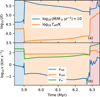 |
Fig. 1 Stellar parameters for the last 500 kyr of our evolutionary track. The blue, orange and red shading denote the MS, RSG and WR phases respectively. (a) Mass-loss rate and surface temperature vs time since ZAMS. (b) Rotation velocity, critical rotation velocity and wind velocity vs time since ZAMS. |
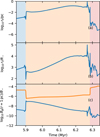 |
Fig. 2 Evolution of selected CSM magnetic field components for the last 500 kyr pre-SN. The blue, orange and red shading denote the MS, RSG and WR phases respectively. (a) Time evolution of rt, the radius where Br/Bϕ = 1 close to the equatorial plane. (b) Time evolution of rt/R⋆. (c) Time evolution of Bϕ/B⋆, where Bϕ is calculated at a distance of 1 pc from the star, for our model (blue) and with values of Zirakashvili & Ptuskin (2018) (orange). Note while R⋆ is time dependent, B⋆ is assumed to be fixed. |
2.2 MHD simulations
In this work, we performed 2D cylindrical and 3D Cartesian simulations using the MHD code PION (Mackey et al. 2021) for our models. PION includes static mesh refinement, such that high resolution can be applied in regions of interest. The entire domain D is included for refinement level n = 0, and each successive level covers D/2n. We use the evolving stellar wind source term introduced in Mackey et al. (2021).
The stellar evolution track described in Sect. 2.1 is used to obtain the star’s mass, luminosity, Teff, ![Mathematical equation: $\[\dot{M}\]$](/articles/aa/full_html/2026/07/aa57775-25/aa57775-25-eq4.png) , vrot, vesc and radius as a function of time. These parameters determine the properties of our evolving stellar wind source. Using these values as our internal boundary conditions, the system is evolved, adopting ideal MHD, as described in Mackey et al. (2021) for the pre-SN evolution. The divergence cleaning method of Dedner et al. (2002) is used throughout. The stellar magnetic field is injected as a split monopole that is swept into a spiral pattern by stellar rotation, following Mackey et al. (2021).
, vrot, vesc and radius as a function of time. These parameters determine the properties of our evolving stellar wind source. Using these values as our internal boundary conditions, the system is evolved, adopting ideal MHD, as described in Mackey et al. (2021) for the pre-SN evolution. The divergence cleaning method of Dedner et al. (2002) is used throughout. The stellar magnetic field is injected as a split monopole that is swept into a spiral pattern by stellar rotation, following Mackey et al. (2021).
Radiative heating and cooling is included following the scheme described in Green et al. (2019). We assume photoionised gas at all times, for which the heating rate is dominated by the photoionisation of recombining H+ ions. We therefore calculate the heating as the recombination rate multiplied by a mean heating energy per ionisation, assumed to be 5 eV as an average value for an O-type star (cf. Green et al. 2019). This would not be strictly true for an isolated RSG, but in a cluster environment nearby O stars would photoionise a RSG’s wind to within 0.05 pc of the star (Mackey et al. 2015; Larkin et al. 2025).
Our radiative cooling prescription (cooling model 8 in PION) includes three cooling sources, as described in Green et al. (2019). Firstly, we take the maximum of the collisional ionisation equilibrium curve for Solar metallicity described by Wiersma et al. (2009) and the forbidden-line cooling function described by Henney et al. (2009), to capture the large cooling rates in photoionisation equilibrium at T ~ 104 K. Secondly, we include Bremsstrahlung from ionised hydrogen (Hummer 1994) and helium (Rybicki & Lightman 1979). Finally, we use the hydrogen recombination cooling rate from Hummer (1994), assuming hydrogen is fully ionised. This heating and cooling prescription produces an equilibrium gas temperature T ≈ 8300 K.
We computed the RSG and WR models with different setups. For the RSG model we evolved it fully in 3D starting from the end of the MS stage of the evolutionary track. This avoids the need to wrap the CSM from 2D. For the WR model, CSM from the previous stages is important. Given the computational constraints in evolving fast stellar winds at high spatial resolution, we evolved the simulation in 2D from 2 Myr post ZAMS through the RSG stage to the end of core helium burning in 2D, and then wrapped the simulation to 3D. This is achieved using a first-order interpolation, such that the coordinates of each 3D Cartesian cell are mapped onto the 2D cylindrical grid and the scalar quantities are copied directly from the 2D grid cell into the 3D grid cell. Vector quantities from 2D such as V ≡ (vz, vR, vϕ) are transformed to Cartesian coordinates (vx, vy, vz) assuming axisymmetry.
2.3 RSG model
The evolution is performed using a 3D cubic Cartesian domain of (x, y, z) ∈ [−2.048 × 10²⁰, 2.048 × 10²⁰] cm. The 10 levels of static mesh-refinement focussed on the star at the origin give us a finest grid resolution of Δx = 3.12 × 1015 cm, or about 0.001 pc. Each refinement level has 2563 grid cells, and the factor of two refinement per level means that successive levels have domains 2× smaller along each dimension than the next coarser level. The finest level has a cubic domain (x, y, z) ∈ [−4 × 10¹⁷, 4 × 10¹⁷] cm. We choose an ambient magnetic field of (Bx, By, Bz) = (4 × 10⁻⁷, 1 × 10⁻⁷, 1 × 10⁻⁷) G. To mimic proper motion of the star, we included a small velocity for the ISM, such that in the star’s reference frame it is moving through the ISM with (vx, vy, vz) = (−4, 1, 4) km s−1. As the RSG wind would already be supersonic at rest, this small motion does not cause the wind to become supersonic, and the motion is included in order to break possible artificial symmetries that may arise from a fully stationary simulation. Inflow boundaries are set at the outer boundaries with an inflow in the initial conditions, and zero-gradient (outflow) boundaries are applied otherwise.
2.4 WR model
The WR simulation is evolved in a 2D cylindrical coordinate system (r, z) (with assumed rotational symmetry around the z axis in the angular ϕ coordinate), using a rectangular domain of r ∈ [0, 2.048 × 10²⁰] cm, z ∈ [−2.048 × 10²⁰, 2.048 × 10²⁰] cm. Ten levels of static mesh-refinement are applied, centred on the star at the origin, with a factor of two refinement between each level. Every level has 128 × 256 grid cells, and so successive levels have domain ranges 2× smaller in each dimension. The finest level has a domain r ∈ [0, 4 × 10¹⁷] cm and z ∈ [−4 × 10¹⁷, 4 × 1017 cm and a cell diameter Δx = 3.12 × 1015 cm. Axisymmetric reflecting boundary conditions are applied at r = 0, and zerogradient (outflow) conditions imposed at the outer edges of the domain. We choose a wind radius of r = 1.2 × 1017 cm, corresponding to 38 grid cells at the highest refinement level. We place the star at the origin in a uniform ISM. We choose an initial constant ambient ISM density of ρ0 = 2.338 × 10⁻²³ g cm−3, corresponding to 10 hydrogen atoms per cm3. We choose an ambient ISM pressure of P0 = 6.072 × 10⁻¹² dyne cm−3, corresponding to a temperature of 4000 K. We choose an ambient magnetic field of Bz = 4 × 10⁻⁷ G. We impose Br = 0 to avoid monopole generation on the z-axis, and Bϕ = 0 because a large-scale circular magnetic field centred on the trajectory of the star is a very unlikely configuration. The 2D axisymmetric simulation does not allow a more general magnetic field configuration that is misaligned with the grid axes, as was used above for the RSG model. We do not include proper motion as the 2D to 3D wrapping requires assuming axisymmetry, and the effects of a small proper motion would be much less pronounced with the fast WR wind.
2.5 Supernova implementation
To introduce an SN into the 3D simulation, a spherical region is over-written using an iterative two-component density and velocity profile following how Whalen et al. (2008) and Fichtner et al. (2024) implemented the solution of Truelove & McKee (1999). This profile is flat between 0 ≤ rcore and decreases sharply as a power law outside rcore to the maximum radius rmax. The power-law index we adopt is n = 9, in line with previous CCSNe simulations (e.g. Truelove & McKee 1999; Dwarkadas 2007). We choose an ejecta mass of 5 M⊙ and energy of 1051 erg (Burrows & Vartanyan 2021), giving a core velocity of 4.695 × 108 cm s−1. We chose rmax = 40 cells (~0.04 pc, corresponding to tmax ~ 1.3 yr post-explosion). This is necessary to avoid grid artefacts in the supernova remnant as it expands. Furthermore, we impose Gaussian perturbations of ±40% for each cell of the SN, to approximate an aspherical explosion. This overwriting procedure results in a small discontinuity at the leading edge of the SN which is found to smooth out within the first output timestep.
We chose a split monopole profile for our ejecta magnetic field. This decision is primarily motivated by requiring the ejecta field lines to smoothly connect to the lines already in the CSM, and our inability to simulate a convective core that would produce a physically motivated magnetic field (Varma & Müller 2021). We set the magnetic field strength such that the plasma β is equal to the β of the CSM (~100).
3 Results
We present results for our pre-SN CSM and SNR simulations, aiming to highlight differences between the RSG and WR cases arising from their different CSM. We present radial CSM profiles for both 3D SNR simulations. For the SNR simulations, we present XZ-plane slices for the density, the (normalised) compression −∇ · V/V and magnetic field strength.
3.1 Pre-SN CSM
We show key evolutionary phases of the 2D CSM in Fig. 3. The 2D and 3D CSM at the end of the RSG phase are quantitatively similar, with a large density jump at the edge of the RSG wind bubble and no MS wind bubble due to photoionisation. The ISM magnetic field is assumed to be uniform and parallel to the z-axis, and therefore spherical expansion of the wind bubble induces magnetic tension that provides a restoring force in the directions perpendicular to B but not in the parallel direction. This was explored in detail by van Marle et al. (2015), who showed that the generic solution is a bubble elongated along the axis parallel to the ISM magnetic field, and with rotational symmetry about this axis. We obtain a very similar result.
Pre-SN radial density profiles of both 3D simulations along a single exemplary ray are shown in Fig. 4. Both simulations have the expected freely expanding and shocked wind phases, separated by a WTS. These profiles are generally representative of the features in both simulations, but can be more complex for other choices of direction. For instance, multiple shells will be present for the WR model along some directions. Due to the lower mechanical luminosity during the RSG phase, the density inside the RSG model’s freely expanding wind is approximately two orders of magnitude greater than that of the WR model. The RSG wind’s density initially jumps at the WTS by the expected factor of four, but increases further with distance downstream due to radiative cooling. The density increases by a factor ≈30 beyond the WTS. In contrast to previous work (e.g. Fig. 2 of Dwarkadas (2005) and Yasuda et al. (2021)), we do not produce a thin dense shell followed by a lower density MS bubble. Instead, we observe an extended region of increasing density over ~3 pc, outside of which is the ISM. This is due to our assumption of a photoionised wind and not from omitting the MS wind, as we obtain similar results for our 2D CSM evolution including MS wind (see upper right panel of Fig. 3). When the wind and ISM are photoionised and heated to ~8000 K, the Mach number of the shocks induced by the RSG wind is much reduced, compression factor decreased, shell thickness increased and the outward-moving forward shock dissipates into a sound wave. The RSG wind bubble remains close to spherical because its expansion is subsonic and the almost-isotropic external pressure (thermal pressure dominates over dynamic and magnetic) results in an almost spherical bubble.
In both simulations, the shocked wind gas displaces ISM and stellar wind from previous evolutionary phases. In the RSG simulation this is subsonic expansion into the ISM, and so the density changes only by ~20%. In the WR simulation, the faster wind of the WR star sweeps out the residual RSG gas into a dense shell (see Fig. 3), which expands supersonically at ~100 km s−1. The dense shell is radiative and Rayleigh–Taylor (RT) unstable. The magnetic field strength inside the shell reaches peak values of 10s of μG. The dense shell driven by the WR wind is also aspherical because of the confining effect of ISM magnetic pressure.
The radial CSM profiles in our simulations differ from those presented in Garcia-Segura et al. (1996a) for both cases. In the RSG case, they produce a thin shell at the WTS at 3 pc (slow RSG wind) or 10 pc (fast RSG wind) pc, surrounded by a low-density bubble and another shell from their MS. We attribute the lack of RSG shell in our simulation to our assumption of external photoionisation, which heats the RSG wind and the ISM, reducing the Mach number (and compression factor) of the WTS and rendering subsonic the expansion into the ISM.
Our RSG WTS is at a comparable radius to their slow wind case. Direct comparison with their WR simulation is difficult due to the lack of an equivalent radial density plot. However, comparing with their Fig. 7a, qualitatively there are some differences. In their work, they have a thin WR shell, which they artificially perturb with 1% noise. They observe Vishniac instabilities (Vishniac 1983) as the dominant source of clumping, with some RT fingers as well. In our simulation, as we have wrapped a 2D CSM to 3D, we observe clumping and dynamical instabilities in the shell only in the XZ plane, as the wrapping is done in the XY plane.
The qualitative radial structure of our single star WR CSM is similar to that found by Yasuda et al. (2022). They model a binary Ib/c CCSN progenitor, where dense and slow-moving Roche-lobe overflow (RLOF) material is swept out by the subsequent WR wind, similar to the RSG material in our WR simulation. Their WR WTS and swept-up shell are both at approximately twice the radius compared to our simulation, and their swept-out shell appears to be thinner than ours. We attribute these differences to the differing stellar evolution assumptions and lack of hydrodynamic instabilities in their 1D treatment.
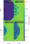 |
Fig. 3 Density slices from the 2D evolution showing the CSM during the MS (upper left), RSG phase (upper right), WR phase sweeping out the RSG shell (lower left) and pre-SN (lower right). |
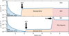 |
Fig. 4 Radial profile of density for the RSG simulation (upper panel) and WR simulation (lower panel) before the SN is inserted. The profile was calculated along a diagonal ray from the origin in the [+x, −y, +z] direction. |
3.2 RSG-SNR simulation
3.2.1 Hydrodynamic results
We evolved the simulation for 550 yr post-explosion, by which time the SNR has expanded deep into the shocked RSG wind region. We can describe the evolution of the SNR in four phases, as shown in the four panels of Figs. 5 and 6 which are slices of density and −∇ · V/V respectively.
The SNR initially expands freely into the RSG stellar wind, with its 1/r2 density profile. The stellar WTS is compressed in the direction of proper motion. The initial aspherical profile imposed in the SN explosion is quickly smoothed out as the remnant expands. A strong forward shock is established at the interface with the CSM, and a reverse shock builds up over time (~50 yr). The SNR sweeps up the RSG wind material with an approximately constant velocity, until it reaches the RSG WTS at about 1.7 pc (~230 yr). At this point the SNR has swept up an amount of mass comparable to that of the ejecta ~5 M⊙ and continues to expand. By t ~ 300 yr, the WTS has been fully swept up and the forward and reverse shocks weaken and diverge. They form two clear shells corresponding to the two shocks (~450 yr). At this point, the remnant is expanding into an approximately constant-density medium. Eventually, the reverse shock is expected to return to near the centre of explosion (e.g. Dwarkadas 2007).
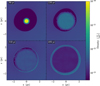 |
Fig. 5 XZ-plane slice of density for selected times of the RSG simulation. |
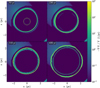 |
Fig. 6 XZ-plane slice of −∇ · V/V for selected times of the RSG simulation. |
3.2.2 Magnetic field results
In Fig. 7, we show the evolution of the magnetic field strength and orientation in a slice through the simulation. Due to the non-zero ISM velocity and slow RSG wind, a global asymmetry results leading to the SNR’s forward shock reaching the WTS at different times. The magnetic field strength increases due to compression of the frozen-in field by cooling. As the WTS is swept up, the magnetic field is compressed, reaching peak values of order 10 μG, localised in a shell of <0.5 pc thickness.
3.3 WR-SNR simulation
3.3.1 Hydrodynamic results
The WR scenario evolves the SNR for 2000 yr post explosion. The longer simulation time is necessary to observe the effects of the WR CSM, which is about a factor of two more spatially extended than the RSG case.
We describe the evolution of the SNR as shown in the six panels of Figs. 8 and 9 which are slices of density and −∇ · V/V respectively. The WR simulation begins similarly to the RSG simulation, with a free expansion phase for the first ~200 yr with the SN explosion asphericity smoothing out rapidly before reaching the WR WTS. Unlike in the RSG case, deceleration of the SNR shocks is minimal at this point due to the lower density in the freely expanding wind. After sweeping up the WR WTS, the SNR shocks continue to freely expand in the shocked wind, which is also less dense than in the RSG case. The SNR continues to expand until it hits the swept-up shell of dense RSG material at ~ 600 yr. The forward shock decelerates abruptly and reflected components travel backwards in the centre-of-explosion frame and interact with the reverse shock at ~1000 yr. The shock structure and dynamics at the RSG shell are complex until around 1400 yr post-explosion, when a coherent set of reflected shocks detach from the shell and move inwards towards the centre of explosion. As they approach the origin, a contact discontinuity develops at the RSG shell, and the forward shock continues to expand. At 2000 yr post-explosion, some of the reflected shocks are within 2 pc of the origin.
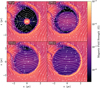 |
Fig. 7 XZ-plane slice of magnetic field strength and streamlines of in-plane magnetic field direction for selected times of the RSG simulation. |
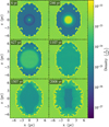 |
Fig. 8 XZ-plane slice of density for selected times of the WR simulation. |
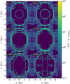 |
Fig. 9 XZ-plane slice of −∇ · V/V for selected times of the WR simulation. |
3.3.2 Magnetic field results
In Fig. 10, we show the evolution of the magnetic field strength and orientation in the XZ plane over time. In the WR simulation, the impact of including the RSG evolution can be clearly seen in the density and magnetic field structures. The SNR shock has a dense shell of RSG wind material to hit, favourable for accelerating particles, and the magnetic field strength reaches peak values of order a few 10−5 G due to radiative compression. The position of the RSG shell is relevant for potential particle acceleration, as the shock velocity decreases with shell radius (see Fig. 12). This radius will be determined by the stellar wind parameters and duration of the WR phase, as well as the external environmental conditions.
3.4 Shock properties
In this section, we examine the properties of the forward shocks in our simulations and compare with theoretical predictions. We adapted the SNR evolutionary model calculator of Leahy & Williams (2017), which uses the analytic solutions of Truelove & McKee (1999), for the timescales of interest here.
In each case, we compare from the earliest timestep until the last timestep before the forward shock encounters the WTS, where the assumptions in Truelove & McKee (1999) are no longer valid. Their model requires a constant ![Mathematical equation: $\[\dot{M}\]$](/articles/aa/full_html/2026/07/aa57775-25/aa57775-25-eq5.png) and v∞ to be assumed, so we make two comparisons. The first model takes the average of these parameters over the full duration of the preceding evolutionary stage (referred to as ‘average’) in the MESA track. The second model takes the average of these parameters over only the duration of the advection time for the preceding evolutionary stage in the MESA track, this being the last ~60 kyr for the RSG stage and the last ~1 kyr for the WR stage (referred to as ‘late’). Given the finite size rmax of the SN when initialised in our simulations, we shift the model radius values by a constant such that at tmax the radius is equal to rmax.
and v∞ to be assumed, so we make two comparisons. The first model takes the average of these parameters over the full duration of the preceding evolutionary stage (referred to as ‘average’) in the MESA track. The second model takes the average of these parameters over only the duration of the advection time for the preceding evolutionary stage in the MESA track, this being the last ~60 kyr for the RSG stage and the last ~1 kyr for the WR stage (referred to as ‘late’). Given the finite size rmax of the SN when initialised in our simulations, we shift the model radius values by a constant such that at tmax the radius is equal to rmax.
In Fig. 11, we plot the position and velocity of the forward shock in our RSG simulation inside the WTS as a function of time, alongside the average and late Truelove & McKee (1999) model predictions for a steady state stellar wind. Within this freely expanding wind region, the radial density and velocity profile of the CSM is spherically symmetric for both simulations. We show profiles along a single exemplary ray, which is representative of all directions inside the WTS. Note that the shock velocity ![Mathematical equation: $\[V_{\mathrm{sh}}=\frac{d R_{\mathrm{sh}}}{d t}\]$](/articles/aa/full_html/2026/07/aa57775-25/aa57775-25-eq6.png) is measured in the lab frame.
is measured in the lab frame.
The average values of ![Mathematical equation: $\[\dot{M}\]$](/articles/aa/full_html/2026/07/aa57775-25/aa57775-25-eq7.png) = 3 × 10⁻⁵ M⊙ yr−1 and v∞ = 28 km s−1, which are typical values for RSGs, lead to underestimates of the shock position and velocity. The late values of
= 3 × 10⁻⁵ M⊙ yr−1 and v∞ = 28 km s−1, which are typical values for RSGs, lead to underestimates of the shock position and velocity. The late values of ![Mathematical equation: $\[\dot{M}\]$](/articles/aa/full_html/2026/07/aa57775-25/aa57775-25-eq8.png) = 1.5 × 10⁻⁵ M⊙ yr−1 and v∞ = 50 km s−1 are closer to the values in the simulation. In the RSG case, we observe some additional wind acceleration from thermal pressure due to assuming photoionisation. In Fig. 12 we do the same for the WR simulation.
= 1.5 × 10⁻⁵ M⊙ yr−1 and v∞ = 50 km s−1 are closer to the values in the simulation. In the RSG case, we observe some additional wind acceleration from thermal pressure due to assuming photoionisation. In Fig. 12 we do the same for the WR simulation.
Both sets of stellar wind values (average: ![Mathematical equation: $\[\dot{M}\]$](/articles/aa/full_html/2026/07/aa57775-25/aa57775-25-eq9.png) = 2.8 × 10⁻⁵ M⊙ yr−1 and v∞= 2540 km s−1, late:
= 2.8 × 10⁻⁵ M⊙ yr−1 and v∞= 2540 km s−1, late: ![Mathematical equation: $\[\dot{M}\]$](/articles/aa/full_html/2026/07/aa57775-25/aa57775-25-eq10.png) = 2.8 × 10⁻⁵ M⊙ yr−1 and v∞ = 3100 km s−1) underestimate the radius and velocity, but only by 10–25%. We note that Truelove & McKee (1999) assume the CSM itself is static, which our results suggest leads to underestimation of the resulting shock velocities. The wind parameters in the WR stage are also more variable than during the RSG stage, and so the assumptions of a steady state and static CSM by Truelove & McKee (1999) may not be as tenable for this simulation.
= 2.8 × 10⁻⁵ M⊙ yr−1 and v∞ = 3100 km s−1) underestimate the radius and velocity, but only by 10–25%. We note that Truelove & McKee (1999) assume the CSM itself is static, which our results suggest leads to underestimation of the resulting shock velocities. The wind parameters in the WR stage are also more variable than during the RSG stage, and so the assumptions of a steady state and static CSM by Truelove & McKee (1999) may not be as tenable for this simulation.
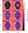 |
Fig. 10 XZ-plane slice of magnetic field strength and streamlines of in-plane magnetic field direction for selected times of the WR simulation. |
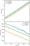 |
Fig. 11 Evolution of RSG simulation forward shock radius (upper panel) and shock velocity (lower panel) vs time up to the WTS. The profile is calculated along an exemplary diagonal ray from the origin in the [+x, −y, +z] direction. Predictions from the model of Truelove & McKee (1999) are also shown for the average and late cases as discussed in the main text. All velocities are in the centre-of-explosion frame. |
4 Discussion
4.1 Stellar evolution
In the context of particle acceleration calculations, the CSM is often approximated using an average or optimistic value for ![Mathematical equation: $\[\dot{M}\]$](/articles/aa/full_html/2026/07/aa57775-25/aa57775-25-eq11.png) and v∞. This approach is appropriate if only the freely expanding wind phase is being considered. Beyond the freely expanding wind regime, there is no such thing as a ‘typical’ CSM in terms of number, position and magnitude of features in the CSM density profile (see e.g. Fig. 4 of Fichtner et al. 2024). Different stellar evolution scenarios can generate a wide variety of different CSM density profiles. These features will mostly depend on the initial mass and multiplicity of the progenitor, and their effects on SNe have been considered by, for example, Brose et al. (2025); Das et al. (2024); Meyer et al. (2024). The latest stages of massive star evolution are the least certain, but intense, asymmetric and episodic mass-loss is expected in many cases. Given the fast WR wind advection time, we would expect qualitative differences from different WR wind prescriptions to be small, unless v∞ decreases significantly over several tens of kyr and/or
and v∞. This approach is appropriate if only the freely expanding wind phase is being considered. Beyond the freely expanding wind regime, there is no such thing as a ‘typical’ CSM in terms of number, position and magnitude of features in the CSM density profile (see e.g. Fig. 4 of Fichtner et al. 2024). Different stellar evolution scenarios can generate a wide variety of different CSM density profiles. These features will mostly depend on the initial mass and multiplicity of the progenitor, and their effects on SNe have been considered by, for example, Brose et al. (2025); Das et al. (2024); Meyer et al. (2024). The latest stages of massive star evolution are the least certain, but intense, asymmetric and episodic mass-loss is expected in many cases. Given the fast WR wind advection time, we would expect qualitative differences from different WR wind prescriptions to be small, unless v∞ decreases significantly over several tens of kyr and/or ![Mathematical equation: $\[\dot{M}\]$](/articles/aa/full_html/2026/07/aa57775-25/aa57775-25-eq12.png) changes rapidly on similar timescales. Runaway
changes rapidly on similar timescales. Runaway ![Mathematical equation: $\[\dot{M}\]$](/articles/aa/full_html/2026/07/aa57775-25/aa57775-25-eq13.png) at the end of the RSG phase (e.g. Kee et al. 2021; Bronner et al. 2025) would likely lead to significant deviations from analytical predictions based on time-averaged steady-state values for v∞ and
at the end of the RSG phase (e.g. Kee et al. 2021; Bronner et al. 2025) would likely lead to significant deviations from analytical predictions based on time-averaged steady-state values for v∞ and ![Mathematical equation: $\[\dot{M}\]$](/articles/aa/full_html/2026/07/aa57775-25/aa57775-25-eq14.png) .
.
It is not uncommon that values for ![Mathematical equation: $\[\dot{M}\]$](/articles/aa/full_html/2026/07/aa57775-25/aa57775-25-eq15.png) , vrot and B⋆ are assumed independently. However, high surface fields will impede mass-loss, and high mass-loss will lead to decreasing vrot. Using a stellar evolution model as a basis for the CSM accounts for these values simultaneously, and thus provides a greater degree of self-consistency. The lack of rapid rotation implies a radially-dominated magnetic field that falls off rapidly as B ∝ 1/r2 in this case. In this work we assume a stellar evolution track with a modest initial vrot consistent with observed Galactic O stars (Holgado et al. 2022). A fully non-rotating star would be an even less promising candidate for accelerating cosmic rays to PeV energies, which is why we did not model this scenario. Modifying the initial vrot will also affect a star’s evolutionary path, and thus the CSM and whether it explodes as a CCSN or not. Related to this, we only consider the ‘classical’ WR evolutionary scenario with single star evolution. Other formation channels for stripped-envelope SN progenitors have been suggested, invoking effects such as mass-transfer and common-envelope evolution, which would affect the CSM. Their impact on SNRs have been considered by, for instance, Ercolino et al. (2024, 2025). The structure of our WR CSM is qualitatively similar to that obtained by Yasuda et al. (2022) for a binary WR scenario, suggesting inclusion of shells of swept-up material from RSG and/or RLOF phases are important for hydrodynamic simulations of Type Ib/c in general.
, vrot and B⋆ are assumed independently. However, high surface fields will impede mass-loss, and high mass-loss will lead to decreasing vrot. Using a stellar evolution model as a basis for the CSM accounts for these values simultaneously, and thus provides a greater degree of self-consistency. The lack of rapid rotation implies a radially-dominated magnetic field that falls off rapidly as B ∝ 1/r2 in this case. In this work we assume a stellar evolution track with a modest initial vrot consistent with observed Galactic O stars (Holgado et al. 2022). A fully non-rotating star would be an even less promising candidate for accelerating cosmic rays to PeV energies, which is why we did not model this scenario. Modifying the initial vrot will also affect a star’s evolutionary path, and thus the CSM and whether it explodes as a CCSN or not. Related to this, we only consider the ‘classical’ WR evolutionary scenario with single star evolution. Other formation channels for stripped-envelope SN progenitors have been suggested, invoking effects such as mass-transfer and common-envelope evolution, which would affect the CSM. Their impact on SNRs have been considered by, for instance, Ercolino et al. (2024, 2025). The structure of our WR CSM is qualitatively similar to that obtained by Yasuda et al. (2022) for a binary WR scenario, suggesting inclusion of shells of swept-up material from RSG and/or RLOF phases are important for hydrodynamic simulations of Type Ib/c in general.
In this work, we tested stellar evolution predictions by calculating the CSM self-consistently up to the pre-SN stage, and then implementing simple explosion models to produce SNRs. This is qualitatively different to the work of Orlando et al. (e.g. 2021, 2025a,b), where detailed, tailored explosion and CSM prescriptions are used to test whether they reproduce observations of specific SNRs.
4.2 Stellar environment
Most massive stars are found in clusters. The external density and pressure from the environment can strongly affect the length scales of a star’s CSM. For example, recent JWST images of the massive young cluster Westerlund 1 show RSG winds being confined by winds of other cluster members (Guarcello et al. 2025). Red supergiants in clusters are also likely to have photoionised winds for the same reason (Mackey et al. 2015), and we show here that this leads to thicker shells with smaller compression ratios, affecting the subsequent evolution of the SNR. Red supergiants embedded in a collective cluster wind can have their own wind ablated, leading to a highly asymmetric CSM (Larkin et al. 2025). Core collapse SNe in clusters will explode into a CSM with qualitatively different properties from those in the field, and are thought to be promising sites for production of multi-PeV protons (Vieu et al. 2022).
A minority of massive stars are isolated from clusters. While it is debated whether these stars are forming in-situ (e.g. Oey et al. 2013; Oskinova et al. 2013) or are runaways from clusters (e.g. Gvaramadze et al. 2012; Vargas-Salazar et al. 2020), in either case the CSM of these stars will be qualitatively different due to the lower external densities and pressures they encounter in the field vs in a cluster. Already in our RSG simulation, the impact of a small 3D peculiar velocity is apparent in the density and magnetic field structure both pre- and post-SN. We see a compression in the WTS in the direction of motion, causing the SN to reach the WTS in this direction sooner. In the case of runaway stars with high peculiar velocities, their wind-ISM interaction produces a bow shock as the star sweeps up ISM material. This produces a strongly asymmetric CSM, as considered for example by Meyer et al. (2015, 2017).
4.3 SNR evolution
Analytic prescriptions no longer hold in the region beyond the WTS, and the effects of non-linear density structures beyond this point need to be probed via simulations. In particular, the reflected shock in our WR model processes a significant amount of energy (~3 × 1050 erg), but only occurs due to the presence of RSG shell material that is often not included in simulations (e.g. Telezhinsky et al. 2013; Zirakashvili & Ptuskin 2018). Even within the WTS, we find shock velocities faster than predicted by Truelove & McKee (1999) in both cases. For the RSG case, photoionisation produces an additional wind acceleration, and for the WR case the expansion velocity of the CSM itself is high enough to become relevant.
A consequence of our 3D treatment is our relatively poor spatial resolution at pc scales. At certain points we cannot fully resolve the complex set of interactions between different reflected and transmitted shocks. However it is clear that the forward shocks are still moving with velocities in excess of 1000 km s−1 after encountering the WTS in both cases, and therefore may be sites of non-thermal emission.
In both of our simulations, we observe enhanced magnetic field compression in the CSM from cooling. The Axford–Cranfill effect may be occurring, but given the field only increases by a factor of about two to three, it is not noticeable compared with the cooling-induced compression. The finding of B ~ r within the stellar bubble in Zirakashvili & Ptuskin (2018) is not reproduced here. The effect is also asymmetric, particularly in our RSG simulation due to the small proper motion.
Our inclusion of an aspherical explosion to break artificial symmetries did not appear to significantly affect the SNR evolution in either case, as these features were found to smooth out rapidly. A more extreme asymmetry such as a bipolar eruption would produce significant deviations, as found by, for example, Orlando et al. (2025b).
4.4 Implications for particle acceleration
The output of the simulations allowed us to consider the implications for particle acceleration, and associated non-thermal emission in young SNRs. To find the shock velocity vsh in the simulations1, we use a shock locating algorithm to determine the shock locations, and calculate the relative velocity between the fluid immediately upstream and downstream of the shock surface. The shock velocity is then
![Mathematical equation: $\[v_{\mathrm{sh}}=\frac{r}{r-1}\left(v_{\mathrm{DS}}-v_{\mathrm{US}}\right),\]$](/articles/aa/full_html/2026/07/aa57775-25/aa57775-25-eq16.png) (1)
(1)
where r is the compression ratio ρDS/ρUS, and vDS and vUS are the radial velocities downstream and upstream of the shock respectively. Defining vsh in this way is convenient when calculating the energy processed by the shock per unit time per unit area is ![Mathematical equation: $\[\frac{d E}{d t d A} \approx \frac{1}{2} \rho_{\mathrm{US}} v_{\mathrm{sh}}^{3}\]$](/articles/aa/full_html/2026/07/aa57775-25/aa57775-25-eq17.png) , where dA is a differential area element of the shock’s surface. This quantity is useful in determining the likelihood of cosmic-ray driven magnetic field amplification at the different shocks.
, where dA is a differential area element of the shock’s surface. This quantity is useful in determining the likelihood of cosmic-ray driven magnetic field amplification at the different shocks.
Forward shocks
For both the WR and RSG simulations, the shock initially expands into the CSM of the progenitor. As discussed it is the late time stellar evolution, i.e. in the ‘immediate’ pre SN period, that sets the shock and wind conditions. In this case, we can apply the method of Bell et al. (2013) (see also H.E.S.S. Collaboration 2022), to determine the maximum energy in the early phase of evolution.
We assume some fraction ηesc of the energy processed by the shock is converted to energetic protons (cosmic rays) which escape upstream, driving the growth of self-confining magnetic fluctuations as they do so (see Bell et al. 2013, for details). For the forward shock, propagating in a 1/r2 wind profile, the predicted maximum particle energy is
![Mathematical equation: $\[E_{\max }^{(\mathrm{FS})} \approx\left(\frac{\eta_{\mathrm{esc}}}{10^{-2}}\right)\left(\frac{\dot{M}}{10^{-5} \mathrm{M}_{\odot} ~\mathrm{yr}^{-1}}\right)^{\frac{1}{2}}\left(\frac{v_{\infty}}{10 \mathrm{~km} \mathrm{~s}^{-1}}\right)^{-\frac{1}{2}}\left(\frac{v_{\mathrm{sh}}}{10^3 \mathrm{~km} \mathrm{~s}^{-1}}\right)^2 \mathrm{TeV}\]$](/articles/aa/full_html/2026/07/aa57775-25/aa57775-25-eq18.png)
The above estimate assumes the escaping current produced by the accelerated protons is sufficient to drive the non-resonant current driven instability described in Bell (2004). For the simulation results presented here, i.e. using the late wind parameter values as described earlier, this equates to maximum energies in the first decade post SN of ≈100 TeV and ≈30 TeV for the RSG and WR cases respectively. Due to the evident shock deceleration the maximum energy reduces with time.
The external shocks will eventually reach the zone where enhanced magnetic field compression occurs, either due to cooling in the immediate post-shock region or, more gradually, via the Axford–Cranfill effect, should it operate. In contrast to Zirakashvili & Ptuskin (2018), we find the enhanced field regions are localised to a narrow layer beyond the transition where cooling drives strong compression. However, given the modest velocities ≈1000 km s−1 the shock retains at these locations, any effect on the maximum energy is minor. This may be due to the fact that our time-evolving value for vrot is approximately an order of magnitude lower than that of Zirakashvili & Ptuskin (2018) immediately pre-SN, and thus rt is further from the star (see panel (c) of Fig. 2). It is evident that extreme wind conditions, such as high mass loss rates with slow wind, and/or SNR conditions such as extreme shock velocities, are required for the acceleration of protons above PeV energies at the external shocks in isolated SNRs.
Reflected shocks
Since the reflected shock in the WR case processes a substantial amount of energy, we should consider here the possible radiative signatures of such a shock. Owing to the large expansion of the gas, the magnetic field strength internal to the reflected shock in the simulations is weak, B ≪ μG. A minimum requirement for excitation of the non-resonant instability is that B < BNR (Bell 2004), where
![Mathematical equation: $\[B_{\mathrm{NR}}=\left(\frac{f_{\mathrm{esc}}}{10^{-2}}\right)^{\frac{1}{2}}\left(\frac{\rho}{10^{-25} \mathrm{~g} \mathrm{~cm}^{-3}}\right)^{\frac{1}{2}}\left(\frac{v_{\mathrm{sh}}}{5000 \mathrm{~km} \mathrm{~s}^{-1}}\right)^{\frac{3}{2}} ~\mu \mathrm{G}.\]$](/articles/aa/full_html/2026/07/aa57775-25/aa57775-25-eq19.png)
Here fesc is the fraction of energy processed by the shock escaping upstream as cosmic rays flow into the SNR interior. The numerical values are motivated from the simulation results, and evidently, Bsim ≪ BNR, implying the non-resonant instability is important for magnetic field amplification at the reflected shock.
In the case of a reflected shock, its surface is converging as it moves inward, the escaping particles will thus focus towards the origin. While this may play an interesting role, a detailed model of this is beyond the scope of this work. To keep things simple, we adopt the most optimistic scenario, where the field is amplified to BNR, and assume particles reach the Hillas limit in this field. We thus set an upper limit to the maximum particle energy
![Mathematical equation: $\[\begin{aligned}E_{\text {Hillas }} & =q B R u_{\mathrm{sh}} / c \\& \approx 20 Z\left(\frac{f_{\mathrm{esc}}}{10^{-2}}\right)^{\frac{1}{2}}\left(\frac{\rho}{10^{-25} \mathrm{g} \mathrm{~cm}^{-3}}\right)^{\frac{1}{2}}\left(\frac{v_{\mathrm{sh}}}{5000 \mathrm{~km} \mathrm{~s}^{-1}}\right)^{\frac{5}{2}}\left(\frac{R_{\mathrm{sh}}}{1 \mathrm{pc}}\right) \mathrm{TeV},\end{aligned}\]$](/articles/aa/full_html/2026/07/aa57775-25/aa57775-25-eq20.png)
where again, numerical values are motivated from the simulation.
The implied low magnetic field values and modest maximum energies essentially rule out the possibility of non-thermal X-ray emission. Since the cooling time for electrons is
![Mathematical equation: $\[t_{\text {cool }} \approx 300\left(\frac{E}{1 ~\mathrm{TeV}}\right)^{-1}\left(\frac{u_{\mathrm{ph}}+u_B}{1 \mathrm{eV} \mathrm{~cm}^{-3}}\right)^{-1} ~\mathrm{kyr},\]$](/articles/aa/full_html/2026/07/aa57775-25/aa57775-25-eq21.png)
any population accelerated by the reflected shock will live long after the reflected shock has dissipated.
Let us assume the electrons are accelerated into a powerlaw energy distribution with index s ≳ 2, and a fraction ηe ≈ 0.01% of the total energy processed is given to electrons above GeV energies. In the simulation, the reflected shock processes approximately 3 × 1050 erg. If these particles are confined in the SNR interior, they may produce detectable emission in gamma rays. To estimate the gamma-ray flux, we approximate the target radiation field as a monochromatic population of photons with energy 0.1 eV with uniform energy density of 1 eV/cm3. The resulting inverse-Compton luminosity for times tSNR ≪ tcool is L(E > TeV) ≈ 1032 erg s−1, which would be detectable with current generation imaging atmospheric Cherenkov telescopes if the source was within a few kiloparsecs distance.
Prospects for CCSNe as PeVatrons
We find maximum particle energies of order a few tens of TeV for all cases considered, notably lower than was found by Zirakashvili & Ptuskin (2018) for the case of a WR progenitor for the reasons discussed above. This is broadly in line with other recent works (e.g. Brose et al. 2022), which find that extreme conditions are required to achieve PeV energies. Such possibilities include a powerful SN inside a star cluster (e.g. Härer et al. 2025), successive SNe in a superbubble (e.g. Vieu et al. 2022) or the SNR interacting with dense circumstellar material ejected shortly before explosion (e.g. Bell et al. 2013; Brose et al. 2025). Considering the reflected shock of the SNR in the WR progenitor case, the maximum energy of electrons is again found to be tens of TeV, with detectable inverse-Compton emission predicted.
5 Conclusion
In this work we computed 3D MHD simulations of young SNRs expanding through CSM generated self-consistently using a detailed stellar evolution treatment. We summarise our findings as follows:
A multi-D treatment of the CSM is required to account for the effects of dynamical instabilities on the CSM structure;
Our simulations suggest that analytic prescriptions assuming a steady-state and static CSM can underestimate forward shock velocities in young SNRs. For the RSG case, we find that photoionisation introduces an additional acceleration to the stellar wind, and for the WR case the CSM expansion velocity is also important;
Our simulations also suggest that using analytic predictions calculated with stellar wind parameters time-averaged over a full evolutionary phase are likely to be discrepant with detailed simulations if the wind parameters change significantly towards the end of the star’s life. We find time-averaging over the wind advection time to be a closer approximation in both of our cases;
Detailed stellar evolution treatment produces CSM features beyond the free-expanding wind region, which the SNR will interact with as it expands;
We show for a RSG that assuming full photoionisation, as would be expected in a young stellar cluster, produces a qualitatively different CSM. We obtain an extended region of increasing density instead of a thin dense shell at the WTS;
In agreement with previous works, we show that these interactions can produce favourable conditions for accelerating particles to a few tens of TeV, but are unlikely to reach PeV energies. We consider the particular case of a reflected shock propagating through a WR wind bubble for the first time, finding that inverse Compton emission may be detectable in gamma rays;
We demonstrate the impact of using self-consistent stellar evolution models which ensure the vrot value at explosion is consistent with the progenitor’s mass-loss history;
Cooling leads to magnetic field strengths of tens of μG at compressed regions, but we show this occurs only in thin shells, and the effects can be highly asymmetrical. We do not find the Axford–Cranfill effect to be contributing significantly in our simulations.
Acknowledgements
We thank the referee for their constructive feedback which has improved this work. The simulations presented here were performed on the HPC system Raven at the Max Planck Computing and Data Facility. CJKL gratefully acknowledges support from the International Max Planck Research School for Astronomy and Cosmic Physics at the University of Heidelberg in the form of an IMPRS PhD fellowship. This publication results from research conducted with the financial support of Taighde Eireann - Research Ireland under Grant number 20/RS-URF-R/3712. AACS is supported by the German Deutsche Forschungsgemeinschaft, DFG in the form of an Emmy Noether Research Group – Project-ID 445674056 (SA4064/1-1, PI Sander). This project was co-funded by the European Union (Project 101183150 – OCEANS). This research made use of the following software packages: Astropy (Astropy Collaboration 2018), Numpy (Harris et al. 2020), matplotlib (Hunter 2007), yt (Turk et al. 2011), PION (Mackey et al. 2021), PYPION (Green & Mackey 2021), SNR.PY (Leahy & Williams 2017).
References
- Ackermann, M., Ajello, M., Allafort, A., et al. 2013, Science, 339, 807 [NASA ADS] [CrossRef] [Google Scholar]
- Aguilera-Dena, D. R., Müller, B., Antoniadis, J., et al. 2023, A&A, 671, A134 [NASA ADS] [CrossRef] [EDP Sciences] [Google Scholar]
- Astropy Collaboration (Price-Whelan, A. M., et al.) 2018, AJ, 156, 123 [Google Scholar]
- Aurière, M., Donati, J. F., Konstantinova-Antova, R., et al. 2010, A&A, 516, L2 [NASA ADS] [CrossRef] [EDP Sciences] [Google Scholar]
- Axford, W. I. 1972, in NASA Special Publication, 308, eds. C. P. Sonett, P. J. Coleman, & J. M. Wilcox, 609 [Google Scholar]
- Bell, A. R. 2004, MNRAS, 353, 550 [Google Scholar]
- Bell, A. R. 2008, MNRAS, 385, 1884 [Google Scholar]
- Bell, A. R., Schure, K. M., Reville, B., & Giacinti, G. 2013, MNRAS, 431, 415 [Google Scholar]
- Boggs, S. E., Harrison, F. A., Miyasaka, H., et al. 2015, Science, 348, 670 [Google Scholar]
- Borkowski, K. J., Reynolds, S. P., Williams, B. J., & Petre, R. 2018, ApJ, 868, L21 [NASA ADS] [CrossRef] [Google Scholar]
- Bronner, V. A., Laplace, E., Schneider, F. R. N., & Podsiadlowski, P. 2025, A&A, 703, A61 [NASA ADS] [CrossRef] [EDP Sciences] [Google Scholar]
- Brose, R., Sushch, I., & Mackey, J. 2022, MNRAS, 516, 492 [NASA ADS] [CrossRef] [Google Scholar]
- Brose, R., Sushch, I., & Mackey, J. 2025, A&A, 699, A160 [NASA ADS] [CrossRef] [EDP Sciences] [Google Scholar]
- Burrows, A., & Vartanyan, D. 2021, Nature, 589, 29 [CrossRef] [PubMed] [Google Scholar]
- Cranfill, C. W. 1974, PhD thesis, University of California, San Diego [Google Scholar]
- Das, S., Brose, R., Pohl, M., Meyer, D. M. A., & Sushch, I. 2024, A&A, 689, A9 [NASA ADS] [CrossRef] [EDP Sciences] [Google Scholar]
- de la Chevrotière, A., St-Louis, N., Moffat, A. F. J., & MiMeS Collaboration 2014, ApJ, 781, 73 [Google Scholar]
- Dedner, A., Kemm, F., Kröner, D., et al. 2002, J. Computat. Phys., 175, 645 [Google Scholar]
- Dwarkadas, V. V. 2005, ApJ, 630, 892 [NASA ADS] [CrossRef] [Google Scholar]
- Dwarkadas, V. V. 2007, ApJ, 667, 226 [NASA ADS] [CrossRef] [Google Scholar]
- Dyson, J. E., & de Vries, J. 1972, A&A, 20, 223 [NASA ADS] [Google Scholar]
- Ercolino, A., Jin, H., Langer, N., & Dessart, L. 2024, A&A, 685, A58 [NASA ADS] [CrossRef] [EDP Sciences] [Google Scholar]
- Ercolino, A., Jin, H., Langer, N., & Dessart, L. 2025, A&A, 696, A103 [NASA ADS] [CrossRef] [EDP Sciences] [Google Scholar]
- Fesen, R. A., Milisavljevic, D., Patnaude, D., et al. 2025, ApJS, 278, 17 [Google Scholar]
- Fichtner, Y. A., Mackey, J., Grassitelli, L., Romano-Díaz, E., & Porciani, C. 2024, A&A, 690, A72 [NASA ADS] [CrossRef] [EDP Sciences] [Google Scholar]
- Frost, A. J., Sana, H., Mahy, L., et al. 2024, Science, 384, 214 [NASA ADS] [CrossRef] [Google Scholar]
- Garcia-Segura, G., Langer, N., & Mac Low, M. M. 1996a, A&A, 316, 133 [NASA ADS] [Google Scholar]
- Garcia-Segura, G., Mac Low, M. M., & Langer, N. 1996b, A&A, 305, 229 [NASA ADS] [Google Scholar]
- Ginzburg, V. L., & Syrovatskii, S. I. 1964, The Origin of Cosmic Rays (Pergamon) [Google Scholar]
- Green, S., & Mackey, J. 2021, Astrophysics Source Code Library [record ascl:2103.026] [Google Scholar]
- Green, S., Mackey, J., Haworth, T. J., Gvaramadze, V. V., & Duffy, P. 2019, A&A, 625, A4 [NASA ADS] [CrossRef] [EDP Sciences] [Google Scholar]
- Grunhut, J. H., Wade, G. A., Neiner, C., et al. 2017, MNRAS, 465, 2432 [NASA ADS] [CrossRef] [Google Scholar]
- Guarcello, M. G., Almendros-Abad, V., Lovell, J. B., et al. 2025, A&A, 693, A120 [NASA ADS] [CrossRef] [EDP Sciences] [Google Scholar]
- Gvaramadze, V. V., Weidner, C., Kroupa, P., & Pflamm-Altenburg, J. 2012, MNRAS, 424, 3037 [NASA ADS] [CrossRef] [Google Scholar]
- H.E.S.S. Collaboration (Abdalla, H., et al.) 2018, A&A, 612, A3 [NASA ADS] [CrossRef] [EDP Sciences] [Google Scholar]
- H.E.S.S. Collaboration (Aharonian, F., et al.) 2022, Science, 376, 77 [NASA ADS] [CrossRef] [Google Scholar]
- Härer, L., Vieu, T., Schulze, F., Larkin, C. J. K., & Reville, B. 2025, A&A, 703, A111 [NASA ADS] [CrossRef] [EDP Sciences] [Google Scholar]
- Harris, C. R., Millman, K. J., van der Walt, S. J., et al. 2020, Nature, 585, 357 [NASA ADS] [CrossRef] [Google Scholar]
- Henney, W. J., Arthur, S. J., de Colle, F., & Mellema, G. 2009, MNRAS, 398, 157 [NASA ADS] [CrossRef] [Google Scholar]
- Holgado, G., Simón-Díaz, S., Herrero, A., & Barbá, R. H. 2022, A&A, 665, A150 [NASA ADS] [CrossRef] [EDP Sciences] [Google Scholar]
- Hubrig, S., Schöller, M., Cikota, A., & Järvinen, S. P. 2020, MNRAS, 499, L116 [NASA ADS] [CrossRef] [Google Scholar]
- Hummer, D. G. 1994, MNRAS, 268, 109 [NASA ADS] [CrossRef] [Google Scholar]
- Hunter, J. D. 2007, Comput. Sci. Eng., 9, 90 [NASA ADS] [CrossRef] [Google Scholar]
- Jin, H., Langer, N., Ercolino, A., & de Mink, S. E. 2026, A&A, 707, A56 [NASA ADS] [CrossRef] [EDP Sciences] [Google Scholar]
- Kee, N. D., Sundqvist, J. O., Decin, L., de Koter, A., & Sana, H. 2021, A&A, 646, A180 [NASA ADS] [CrossRef] [EDP Sciences] [Google Scholar]
- Lamers, H. J. G. L. M., & Cassinelli, J. P. 1999, Introduction to Stellar Winds (Cambridge University Press) [Google Scholar]
- Langer, N. 2012, ARA&A, 50, 107 [Google Scholar]
- Larkin, C. J. K., Mackey, J., Haworth, T. J., & Sander, A. A. C. 2025, A&A, 700, A60 [NASA ADS] [CrossRef] [EDP Sciences] [Google Scholar]
- Leahy, D. A., & Williams, J. E. 2017, AJ, 153, 239 [NASA ADS] [CrossRef] [Google Scholar]
- Mackey, J., Castro, N., Fossati, L., & Langer, N. 2015, A&A, 582, A24 [NASA ADS] [CrossRef] [EDP Sciences] [Google Scholar]
- Mackey, J., Green, S., Moutzouri, M., et al. 2021, MNRAS, 504, 983 [NASA ADS] [CrossRef] [Google Scholar]
- Meyer, D. M. A., Langer, N., Mackey, J., Velázquez, P. F., & Gusdorf, A. 2015, MNRAS, 450, 3080 [NASA ADS] [CrossRef] [Google Scholar]
- Meyer, D. M. A., Mignone, A., Kuiper, R., Raga, A. C., & Kley, W. 2017, MNRAS, 464, 3229 [Google Scholar]
- Meyer, D. M. A., Velázquez, P. F., Pohl, M., et al. 2024, A&A, 687, A127 [NASA ADS] [CrossRef] [EDP Sciences] [Google Scholar]
- Meynet, G., & Maeder, A. 2005, A&A, 429, 581 [CrossRef] [EDP Sciences] [Google Scholar]
- Milisavljevic, D., & Fesen, R. A. 2013, ApJ, 772, 134 [Google Scholar]
- Nieuwenhuijzen, H., & de Jager, C. 1990, A&A, 231, 134 [NASA ADS] [Google Scholar]
- Nugis, T., & Lamers, H. J. G. L. M. 2000, A&A, 360, 227 [NASA ADS] [Google Scholar]
- Oey, M. S., Lamb, J. B., Kushner, C. T., Pellegrini, E. W., & Graus, A. S. 2013, ApJ, 768, 66 [Google Scholar]
- Orlando, S., Wongwathanarat, A., Janka, H. T., et al. 2021, A&A, 645, A66 [EDP Sciences] [Google Scholar]
- Orlando, S., Janka, H. T., Wongwathanarat, A., et al. 2025a, A&A, 696, A188 [NASA ADS] [CrossRef] [EDP Sciences] [Google Scholar]
- Orlando, S., Miceli, M., Ono, M., et al. 2025b, A&A, 699, A305 [NASA ADS] [CrossRef] [EDP Sciences] [Google Scholar]
- Oskinova, L. M., Steinke, M., Hamann, W. R., et al. 2013, MNRAS, 436, 3357 [Google Scholar]
- Owocki, S. P., & ud-Doula, A. 2004, ApJ, 600, 1004 [NASA ADS] [CrossRef] [Google Scholar]
- Paxton, B., Bildsten, L., Dotter, A., et al. 2011, ApJS, 192, 3 [Google Scholar]
- Paxton, B., Cantiello, M., Arras, P., et al. 2013, ApJS, 208, 4 [Google Scholar]
- Paxton, B., Marchant, P., Schwab, J., et al. 2015, ApJS, 220, 15 [Google Scholar]
- Paxton, B., Schwab, J., Bauer, E. B., et al. 2018, ApJS, 234, 34 [NASA ADS] [CrossRef] [Google Scholar]
- Paxton, B., Smolec, R., Schwab, J., et al. 2019, ApJS, 243, 10 [Google Scholar]
- Rybicki, G. B., & Lightman, A. P. 1979, Radiative Processes in Astrophysics (John Wiley & Sons, Inc.) [Google Scholar]
- Schneider, F. R. N., Ohlmann, S. T., Podsiadlowski, P., et al. 2019, Nature, 574, 211 [Google Scholar]
- Schöller, M., Hubrig, S., Fossati, L., et al. 2017, A&A, 599, A66 [NASA ADS] [CrossRef] [EDP Sciences] [Google Scholar]
- Shenar, T., Wade, G. A., Marchant, P., et al. 2023, Science, 381, 761 [NASA ADS] [CrossRef] [Google Scholar]
- Shu, F. H. 1992, The Physics of Astrophysics. Volume II: Gas Dynamics (University Science Books) [Google Scholar]
- Sushch, I., Le Roux, J. F., & Brose, R. 2024, in 38th International Cosmic Ray Conference, 262 [Google Scholar]
- Telezhinsky, I., Dwarkadas, V. V., & Pohl, M. 2012, A&A, 541, A153 [NASA ADS] [CrossRef] [EDP Sciences] [Google Scholar]
- Telezhinsky, I., Dwarkadas, V. V., & Pohl, M. 2013, A&A, 552, A102 [NASA ADS] [CrossRef] [EDP Sciences] [Google Scholar]
- Tenorio-Tagle, G., Rozyczka, M., & Bodenheimer, P. 1990, A&A, 237, 207 [Google Scholar]
- Tessore, B., Lèbre, A., Morin, J., et al. 2017, A&A, 603, A129 [NASA ADS] [CrossRef] [EDP Sciences] [Google Scholar]
- Truelove, J. K., & McKee, C. F. 1999, ApJS, 120, 299 [Google Scholar]
- Turk, M. J., Smith, B. D., Oishi, J. S., et al. 2011, ApJSS, 192, 9 [Google Scholar]
- van Marle, A. J., & Keppens, R. 2012, A&A, 547, A3 [NASA ADS] [CrossRef] [EDP Sciences] [Google Scholar]
- van Marle, A. J., Meliani, Z., & Marcowith, A. 2015, A&A, 584, A49 [CrossRef] [EDP Sciences] [Google Scholar]
- van Veelen, B., Langer, N., Vink, J., García-Segura, G., & van Marle, A. J. 2009, A&A, 503, 495 [NASA ADS] [CrossRef] [EDP Sciences] [Google Scholar]
- Vargas-Salazar, I., Oey, M. S., Barnes, J. R., et al. 2020, ApJ, 903, 42 [NASA ADS] [CrossRef] [Google Scholar]
- Varma, V., & Müller, B. 2021, MNRAS, 504, 636 [CrossRef] [Google Scholar]
- Vieu, T., Reville, B., & Aharonian, F. 2022, MNRAS, 515, 2256 [NASA ADS] [CrossRef] [Google Scholar]
- Vink, J. S., de Koter, A., & Lamers, H. J. G. L. M. 2001, A&A, 369, 574 [NASA ADS] [CrossRef] [EDP Sciences] [Google Scholar]
- Vink, J., Patnaude, D. J., & Castro, D. 2022, ApJ, 929, 57 [NASA ADS] [CrossRef] [Google Scholar]
- Vishniac, E. T. 1983, ApJ, 274, 152 [NASA ADS] [CrossRef] [Google Scholar]
- Wang, W., & Li, Z. 2016, ApJ, 825, 102 [Google Scholar]
- Whalen, D., van Veelen, B., O’Shea, B. W., & Norman, M. L. 2008, ApJ, 682, 49 [Google Scholar]
- Wiersma, R. P. C., Schaye, J., & Smith, B. D. 2009, MNRAS, 393, 99 [NASA ADS] [CrossRef] [Google Scholar]
- Wongwathanarat, A., Janka, H.-T., Müller, E., Pllumbi, E., & Wanajo, S. 2017, ApJ, 842, 13 [Google Scholar]
- Yasuda, H., Lee, S.-H., & Maeda, K. 2021, ApJ, 919, L16 [NASA ADS] [CrossRef] [Google Scholar]
- Yasuda, H., Lee, S.-H., & Maeda, K. 2022, ApJ, 925, 193 [Google Scholar]
- Yoon, S.-C. 2017, MNRAS, 470, 3970 [NASA ADS] [CrossRef] [Google Scholar]
- Zhekov, S. A., McCray, R., Dewey, D., et al. 2009, ApJ, 692, 1190 [NASA ADS] [CrossRef] [Google Scholar]
- Zirakashvili, V. N., & Ptuskin, V. S. 2018, Astropart. Phys., 98, 21 [Google Scholar]
Note that vsh is the flow velocity through the shock in the reference frame of the shock, as opposed to Vsh defined above, which is how fast the shock is expanding in the lab frame.
All Figures
|
Fig. 1 Stellar parameters for the last 500 kyr of our evolutionary track. The blue, orange and red shading denote the MS, RSG and WR phases respectively. (a) Mass-loss rate and surface temperature vs time since ZAMS. (b) Rotation velocity, critical rotation velocity and wind velocity vs time since ZAMS. |
| In the text | |
|
Fig. 2 Evolution of selected CSM magnetic field components for the last 500 kyr pre-SN. The blue, orange and red shading denote the MS, RSG and WR phases respectively. (a) Time evolution of rt, the radius where Br/Bϕ = 1 close to the equatorial plane. (b) Time evolution of rt/R⋆. (c) Time evolution of Bϕ/B⋆, where Bϕ is calculated at a distance of 1 pc from the star, for our model (blue) and with values of Zirakashvili & Ptuskin (2018) (orange). Note while R⋆ is time dependent, B⋆ is assumed to be fixed. |
| In the text | |
|
Fig. 3 Density slices from the 2D evolution showing the CSM during the MS (upper left), RSG phase (upper right), WR phase sweeping out the RSG shell (lower left) and pre-SN (lower right). |
| In the text | |
|
Fig. 4 Radial profile of density for the RSG simulation (upper panel) and WR simulation (lower panel) before the SN is inserted. The profile was calculated along a diagonal ray from the origin in the [+x, −y, +z] direction. |
| In the text | |
|
Fig. 5 XZ-plane slice of density for selected times of the RSG simulation. |
| In the text | |
|
Fig. 6 XZ-plane slice of −∇ · V/V for selected times of the RSG simulation. |
| In the text | |
|
Fig. 7 XZ-plane slice of magnetic field strength and streamlines of in-plane magnetic field direction for selected times of the RSG simulation. |
| In the text | |
|
Fig. 8 XZ-plane slice of density for selected times of the WR simulation. |
| In the text | |
|
Fig. 9 XZ-plane slice of −∇ · V/V for selected times of the WR simulation. |
| In the text | |
|
Fig. 10 XZ-plane slice of magnetic field strength and streamlines of in-plane magnetic field direction for selected times of the WR simulation. |
| In the text | |
|
Fig. 11 Evolution of RSG simulation forward shock radius (upper panel) and shock velocity (lower panel) vs time up to the WTS. The profile is calculated along an exemplary diagonal ray from the origin in the [+x, −y, +z] direction. Predictions from the model of Truelove & McKee (1999) are also shown for the average and late cases as discussed in the main text. All velocities are in the centre-of-explosion frame. |
| In the text | |
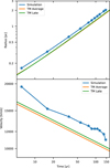 |
Fig. 12 As Fig. 11 for the WR simulation. |
| In the text | |
Current usage metrics show cumulative count of Article Views (full-text article views including HTML views, PDF and ePub downloads, according to the available data) and Abstracts Views on Vision4Press platform.
Data correspond to usage on the plateform after 2015. The current usage metrics is available 48-96 hours after online publication and is updated daily on week days.
Initial download of the metrics may take a while.