| Issue |
A&A
Volume 698, May 2025
|
|
|---|---|---|
| Article Number | A219 | |
| Number of page(s) | 6 | |
| Section | Atomic, molecular, and nuclear data | |
| DOI | https://doi.org/10.1051/0004-6361/202555275 | |
| Published online | 16 June 2025 | |
State-to-state rotational rate coefficients for the OCS+H2 collision at low temperatures
1
Departamento de Física, Facultad de Ciencias, Universidad de Chile,
Av. Las Palmeras 3425,
7800003
Ñuñoa,
Santiago
2
Facultad de Ingeniería, Universidad Autónoma de Chile,
Av. Pedro de Valdivia 425,
7500912
Providencia, Santiago,
Chile
★ Corresponding authors: otoniel.denis@uchile.cl;rodrigo.urzua@uautonoma.cl
Received:
23
April
2025
Accepted:
21
May
2025
Context. The physicochemical conditions of interstellar regions with low densities, (e.g., typical molecular clouds), should be analyzed using non-LTE models. In such models, the collisional rate coefficients of the observed molecules with H2, He, and H are critical inputs. In the case of OCS, the only set of rate coefficients available for the collision with H2 was computed in the seventies, using a potential energy surface (PES) based on an electron gas model for the collision with He. Furthermore, in a recent study on OCS+He, a mass-scaled approximation for the rates was considered, and different propensity rules were found.
Aims. The main goal of this study is to compute a new set of rotational de-excitation rate coefficients of OCS in collision with H2 at low temperatures.
Methods. An averaged PES over the orientation of H2 is developed from a large grid of ab initio energies computed at the CCSD(T)/aug-cc-pVQZ level of theory. This surface is employed in close-coupling calculations for studying the collision of OCS with para-H2(j = 0). Furthermore, an available 4D PES was also used in close-coupling calculations to confirm the results of our first approximation.
Results. The agreement between the cross sections for the OCS+para-H2 computed using the reduced and 4D PES was very good. The state-to-state rotational de-excitation rate coefficients for the lowest 30 rotational states of OCS by para-H2 are computed from these data. However, the rate coefficients show different behavior with published data; particularly, a different propensity rule, Δj = 1, is found. Furthermore, similarities between the rates with para- and ortho-H2 are found. Finally, the astrophysical implications of the new rate coefficients are explored from non-LTE radiative transfer calculations.
Key words: astrochemistry / molecular data / molecular processes / scattering / ISM: molecules
© The Authors 2025
 Open Access article, published by EDP Sciences, under the terms of the Creative Commons Attribution License (https://creativecommons.org/licenses/by/4.0), which permits unrestricted use, distribution, and reproduction in any medium, provided the original work is properly cited.
This article is published in open access under the Subscribe to Open model. Subscribe to A&A to support open access publication.
1 Introduction
In typical molecular clouds, the densities are low, and therefore, the rotational population of the interstellar species cannot be described by a Boltzmann distribution. In such cases, non-local thermodynamic equilibrium (non-LTE) models should be used to analyze the detected spectrum and determine the physicochemical conditions of the observed regions. The critical inputs of such models are the spectroscopy data, the Einstein coefficients, and the rotational state-to-sate rate coefficients of the detected molecules with the most common collider in the interstellar medium (ISM), (e.g., H2, He, H, and e−).
Carbonyl sulfide (OCS) is a widely observed interstellar molecule (Jefferts et al. 1971; Goldsmith & Linke 1981; Matthews et al. 1987; Mauersberger et al. 1995; Charnley et al. 2001; van der Tak et al. 2003; Drozdovskaya et al. 2018; Tsuge & Watanabe 2023), and the collisional rate coefficients of this species are crucial for performing non-LTE analyses. Although the interactions of OCS with He and H2 have been extensively studied in the last decades as OCS is one of the favorite probes in the study of quantum solution and microscopic superfluidity (Grebenev et al. 2000; Gianturco & Paesani 2000; Howson & Hutson 2001; Grebenev et al. 2001, 2002; Tang & McKellar 2002; Paesani et al. 2003; Tang & McKellar 2004; Yu et al. 2005; Paesani & Whaley 2004; Ross & Willey 2005; Piccarreta & Gianturco 2006; Yu et al. 2007; Michaud & Jäger 2008; Michaud et al. 2008; Grebenev et al. 2010; Li & Ma 2012; Liu et al. 2017; Oliaee et al. 2017; Raston et al. 2017; Liu et al. 2018), data with astrophysical interest are scarce. Only two sets of rate coefficients have been reported for the collision of OCS with He (Flower 2001; Denis-Alpizar et al. 2023), and one for H2 in the seventies (Green & Chapman 1978).
Green & Chapman (1978) computed the rate coefficients of OCS+para-H2 based on an electron gas potential energy surface (PES) for OCS+He, in which the long-range and minimum regions were modified, considering the long-range electrostatic interaction for OCS+H2. In our recent study of OCS+He (Denis-Alpizar et al. 2023), we compared the rate coefficients for the collisions with He and H2, and, as found by Flower (2001) before, different propensity rules were observed. Using mass-scaled rates for the collision with He to reproduce those with H2 is a common practice (Schöier et al. 2005). However, this approximation does not always work (Yazidi et al. 2014; Bop 2019), and it can predict different propensity rules (Cabrera-González et al. 2020; Urzúa-Leiva & Denis-Alpizar 2020; Tonolo et al. 2023). This appeared to be the case for OCS, and it would be valuable to confirm that from a more sophisticated PES.
Furthermore, differences up to one order of magnitude between the rate coefficients of OCS by He and H2 were observed for large |Δj| transitions (Flower 2001; Denis-Alpizar et al. 2023). Such differences were attributed by Flower (2001) to the limited number of expansion terms in the surface employed by Green & Chapman (1978) to study the collision of OCS with H2. The rates calculated for this collision were limited to transitions among the first 13 rotational states of OCS (Green & Chapman 1978); those available in the LAMDA database (van der Tak et al. 2020) for the highest values of j are just an extrapolation from their data. Therefore, a new set of accurate rate coefficients for the collision of OCS with H2 deserves to be computed.
This work focuses on the collision of OCS with H2. First, a new 2D PES for OCS-para-H2 averaged over the H2 orientation was developed. This surface was then used in close-coupling calculations for studying the collision of OCS with para-H2(j = 0). Second, an available 4D PES (Liu et al. 2017) was employed for computing rate coefficients for this system. The paper is organized as follows: In Sect. 2 the methods used are described, and in Sect. 3 the results are discussed. Lastly, Sect. 4 summarizes the main conclusions.
2 Methods
2.1 Potential energy surface
2.1.1 Reduced potential energy surface
In a first attempt, we study the collision of the OCS with para-H2, treating H2(j = 0) as a fictitious atom. This approximation has shown excellent results in the study of several collisions (Lique et al. 2008; Dumouchel et al. 2011; Desrousseaux et al. 2019; Denis-Alpizar et al. 2020). The average energy is determined from the algebraic mean of the energies at different geometrical configurations, as done by (Yazidi et al. 2014),
![$\[\begin{aligned}& E_{\mathrm{av}}\left(R, \theta_1\right)=\frac{1}{3}\left\{E\left(R, \theta_2=0^{\circ}, \theta_1, \varphi=0^{\circ}\right)\right. \\& \left.\quad+E\left(R, \theta_2=90^{\circ}, \theta_1, \varphi=0^{\circ}\right)+E\left(R, \theta_2=90^{\circ}, \theta_1, \varphi=90^{\circ}\right)\right\},\end{aligned}\]$](/articles/aa/full_html/2025/06/aa55275-25/aa55275-25-eq1.png) (1)
(1)
where the coordinates are defined in Fig. 2. Here, the angles θ1 and θ2 define the rotation of H2 and OCS, respectively; R is the distance between the centers of mass of the two molecules; and φ is the azimuthal angle.
The ab initio energies were computed at the CCSD(T)/aug-cc-pVQZ level of theory. The linear OCS was considered a rigid rotor with the interatomic distances fixed to their vibrationally averaged values in the ground state, rOC = 1.163 Å and rCS = 1.560 Å (Li & Ma 2012). For H2, the internuclear distance was also fixed to the vibrationally averaged value in the rovibrational ground state, rH–H = 0.767 Å (Jankowski & Szalewicz 1998). The grid included 30 values of R from 2.25 to 10 Å, while θ1 varies from 0° to 180° in steps of 6°. All calculations were performed with the Molpro package (Werner et al. 2012).
The analytical 2D PES was represented by using a reproducing kernel Hilbert space (RKHS) method (Ho & Rabitz 1996), such as
![$\[V\left(\mathbf{R}, \theta_{\mathbf{1}}\right)=\sum_{k=1}^N \alpha_k q^{2,5}\left(R_k, r\right) q^2\left(z_k, z\right),\]$](/articles/aa/full_html/2025/06/aa55275-25/aa55275-25-eq2.png) (2)
(2)
where N is the number of energies in the grid, ![$\[z=\frac{(1-\cos~ \theta)}{2}\]$](/articles/aa/full_html/2025/06/aa55275-25/aa55275-25-eq3.png) , and q2,5 and q2 are the radial and angular kernels as presented by Ho & Rabitz (1996). The
, and q2,5 and q2 are the radial and angular kernels as presented by Ho & Rabitz (1996). The ![$\[\alpha_{k}^{l}\]$](/articles/aa/full_html/2025/06/aa55275-25/aa55275-25-eq4.png) coefficients were obtained by solving the linear equation system Q(xk, xk′)α = V(xk), where Q(xk, xk′) = q2,5(Rk, Rk′) q2(zk, zk′). Here, k and k′ label the geometrical configurations of the grid.
coefficients were obtained by solving the linear equation system Q(xk, xk′)α = V(xk), where Q(xk, xk′) = q2,5(Rk, Rk′) q2(zk, zk′). Here, k and k′ label the geometrical configurations of the grid.
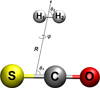 |
Fig. 1 Coordinates used to describe the OCS+H2 complex. |
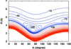 |
Fig. 2 Contour plot of the averaged 2 D PES for the OCS+H2 complex. Positive energies (red contour lines) are equally spaced in steps of 200 cm−1, while energies ≤0 cm−1 (blue contour lines) are spaced in steps of 15 cm−1. |
2.1.2 Four-dimensional potential energy surface
A relatively recent 4D PES was reported for the OCS+H2 complex by Liu et al. (2017). The description of its development can be found in (Liu et al. 2017). Briefly, this surface was computed at a high level of theory (CCSDD(T)-F12/aug-cc-pVTZ), and the coordinates employed are presented in Fig. 1. This PES was used to predict the infrared spectra of the complex(Liu et al. 2017). The comparison with experimental data validated this surface. Thus, we decided to use it in this work.
2.2 Inelastic scattering
The scattering of OCS with para-H2(j = 0) was treated in the same way as OCS+He, but using the averaged PES of Eq. (2). We employed the Newmat code (Stoecklin et al. 2002), which solves the close-coupling equation in the space-fixed frame. The log-derivative propagator (Manolopoulos 1988) was used from R = 4.0 a0 (2.1 Å), while the minimum value of maximum propagation distance was set to 40 a0 (21.17 Å) and extended automatically by the code. Sixty-four rotational states of OCS were included in the bases. At each collisional energy (Ec), the convergence of the quenching cross sections was checked as a function of total angular momentum (J). The rotational constant of OCS employed was Be = 0.20286 cm−1 (Herzberg 1966), while the centrifugal distortion constant is 4.34 × 10⁻⁸ cm−1 (Maki 1974).
The 4D PES was included in the Didimat code(Guillon et al. 2008) for studying the collision of OCS with para- and ortho-H2. This code also solves the close-coupling equations in the space-fixed frame. The log-derivative propagator Manolopoulos (1988) was employed, and the minimum distance was set at R = 4.0 a0 (2.1 Å) while the maximum propagation distance was set at 50 a0. The convergence was checked as a function of the total angular momentum for each collision energy. For the collision with para-H2, the inclusion of one and two rotational states of this species in the basis was considered. Table 1 shows the cross sections at selected collisional energies. The differences were minor (less than 10%), which we do not expect them to have a significant impact on the determination of the rate coefficients. Furthermore, considering two rotational states in the calculations increases its computational cost. Therefore, we decided to include only one rotational state of para-H2 in the basis. One rotational state was also considered in the case of ortho-H2. For OCS, we included 40 rotational states and increased this number up to 64, to ensure the inclusion of closed channels in the calculations for all cases.
Rotational cross sections of OCS for collision with H2 (in ![$\[\mathrm{a}_{0}^{2}\]$](/articles/aa/full_html/2025/06/aa55275-25/aa55275-25-eq5.png) ).
).
3 Results
3.1 Potential energy surface
Our first step in studying the OCS+H2 collision was to develop an averaged PES for the complex from Eq. (2). Figure 2 shows the contour plot for this surface. A global minimum (GM) of −127.02 cm−1 is observed at R = 3.40 Å and θ1 = 74.5°, while a secondary minima (−82.75 cm−1) is observed in the linear configuration (θ1 = 180°) at R = 4.54 Å. The geometrical configurations of the main characteristics for OCS+H2 are quite similar to those of OCS+He, where the GM (−51.69 cm−1) was at R = 3.34 Å and θ = 70.19° and the secondary minimum (−32.47 cm−1) was at R = 4.46 Å and θ = 180° (Denis-Alpizar et al. 2023).
The 4D PES (with a GM of −195.67 cm−1) of Liu et al. (2017) is deeper than our reduced surface, which is as expected since the latter is an average. Furthermore, instead of using Eq. (1) to generate the grid, we computed the energies by averaging the 4D PES over the para-H2(j = 0) rotational wave function (i.e., ⟨Yj1k V(R, θ1, θ2, φ)|Yj1k⟩ with j1 = k = 0). The behavior of this PES is similar to that shown in Fig. 2, with minimal differences that cannot be distinguished from the figures.
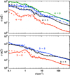 |
Fig. 3 Rotational de-excitation cross sections of OCS by para-H2(j = 0) using the 4D PES (solid lines) and the 2D PES (dashed lines). The rotational transitions of OCS are labeled as ji → jf. |
3.2 Scattering calculations
We used the 2D and 4D PES for computing the inelastic cross sections of OCS with para-H2. The bending frequency of OCS is 520 cm−1 (Shimanouchi & Shimanouchi 1980). Previous studies of the collisions of HCN and C3 with He (Stoecklin et al. 2013, 2015), which considered the bending motion of these molecules, showed that the rigid rotor is an excellent approximation for Ec values lower than the energies of the bending frequency. Therefore, the calculations were performed for collisional energies (i.e., kinetic energy) at about 150 values from 10−1 up to Ec = 500 cm−1, with a much denser grid at low collisional energies.
Figure 3 shows the cross sections (σ) computed using the 2D PES and the 4D PES. The agreement of the cross sections obtained using the 2D PES and the 4D PES is very good, with significant differences only at very low collisional energies (Ec < cm−1). These differences are expected because, at such energies, the cross sections are very sensitive to the long range of the PES, and minor differences in those regions can produce significant differences in the cross sections. Such differences have a minor impact when the cross sections are used to compute the rate coefficients. However, we decided to use the 4D PES to be able to analyze the collision with ortho-H2. Furthermore, as seen in Table 1, the values of the cross sections for the collision with He are lower than those with H2, due not only to the differences between the two PES (for the collisions with He and H2) but also to the difference in the reduced mass of the complexes.
Figure 3 also shows shape- and Feshbach-resonances typical of the van der Waals complex, which are associated with the formation of quasi-bound states due to the effective potential and the coupling between open and closed channels during a molecular collision. In addition, the cross sections globally decrease as the collisional energies increase (of course, where no resonance is involved).
The de-excitation state-to-state rate coefficients, kji → jf (T), are determined by the average of the cross sections over a Maxwell Boltzmann distribution of the collisional energy at a given temperature (T). Figure 4 shows the rate coefficients from our calculations, as well as those from Green & Chapman (1978). The rates from the collision with He (Denis-Alpizar et al. 2023), scaled as ![$\[k_{j_{i} \rightarrow j_{f}}^{H e}(T) \times 1.4\]$](/articles/aa/full_html/2025/06/aa55275-25/aa55275-25-eq6.png) (Schöier et al. 2005), were also included. The rates scaled from those for the collision with He underestimate the value from our calculations. Additionally, at a given temperature, the values decrease with increasing |Δj|. Therefore, using the scaled rates from the collision with He as a model for H2 is an approximation that should be treated with caution.
(Schöier et al. 2005), were also included. The rates scaled from those for the collision with He underestimate the value from our calculations. Additionally, at a given temperature, the values decrease with increasing |Δj|. Therefore, using the scaled rates from the collision with He as a model for H2 is an approximation that should be treated with caution.
Figure 4 also shows significant differences between the new rates and those reported by Green & Chapman (1978). These data show a propensity rule for |Δj| = 2. However, our calculations show that the difference between the rates for |Δj| = 2 and |Δj| = 1 is relatively low, particularly at the highest values of T here considered. Nevertheless, |Δj| = 1 shows greater values of the rate coefficients. The difference between the masses of C and O and the mass of S is significant. Therefore, it is not entirely surprising that OCS does not show an “almost homonuclear” behavior. Furthermore, we would like to recall that the PES from Green & Chapman (1978) was computed based on an electron gas PES for OCS–He, with modifications on the lowest four terms of the expansion of the PES to include the long-range interaction for OCS with H2.
Furthermore, we computed the rate coefficients for several initial rotational state OCS in collision with ortho-H2. Figure 5 shows the behavior of the rate coefficients from the initial j = 11 rotational states of OCS by both ortho- and para-H2 at 10 K, where a |Δj| = 1 propensity rule is also observed. This behavior is similar at other temperatures because, as seen from Fig. 4, the variation of the rates with temperature is slight above 10 K.
Similarities between the two sets of rate coefficients, with para- and ortho-H2, can also be observed in Fig. 5. Considering all the de-excitation rate coefficients from j = 3 and 4 for T between 5 K and 80 K, the averaged percent difference between the two datasets is as low as 21%. The ratio between them ranges from 0.91 to 1.29 for j = 3, and from 0.87 and 1.66 for j = 4. This behavior has been observed in other systems before: namely, HCS+ (Denis-Alpizar et al. 2022) HCO+ (Denis-Alpizar et al. 2020), N2H+ (Balança et al. 2020), SH+ (Dagdigian 2019), CF+ (Desrousseaux et al. 2019), C3N− (Lara-Moreno et al. 2019), C6H− (Walker et al. 2017), CN− (Kłos & Lique 2011), and HC3N (Wernli et al. 2007). These similarities have been attributed to the effects of long-range interactions outweighing those of short-range ones Walker et al. (2017). However, Lara-Moreno et al. (2019) found that these similarities decrease at low temperatures for C3N−, where the long-range interactions dominate the dynamics. They showed that the short-range interaction is mainly influenced by the attractive isotropic ![$\[A_{00}^{0}\]$](/articles/aa/full_html/2025/06/aa55275-25/aa55275-25-eq7.png) term, which gives nonzero contributions to the matrix element of the potential for collisions involving both para-H2(j = 0) and ortho-H2(j = 1). In the present study, these similarities are observed at very low temperatures and persist as T increases, (see Fig. 4), which suggests a combination of the two arguments: one acting at low temperatures, and the other as the temperatures increase. Therefore, we focus on the rates with para-H2.
term, which gives nonzero contributions to the matrix element of the potential for collisions involving both para-H2(j = 0) and ortho-H2(j = 1). In the present study, these similarities are observed at very low temperatures and persist as T increases, (see Fig. 4), which suggests a combination of the two arguments: one acting at low temperatures, and the other as the temperatures increase. Therefore, we focus on the rates with para-H2.
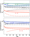 |
Fig. 4 Rotational de-excitation rate coefficients of OCS for para-H2 (solid lines) and ortho-H2 (dashed lines). The rate coefficients reported by Green & Chapman (1978) (dash-dotted lines) and those scaled from the rate coefficients with He (Denis-Alpizar et al. 2023) (dashed-double-dotted lines) are also included. The rotational transitions of OCS are labeled as ji → jf. |
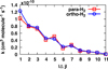 |
Fig. 5 Rotational de-excitation rate coefficients of OCS by para- and ortho-H2 for the initial rotational state of OCS j = 11 at 10 K. |
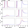 |
Fig. 6 Excitation temperature, Tex, (in K) as a function of log(nH2) (in cm−3) at two kinetic temperatures – 10 K (left panels) and 40 K (right panels) – of the gas. Solid lines correspond to the Tex determined using the rate coefficients computed in this work, while dashed lines represent those from the LAMDA database. Red and blue lines indicate column densities of 1012 and 1015 cm−2, respectively. |
3.3 Radiative transfer calculations
The discrepancies between the rate coefficients computed here for OCS+H2, and those available from the LAMDA (van der Tak et al. 2020) and Basecol databases (Dubernet et al. 2024) derived from Green & Chapman (1978) could have significant implications in the astrophysical modeling. To evaluate this impact under typical conditions of molecular clouds, we computed the excitation temperature, Tex, and the Rayleigh-Jeans equivalent temperature, TR – two quantities of astrophysical relevance – using the non-LTE radiative transfer code Radex (Van der Tak et al. 2007).
This program employs escape probability formulation under the assumption of an isothermal and homogeneous medium without large-scale velocity fields (Van der Tak et al. 2007). The calculations were performed considering the rate coefficients for OCS with H2 as it appears in the LAMDA database (van der Tak et al. 2020), and using our new rates for para-H2. The Einstein coefficients and energies of OCS are kept as they appear in the Radex data from the LAMDA database (van der Tak et al. 2020). The temperature of the background radiation field (Tcbg) was taken to be that of the microwave cosmic background field, 2.73 K, and the width of the molecular lines was set to 1.0 km s−1.
At very low densities, the radiative processes dominate, and the Tex equals the Tcbg. With an increase in the volume density, competition arises between the radiative and collisional processes. At high densities the collisions dominate, and a Boltzmann distribution can describe the rotational populations; in this case, Tex is equal to the kinetic temperature Tkin.
Figure 6 shows the Tex for several transitions of OCS at selected temperatures and column densities. In those regions where Tcbg < Tex < Tkin and where the non-LTE analysis become particularly necessary (Godard Palluet & Lique 2024), this figure shows significant deviation between the results from each dataset. At 10 K, for the 2 → 1 transition, the new rates lead to a higher Tex peak near log(nH2) ≈ 3. Similar behavior can be seen for the 4 → 3 transition at 40 K near log(nH2) ≈ 3.3. Such densities mark a regime where collisions begin to populate the upper level significantly; nevertheless, the system remains far from LTE. Furthermore, Tex becomes negative in some cases (see transitions 1 → 0 at 10 K, as well as 1 → 0 and 2 → 1 at 40 K), indicating a clear population inversion (maser-like behavior). While both datasets may predict this inversion, the critical densities at which it occurs differ.
Another quantity of interest is the TR, which can be directly compared with the observations. Figure 7 shows the ratio of TR computed from our rate coefficients and those from the LAMDA database van der Tak et al. (2020); Green & Chapman (1978) at 10 K and 40 K. At both temperatures, the new rates generally predict slightly higher TR values, especially for log(nH2) < 3. Therefore, at low densities, the ratios are higher; in such regions, the non-LTE analysis is susceptible to the rate coefficients. These results highlight the importance of using accurate collisional data for interpreting molecular observations, particularly at low densities. Therefore, we recommend employing the computed new rate coefficients, which will be available to the community through the Basecol database (Dubernet et al. 2024).
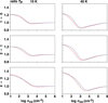 |
Fig. 7 Ratio of the TR as a function of log(nH2) (in cm−3) at two kinetic temperatures – 10 K (left panels) and 40 K (right panels) – of the gas, using the rate coefficients computed here and those from the LAMDA database. Red and blue lines indicate column densities of 1012 and 1015 cm−2, respectively. |
4 Summary
In this work, we presented a quantum study of the collision of OCS with H2. A new PES averaged over the H2 was developed and used in close-coupling calculations. The computed rate coefficients for the collision para-H2(j = 0) showed different propensity rules with available data computed about five decades ago. A relatively new published 4D PES for the OCS-H2 complex was used in close-coupling calculations, confirming the results from the averaged PES. Such different behaviors are attributed to the differences in the PES. Moreover, the rate coefficients for the collision with ortho-H2 showed similarities to those with para-H2, as observed in other collisions. This similarly is associated with the effects of long-range interactions outweighing those of short-range interactions (particularly at low collisional energies), and the influence of the short-range interaction by the attractive isotropic term which gives nonzero contributions to the matrix element of the potential for collisions involving both para- and ortho-H2.
Lastly, we computed the rate coefficients for the lowest 30 rotational states of OCS and explored the astrophysical implications of the new rates. A non-LTE analysis was performed, considering various possible conditions typical of molecular clouds. Our results show significant differences in Tex and TR when using previously available rates compared to those presented here. Such a comparison reinforces the need to incorporate up-to-date and accurate collisional data in radiative transfer models to correctly interpret molecular line observations and constrain the physical conditions of the ISM.
Data availability
The 2D PES developed in this work is publicly available on GitHub at: https://github.com/denisalpizar-group/OCS-H2_PES.
Acknowledgements
Support of project Anid/Fondecyt Regular/No. 1240102 is gratefully acknowledged. This research was partially supported by the supercomputing infrastructure of the NLHPC (ECM-02).
References
- Balança, C., Scribano, Y., Loreau, J., Lique, F., & Feautrier, N. 2020, MNRAS, 495, 2524 [Google Scholar]
- Bop, C. T. 2019, MNRAS, 487, 5685 [NASA ADS] [CrossRef] [Google Scholar]
- Cabrera-González, L., Páez-Hernández, D., & Denis-Alpizar, O. 2020, MNRAS, 494, 129 [CrossRef] [Google Scholar]
- Charnley, S., Ehrenfreund, P., & Kuan, Y.-J. 2001, Spectrochim. Acta A Mol. Biomol. Spectrosc., 57, 685 [Google Scholar]
- Dagdigian, P. J. 2019, MNRAS, 487, 3427 [Google Scholar]
- Denis-Alpizar, O., Stoecklin, T., Dutrey, A., & Guilloteau, S. 2020, MNRAS, 497, 4276 [Google Scholar]
- Denis-Alpizar, O., Quintas-Sánchez, E., & Dawes, R. 2022, MNRAS, 512, 5546 [NASA ADS] [CrossRef] [Google Scholar]
- Denis-Alpizar, O., Guerra, C., & Zarate, X. 2023, A&A, 680, A113 [NASA ADS] [CrossRef] [EDP Sciences] [Google Scholar]
- Desrousseaux, B., Quintas-Sánchez, E., Dawes, R., & Lique, F. 2019, J. Phys. Chem. A, 123, 9637 [NASA ADS] [CrossRef] [Google Scholar]
- Drozdovskaya, M. N., van Dishoeck, E. F., Jørgensen, J. K., et al. 2018, MNRAS, 476, 4949 [Google Scholar]
- Dubernet, M., Boursier, C., Denis-Alpizar, O., et al. 2024, A&A, 683, A40 [NASA ADS] [CrossRef] [EDP Sciences] [Google Scholar]
- Dumouchel, F., Kłos, J., & Lique, F. 2011, Phys. Chem. Chem. Phys., 13, 8204 [NASA ADS] [CrossRef] [Google Scholar]
- Flower, D. 2001, MNRAS, 328, 147 [CrossRef] [Google Scholar]
- Gianturco, F., & Paesani, F. 2000, J. Chem. Phys., 113, 3011 [NASA ADS] [CrossRef] [Google Scholar]
- Godard Palluet, A., & Lique, F. 2024, MNRAS, 527, 6702 [Google Scholar]
- Goldsmith, P. F., & Linke, R. A. 1981, ApJ, 245, 482 [NASA ADS] [CrossRef] [Google Scholar]
- Grebenev, S., Sartakov, B., Toennies, J. P., & Vilesov, A. F. 2000, Science, 289, 1532 [Google Scholar]
- Grebenev, S., Sartakov, B. G., Toennies, J. P., & Vilesov, A. F. 2001, J. Chem. Phys., 114, 617 [Google Scholar]
- Grebenev, S., Sartakov, B., Toennies, J. P., & Vilesov, A. 2002, Phys. Rev. Lett., 89, 225301 [Google Scholar]
- Grebenev, S., Sartakov, B. G., Toennies, J. P., & Vilesov, A. F. 2010, J. Chem. Phys., 132, 064501 [Google Scholar]
- Green, S., & Chapman, S. 1978, ApJS, 37, 169 [Google Scholar]
- Guillon, G., Stoecklin, T., Voronin, A., & Halvick, P. 2008, J. Chem. Phys., 129, 104308 [NASA ADS] [CrossRef] [Google Scholar]
- Herzberg, G. 1966, Electronic Spectra and Electronic Structure of Polyatomic Molecules (New York: Van Nostrand) [Google Scholar]
- Ho, T. S., & Rabitz, H. 1996, J. Phys. Chem., 104, 2584 [CrossRef] [Google Scholar]
- Howson, J. M., & Hutson, J. M. 2001, J. Chem. Phys., 115, 5059 [NASA ADS] [CrossRef] [Google Scholar]
- Jankowski, P., & Szalewicz, K. 1998, J. Chem. Phys., 108, 3554 [CrossRef] [Google Scholar]
- Jefferts, K., Penzias, A., Wilson, R., & Solomon, P. 1971, ApJ, 168, L111 [NASA ADS] [CrossRef] [Google Scholar]
- Kłos, J., & Lique, F. 2011, MNRAS, 418, 271 [Google Scholar]
- Lara-Moreno, M., Stoecklin, T., & Halvick, P. 2019, MNRAS, 486, 414 [CrossRef] [Google Scholar]
- Li, H., & Ma, Y.-T. 2012, J. Chem. Phys., 137, 234310 [Google Scholar]
- Lique, F., Toboła, R., Kłos, J., et al. 2008, A&A, 478, 567 [NASA ADS] [CrossRef] [EDP Sciences] [Google Scholar]
- Liu, J.-M., Zhai, Y., & Li, H. 2017, J. Chem. Phys., 147 [Google Scholar]
- Liu, J.-M., Zhang, X.-L., Zhai, Y., & Li, H. 2018, J. Phys. Chem. A, 122, 2915 [Google Scholar]
- Maki, A. G. 1974, J. Phys. Chem. Ref. Data, 3, 221 [Google Scholar]
- Manolopoulos, D. E. 1988, PhD thesis, University of Cambridge [Google Scholar]
- Matthews, H., MacLeod, J., Broten, N., Madden, S., & Friberg, P. 1987, Astrophys. J., 315, 646 [Google Scholar]
- Mauersberger, R., Henkel, C., & Chin, Y.-N. 1995, Astron. Astrophys., 294, 23 [Google Scholar]
- Michaud, J. M., & Jäger, W. 2008, J. Chem. Phys., 129, 144311 [Google Scholar]
- Michaud, J. M., Liao, K., & Jäger, W. 2008, Mol. Phys., 106, 23 [Google Scholar]
- Oliaee, J. N., Brockelbank, B., McKellar, A., & Moazzen-Ahmadi, N. 2017, J. Mol. Spectrosc., 340, 36 [NASA ADS] [CrossRef] [Google Scholar]
- Paesani, F., & Whaley, K. 2004, J. Chem. Phys., 121, 4180 [NASA ADS] [CrossRef] [Google Scholar]
- Paesani, F., Zillich, R., & Whaley, K. 2003, J. Chem. Phys., 119, 11682 [Google Scholar]
- Piccarreta, C., & Gianturco, F. 2006, Eur. Phys. J. D, 37, 93 [Google Scholar]
- Raston, P. L., Knapp, C. J., & Jäger, W. 2017, J. Mol. Spectrosc., 341, 23 [Google Scholar]
- Ross, K. A., & Willey, D. R. 2005, J. Chem. Phys., 122, 204308 [Google Scholar]
- Schöier, F. L., van der Tak, F. F. S., van Dishoeck, E. F., & Black, J. H. 2005, A&A, 432, 369 [Google Scholar]
- Shimanouchi, T., & Shimanouchi, T. 1980, Tables of Molecular Vibrational FREQUENCIES (US Government Printing Office) [Google Scholar]
- Stoecklin, T., Voronin, A., & Rayez, J. C. 2002, Phys. Rev. A, 66, 042703 [NASA ADS] [CrossRef] [Google Scholar]
- Stoecklin, T., Denis-Alpizar, O., Halvick, P., & Dubernet, M.-L. 2013, J. Chem. Phys., 139, 034304 [NASA ADS] [CrossRef] [Google Scholar]
- Stoecklin, T., Denis-Alpizar, O., & Halvick, P. 2015, MNRAS, 449, 3420 [NASA ADS] [CrossRef] [Google Scholar]
- Tang, J., & McKellar, A. 2002, J. Chem. Phys., 116, 646 [Google Scholar]
- Tang, J., & McKellar, A. 2004, J. Chem. Phys., 121, 3087 [Google Scholar]
- Tonolo, F., Bizzocchi, L., Rivilla, V., et al. 2023, MNRAS, 527, 2279 [Google Scholar]
- Tsuge, M., & Watanabe, N. 2023, Proc. Jpn. Acad., Ser. B, 99, 103 [CrossRef] [Google Scholar]
- Urzúa-Leiva, R., & Denis-Alpizar, O. 2020, ACS Earth Space Chem., 4, 2384 [CrossRef] [Google Scholar]
- van der Tak, F. F., Boonman, A., Braakman, R., & van Dishoeck, E. F. 2003, A&A, 412, 133 [NASA ADS] [CrossRef] [EDP Sciences] [Google Scholar]
- Van der Tak, F., Black, J. H., Schöier, F., Jansen, D., & van Dishoeck, E. F. 2007, A&A, 468, 627 [NASA ADS] [CrossRef] [EDP Sciences] [Google Scholar]
- van der Tak, F. F., Lique, F., Faure, A., Black, J. H., & van Dishoeck, E. F. 2020, Atoms, 8, 15 [NASA ADS] [CrossRef] [Google Scholar]
- Walker, K. M., Lique, F., Dumouchel, F., & Dawes, R. 2017, MNRAS, 466, 831 [Google Scholar]
- Werner, H.-J., Knowles, P. J., Knizia, G., Manby, F. R., & Schütz, M. 2012, WIREs Comput. Mol. Sci., 2, 242 [Google Scholar]
- Wernli, M., Wiesenfeld, L., Faure, A., & Valiron, P. 2007, A&A, 464, 1147 [NASA ADS] [CrossRef] [EDP Sciences] [Google Scholar]
- Yazidi, O., Ben Abdallah, D., & Lique, F. 2014, MNRAS, 441, 664 [NASA ADS] [CrossRef] [Google Scholar]
- Yu, Z., Higgins, K. J., Klemperer, W., McCarthy, M. C., & Thaddeus, P. 2005, J. Chem. Phys., 123, 221106 [Google Scholar]
- Yu, Z., Higgins, K. J., Klemperer, W., et al. 2007, J. Chem. Phys., 127, 054305 [Google Scholar]
All Tables
All Figures
|
Fig. 1 Coordinates used to describe the OCS+H2 complex. |
| In the text | |
|
Fig. 2 Contour plot of the averaged 2 D PES for the OCS+H2 complex. Positive energies (red contour lines) are equally spaced in steps of 200 cm−1, while energies ≤0 cm−1 (blue contour lines) are spaced in steps of 15 cm−1. |
| In the text | |
|
Fig. 3 Rotational de-excitation cross sections of OCS by para-H2(j = 0) using the 4D PES (solid lines) and the 2D PES (dashed lines). The rotational transitions of OCS are labeled as ji → jf. |
| In the text | |
|
Fig. 4 Rotational de-excitation rate coefficients of OCS for para-H2 (solid lines) and ortho-H2 (dashed lines). The rate coefficients reported by Green & Chapman (1978) (dash-dotted lines) and those scaled from the rate coefficients with He (Denis-Alpizar et al. 2023) (dashed-double-dotted lines) are also included. The rotational transitions of OCS are labeled as ji → jf. |
| In the text | |
|
Fig. 5 Rotational de-excitation rate coefficients of OCS by para- and ortho-H2 for the initial rotational state of OCS j = 11 at 10 K. |
| In the text | |
|
Fig. 6 Excitation temperature, Tex, (in K) as a function of log(nH2) (in cm−3) at two kinetic temperatures – 10 K (left panels) and 40 K (right panels) – of the gas. Solid lines correspond to the Tex determined using the rate coefficients computed in this work, while dashed lines represent those from the LAMDA database. Red and blue lines indicate column densities of 1012 and 1015 cm−2, respectively. |
| In the text | |
|
Fig. 7 Ratio of the TR as a function of log(nH2) (in cm−3) at two kinetic temperatures – 10 K (left panels) and 40 K (right panels) – of the gas, using the rate coefficients computed here and those from the LAMDA database. Red and blue lines indicate column densities of 1012 and 1015 cm−2, respectively. |
| In the text | |
Current usage metrics show cumulative count of Article Views (full-text article views including HTML views, PDF and ePub downloads, according to the available data) and Abstracts Views on Vision4Press platform.
Data correspond to usage on the plateform after 2015. The current usage metrics is available 48-96 hours after online publication and is updated daily on week days.
Initial download of the metrics may take a while.