| Issue |
A&A
Volume 699, July 2025
|
|
|---|---|---|
| Article Number | A339 | |
| Number of page(s) | 11 | |
| Section | Planets, planetary systems, and small bodies | |
| DOI | https://doi.org/10.1051/0004-6361/202553695 | |
| Published online | 17 July 2025 | |
Reduced or westward hotspot offset explained by dynamo action in atmospheres of ultrahot Jupiters
Max-Planck-Institut für Sonnensystemforschung,
Justus-von-Liebig-Weg 3,
37077
Göttingen,
Germany
★ Corresponding author: This email address is being protected from spambots. You need JavaScript enabled to view it.
Received:
7
January
2025
Accepted:
9
May
2025
Abstract
Hot Jupiters are tidally locked, Jupiter-sized planets in close proximity to their host star, exhibiting equilibrium temperatures exceeding 1000 K. Photometric observations often reveal that the hotspot - the hottest location in the atmosphere - has shifted with respect to the substellar point. While both eastward and westward offsets have been observed, hydrodynamic simulations typically predict an eastward offset due to advection by a characteristic eastward flow. In ultrahot Jupiters, where equilibrium temperatures surpass 2000 K, increased ionization has enhanced the electrical conductivity, leading to substantial Lorentz forces that can significantly influence the atmospheric dynamics. Here we present magnetohydrodynamic numerical simulations of atmospheres in ultrahot Jupiters that fully capture nonlinear electromagnetic induction effects. Our study identifies a novel magnetic instability that profoundly alters the dynamics, characterized by the disruption of the well-known laminar mean flows. This instability is triggered by a sufficiently strong background magnetic field with a realistic amplitude of around 1 G, assumed to originate from a deep-seated dynamo. Upon increasing the background field to 2.5 G, a subcritical dynamo mechanism emerges, capable of sustaining itself even when the external background field is removed. While hydrodynamic models exhibit a typical eastward offset, the magnetic instability results in either a vanishing or a westward hotspot displacement. Our results suggest that radial flow patterns associated with the instability play a significant role in modifying the hotspot position, providing a new mechanism to explain the diversity of observed hotspot shifts.
Key words: methods: numerical / planets and satellites: gaseous planets / planets and satellites: magnetic fields
© The Authors 2025
 Open Access article, published by EDP Sciences, under the terms of the Creative Commons Attribution License (https://creativecommons.org/licenses/by/4.0), which permits unrestricted use, distribution, and reproduction in any medium, provided the original work is properly cited.
This article is published in open access under the Subscribe to Open model.
Open Access funding provided by Max Planck Society.
1 Introduction
Since the discovery of the first extrasolar planet, several hundred hot Jupiters (HJs) have been found. These planets orbit their host star in close proximity and are therefore locked in synchronous rotation; they always face the same side to the star. Two observations characterize the potential impact of the atmospheric dynamics on the temperature structure: the offset of the brightness maxima from the substellar point (hotspot or phase curve offset) and the difference between dayside and nightside temperatures (e.g. Parmentier & Crossfield 2018; Bell et al. 2021; May et al. 2022).
Early observations indicated that hotspots have shifted eastwards (in the prograde direction) from the substellar point (Harrington et al. 2006; Cowan et al. 2007; Knutson et al. 2007) and that the dayside-to-nightside temperature difference is reduced. Both fit well with the action of a fast eastward-directed jet predicted by hydrodynamic theory (e.g., Showman & Polvani 2011), shallow general circulation models (e.g., Showman & Guillot 2002; Heng et al. 2011; Rauscher & Menou 2012; Cho et al. 2015), or hydrodynamic simulations (e.g., Dobbs-Dixon & Lin 2008; Dobbs-Dixon & Agol 2013). Such a jet would simply advect the temperature structure in an eastward direction, and the dynamics would transport heat from the dayside to the nightside, thereby reducing the temperature difference (see Showman et al. 2020, for a review).
However, more recent observations (Bell et al. 2021; May et al. 2022) show that both eastward and westward hotspot offsets can occur with no clear dependence on the equilibrium temperature or rotation period (see Table 1). Possible explanations include reflections from an inhomogeneous cloud layer (Parmentier et al. 2016; Roman & Rauscher 2017), asynchronous rotation (Rauscher & Kempton 2014), or magnetic effects.
From theory and earlier work, two important magnetic dynamical regimes are expected that are distinguished by the impact of the Lorentz force (e.g., Rogers & Komacek 2014; Dietrich et al. 2022). In the strong-Lorentz-force regime, the Lorentz force provides the dominant saturation mechanism by altering the flows. In the weak-Lorentz-force-regime, however, the magnetic field growth is saturated by magnetic dissipation. The Lorentz force not only increases with electrical conductivity (larger temperatures) but also with the amplitude of an assumed background field.
While some authors model the impact of the Lorentz force on the flows with a simple linear magnetic drag (Perna et al. 2010; Rauscher & Menou 2013; Beltz et al. 2022), a fully nonlinear treatment of the dynamics and magnetic field generation seems more appropriate at higher equilibrium temperatures. Such an approach was taken by Rogers & Komacek (2014), who explored the dynamics in the outer stably stratified part of HJ atmospheres with equilibrium temperatures of up to about 2000 K (at 0.01 bar). Imposing magnetic fields with strengths of up to 30 G, they report that magnetic effects become important beyond about 1500 K where electrical conductivities of about 0.01 S/m are reached. The magnetic effects can then yield highly variable and at times even westward zonal flows in the equatorial region. This may explain the different offset values observed for HAT-P-7b (Rogers 2017). Rogers & McElwaine (2017) further explore a model with an equilibrium temperature of 1800 K from Rogers & Komacek (2014) by adding lateral variations in conductivity that reflect a temperature difference of 1000 K between the substellar point and the opposing point on the nightside, causing a conductivity difference of about two orders of magnitude. Compared to a model with a constant base conductivity of about 0.02 S/m, the additional variation seems to promote dynamo action since the magnetic effects still survives when the background field is switched off.
Hindle et al. (2019) and Hindle et al. (2021b) further explore the role of magnetic effects in a simplified shallow-water model, using a prescribed azimuthal magnetic field. They demonstrate that Lorentz forces can indeed lead to westward equatorial flows, and thus a westward hotspot offset, provided the prescribed field and/or the assumed temperature are high enough.
The ability of a flow to generate magnetic fields depends on the nondimensional magnetic Reynolds number,
 (1)
where μ0 is the magnetic permeability, σ the electrical conductivity, U a typical velocity, and R the planetary radius. The magnetic Reynolds number quantifies the ratio of magnetic-field induction to magnetic-field dissipation.
(1)
where μ0 is the magnetic permeability, σ the electrical conductivity, U a typical velocity, and R the planetary radius. The magnetic Reynolds number quantifies the ratio of magnetic-field induction to magnetic-field dissipation.
Simulations and observations indicate jet velocities, U, on the order of kilometer per second (Showman et al. 2020; May et al. 2021). The temperatures in the outer atmospheres of HJs are high enough to ionize alkali metals. Below about 2400 K, the conductivity strongly increases with temperature (e.g., Dietrich et al. 2022; Kumar et al. 2021). However, in a range between 2400 K and 3600 K, this dependence levels off at values of approximately 1 S/m (Kumar et al. 2021; Dietrich et al. 2022). The reason is that these temperatures are high enough to fully ionize alkali metals but not yet high enough to ionize hydrogen. Assuming U = 1 km/s, σ = 1 S/m and a planetary radius of R = 1.2RJ yields huge magnetic Reynolds numbers on the order of Rm ≈ 105. At such large values, strong magnetic fields could be generated and would impact atmospheric dynamics (Dietrich et al. 2022).
Here, we perform magnetohydrodynamic simulations for the atmosphere of so-called ultrahot Jupiters (UHJs) with equilibrium temperatures beyond 2000 K where the electrical conductivity is particularly high. For simplicity we assume a constant electrical conductivity. Varying the amplitude of the imposed background field, we find a new magnetic instability that has a strong impact on the dynamics and yields a reduced or even westward hotspot shift.
2 Methods
2.1 Fundamental equations
We modeled the flow and entropy evolution and the magnetic field generation in a rotating and stably stratified UHJ atmosphere that is subject to a permanent irradiation with the magnetohydrodynamic code MagIC (Wicht 2002; Gastine & Wicht 2021; Lago et al. 2021). The implementation of stable stratification builts on the work of Dietrich & Wicht (2018) and Gastine & Wicht (2021). It is of great advantage to treat motion and magnetic field generation as disturbances around a background state. Following a classical approach, MagIC assumes a hydrostatic and adiabatic background state.
MagIC adopts a nondimensional formulation, using the inverse rotation rate, Trot = Ω−1, as a timescale, the spherical shell thickness, D = ro - ri, between the inner radius, ri, and outer radius, ro, as a length scale,  as a magnetic scale, and D(dSc/dr) as an specific entropy scale, where (dSc/dr) is the entropy gradient responsible for driving motions. The momentum Equation (2), energy Equation (3), and induction Equation (4) then read:
 (2)
(2)
 (3)
(3)
 (4)
(4)
Bold symbols indicate vectors, with the velocity being denoted by u and the magnetic field by B. A modified pressure is denoted by p and the specific entropy perturbation by S.t is time and er the radial unit vector. The rate-of-strain tensor, stress tensor, and viscous heat production are given by the following expressions in Cartesian coordinates:
 (5)
(5)
 (6)
(6)
![Mathematical equation: \begin{align} \Phi_\nu &= 2\tilde\rho\left[e_{ij}e_{ji}-\dfrac{1}{3}\left(\vec{\nabla}\cdot\vec{u}\right)^2\right]. \end{align}](/articles/aa/full_html/2025/07/aa53695-25/aa53695-25-eq8.png) (7)
(7)
The set of Equations (2) to (4) was complemented by the continuity equation for the mass flux and by the solenoidal condition for the magnetic field:
 (8)
(8)
To ensure these conditions, MagIC decomposed the mass flux and the magnetic field into poloidal and toroidal contributions. For example, the mass flux is given by
 (9)
where W and Z are poloidal and toroidal potentials, respectively.
(9)
where W and Z are poloidal and toroidal potentials, respectively.
The system is controlled by the nondimensional Rayleigh number, Ra, Prandtl number, Pr, magnetic Prandtl number, Pm, Ekman number, Ek, and aspect ratio, a:
 (10)
(10)
 (11)
(11)
 (12)
(12)
 (13)
(13)
 (14)
(14)
Here, cp is the specific heat capacity at constant pressure, α the thermal expansivity, ν the kinematic viscosity, κ the thermal diffusivity, and λ = 1/(μ0σ) the magnetic diffusivity.
The background state, which depends only on the radius and is characterized by quantities with a tilde, was assumed to be stationary, close to being adiabatic, and nonmagnetic. The background density, ρ̃, background temperature, T̃, and background gravity, g̃, were nondimensionalized with their outer-boundary reference values, ρo, To, and go. The Rayleigh number, Ra, scales the buoyancy due to deviations from the background state. These deviations are responsible for driving any motions. An additional stratification parameter, A, is necessary to introduce the stable stratification:
 (15)
(15)
A has been nondimensionalized with dSc/dr.
The radial profiles of background temperature and density are then given by
 (16)
(16)
The parameter εs, the dissipation number, Di, and the polytrope index, n, are further dimensionless parameters that control the background state. While εs scales the deviation from adiabaticity,
 (17)
(17)
Di is defined as
 (18)
(18)
For the gravity profile, we assumed that most of the mass is concentrated underneath the region of interest, which then yields
 (19)
(19)
The term in the entropy Equation (3) that describes radial motion along the background entropy gradient ensures that buoyancy is reduced for outward motion but increased for inward motion. The Newtonian cooling term in the entropy equation,
 (20)
(20)
models the one-sided stellar irradiation and is the only direct driver of motion. It drives the system back to the equilibrium entropy pattern, Seq, shown in Fig. 1 that reflects the irradiation on the day side and cooling to space on the night side:
 (21)
(21)
Here β(θ, φ) is the angle between the radial vector, er(θ, φ), and the vector pointing towards the substellar point, er(π/2,0). The maximum of Seq is SN, while the mean value vanishes. The specific choice of amplitudes guarantees that the mean entropy flux vanishes.
The radiative timescale, τrad(r), serves to control the impact of the radiation in the system. It rapidly increases with depth to reflect the limited penetration of the stellar radiation. We assumed a dependence such as
 (22)
(22)
similar to the one suggested by Iro et al. (2005, Fig. 4). The radiative timescale at the outer boundary, τo, is then the dimensionless parameter that measured the impact of stellar irradiation.
As entropy boundary conditions we used the fixed radial gradient. Stress-free and impenetrable inner and outer boundaries were assumed for the flow. The magnetic field was matched to a potential field at both boundaries.
The numerical method is in principle similar to the anelastic formulation used by Rogers & Komacek (2014). We employed the MagIC code (version 5.8, see Wicht 2002; Lago et al. 2021), which has been benchmarked against other anelastic codes (Jones et al. 2011) and extensively used for simulating shells with a partly stable stratification (e.g., Dietrich & Wicht 2018; Gastine & Wicht 2021; Wulff et al. 2022; Wulff 2023). As a pseudo-spectral code, MagIC is based on a spherical harmonic transform in the horizontal direction and on a decomposition in Chebychev polynomials in the radial direction. More details can be found in Wicht (2002), Gastine & Wicht (2021), and Lago et al. (2021).
We used hyperdiffusion to damp away some very small-scale spurious modes, a phenomenon that has apparently also been observed by Rogers & Komacek (2014). The hyperdiffusion only acts on the flow and is implemented as a factor, d(ℓ), acting on the kinematic viscosity,
![Mathematical equation: d(\ell)=1+D\left[\frac{\ell+1-\ell_{hd}}{\ell_{\rm{max}}+1-\ell_{hd}} \right]^{\beta},](/articles/aa/full_html/2025/07/aa53695-25/aa53695-25-eq24.png) (23)
(23)
for all spherical harmonic degree ℓ ≥ ℓhd, where we used ℓhd = 100, β = 1.5, and D = 100. Our simulations resolve spherical harmonic degrees until ℓmax = 170, using 512 equidistant grid points in longitude, 256 grid points in latitude, and 73 radial grid points on a Chebychev grid.
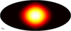 |
Fig. 1 Dimensionless equilibrium entropy pattern, Seq, used to model the stellar irradiation in the Newtonian cooling scheme (see Equations (20) and (21)). |
2.2 Model atmosphere
Table 1 lists UHJs with equilibrium temperatures of about 2200 K or higher for which a hotspot shift has been observed. Our model is supposed to cover the outer atmosphere region where the dynamic transitions from being clearly irradiation-dominated to being ruled by the flow. This roughly happens in the layer between 0.01 bar and 1 bar, which we assume to occupy roughly the outer 15% in radius.
The nondimensional numbers are based on observables and on material properties. In particular the transport properties are hard to estimate. For the kinematic viscosity, ν, we assumed a value of 10−6 m2/s that was calculated with ab initio methods for the 1 bar level of Jupiter (French et al. 2012) and of some exoplanets (Becker et al. 2018). Column 11 of Table 1 shows that this yields Ekman numbers with values of about
 (24)
(24)
The Ekman number measures the importance of viscous drag for the dynamics. Such a small value is typical for the dynamics of planetary atmospheres.
Doppler measurements of zonal winds on HJs (Snellen et al. 2010) suggest velocities with speeds reaching kilometer per second, which means that the rotational timescale and flow timescale, τU = RHJ/U, become comparable. The Rossby number, the ratio of both timescales, can thus reach unity:
 (25)
(25)
The Rossby number quantifies the impact of the Coriolis force on the dynamics and is thus important for characterizing the dynamic regime. For UHJs explored here we thus expect that the Coriolis force may not dominate.
Column 12 in Table 1 list magnetic Reynolds numbers for a velocity of 1 km/s and an electrical conductivity of 0.5 S/m, which is more appropriate for the dayside. Rather extreme magnetic Reynolds number of
 (26)
(26)
are reached.
The degree of stable stratification is typically quantified by the ratio of the Brunt-Väisälä frequency, N, and the rotation rate, Ω. While N provides the timescale of buoyancy restoring forces, the dynamic stiffness in rotating systems is determined by the Coriolis force and thus scales with Ω. For the ideal gas assumed here, the quadratic Brunt-Väisälä frequency is then given by
 (27)
(27)
On the dayside, HJs develop a nearly isothermal outer atmospheric region, which suggests a crude estimate for the stratification:
 (28)
(28)
Adopting cp = 104 J/(kg K), again from French et al. (2012) calculated for Jupiter , yields the values of the stratification listed in column 13 of Table 1:
 (29)
(29)
The extremely large value for KELT-1b reflects its high mass, which is equivalent to about 27 Jupiter masses. We have used the equilibrium temperature, which assumes radiation from dayside and nightside, and for simplicity have assumed that the stratification is the same all over the planet.
The thermal diffusivity is even harder to estimate than the kinematic viscosity. While the electronic thermal diffusivity rapidly decays in the outer layers of the models calculated by French et al. (2012) for Jupiter and Becker et al. (2018) for exoplanets, the ionic thermal diffusivity increases with decreasing pressure and seems to take over. Here we assume a value of κ = 10−4 m2/s but note that this is highly uncertain. The Prandtl number is then
 (30)
(30)
Since our adopted electrical conductivity yields a magnetic diffusivity of λ = 1/(μ0σ) ≈ 106 m2/s, the magnetic Prandtl number is
 (31)
(31)
Properties and parameters for UHJs with known hotspot shift.
2.3 Choice of numerical parameters
Some concessions are necessary for simulating the dynamics of the UHJ atmosphere with the available numerical resources. Since it is impossible to run numerical models where all parameters assume realistic values, we rather aim to choose parameter combinations that guarantee a realistic dynamic regime.
We assume that the considered part of the atmosphere has a thickness of 0.15 RHJ, and thus an aspect ratio of a = 0.85. For the Newtonian forcing pattern, we chose SN = 3.33. The radiation timescale, τo, which scales the impact of the Newtonian forcing, was chosen such that its outer boundary value was ten times smaller than the rotational time scale, i.e., τo = 0.1. For our selected UHJs, this amounts to about 104 s, which is consistent with the value suggested by Iro et al. (2005) for a pressure of 0.01 bar. This guarantees that the outer boundary of the system remains very close to the equilibrium entropy distribution shown in Fig. 1. The choice determines the position of our outer boundary in a planet. Since our model covers a pressure change by two orders of magnitude, the lower boundary simply correspond to the radius where the pressure reaches about 1 bar.
The radiation timescale rapidly increases with depth and already reaches a value comparable to the rotation timescale at a radius of r = 0.954ro. This is the radius at which we expect the flow starts to play a significant role for hotspot shift and heat advection, equilibrating dayside and nightside temperatures.
Since MagIC solves for small disturbances around an adiabatic background state, we used a small adiabaticity parameter of εs = 10−4 . The choice of density profile was limited by the available numerical power. Using a polytropic index of n = 2 and a dissipation number of Di = 3 yields a density variation of  density scale heights, which corresponds to a density contrast of about 20. We chose a polytropic background state with polytrope index n = 2 to gain a pressure increase of two orders of magnitude across the shell.
The limited computing power also forces one to choose a larger kinematic viscosity than is appropriate to damp smaller scales that cannot be resolved. Therefore, our Ekman number of Ek = 10−4 is much higher than the typical value of Ek = 10−17 estimated for our selected UHJs. The Rayleigh number needs to be adjusted to the larger Ekman number to guarantee that the simulations run in an appropriate dynamical regime. We chose a value of Ra = 108, which yields maximum wind velocities that correspond to a Rossby number of Ro ≈ 0.6, close to the outer boundary in our nonmagnetic simulation.
Adopting the very small realistic magnetic Prandtl number would result in no dynamo action. Instead, we chose the value of Pm = 0.16, which yields a magnetic Reynolds number in the range predicted for the dayside of the considered exoplanets:
 (32)
(32)
The adopted Prandtl number, on the other hand, has the realistic value of Pr = 0.1.
We chose A = 100 for the radial entropy gradient of the stable stratification, which translates to
 (33)
(33)
While this guarantees a strong degree of stratification, the estimates listed in Table 1 predict significantly higher values for some UHJs.
As was mentioned above, the magnetic field was solved for in units of  . The square of the magnetic field amplitude is then the Elsasser number:
 (34)
(34)
The Elsasses number is a measure for the ratio of Lorentz to Coriolis force in the Navier-Stokes equation. For values of Λ ≥1, we expect a strong impact of Lorentz forces on the dynamics.
In order to rescale the dimensionless results to physical values and vice versa, we have to assume a value for the outer boundary reference density, ρo. Using T = 2400 K and assuming pure hydrogen yields ρo ≈ 10−4 kg/m3 for an ideal gas. The factor to rescale the dimensionless simulations to field strengths given in Gauss then becomes  for our selected UHJs when using our assumed conductivity of σ = 0.5 S/m. Note that the rescaling is complicated by the fact that we neglected any radial or horizontal variation in the electrical conductivity, σ.
3 Results
3.1 Flows and magnetic fields
We started our exploration with a pure hydrodynamic case and then imposed a magnetic axial dipole of varying strength, Bint, representing the field produced by an interior dynamo process. Field strengths of Bint = 0.0025 G, 0.025 G, 0.25 G, 1.0 G, and 2.5 G were tested, which roughly lie in the range suggested for HJs. For example, the scaling relation by Dietrich et al. (2022) predicts upper field strengths between 7 and 11 Gauss for a planet with a 20% larger radius and a 30% larger mass than Jupiter, assuming an age range between 0.1 and 4.5 Gys (compare also to Batygin & Stevenson 2010; Yadav & Thorngren 2017). The axial dipole is imposed as a boundary condition at the lower boundary of the simulation domain. All other poloidal field contributions fulfill the usual potential field condition. Each simulation was integrated for about a viscous dissipation time to ensure that a statistically steady state was safely reached. This corresponds to 104 rotations for the Ekman number of 10−4 chosen here. During the initial phase, the imposed field dissipates into the shell while being modified by the flow.
Figure 2 shows maps of entropy (top row) and the three flow components (rows 2-4) slightly below or at the outer boundary. Depicted are snapshots at the end of the integration for the three Bint values 0.0025 G, 1.0 G, and 2.5 G. They correspond to Elsasser numbers of Λint = 0.0007, 1, and 6.8, spanning a range where the Lorentz force is expected to have a negligible to a very large impact on the dynamics. Figure 3 illustrates the time evolution of kinetic and magnetic energies for the three selected background field strengths. While times smaller than zero show the evolutions with an imposed field, times larger than zero illustrate the evolution after the axial dipole background field imposed at the lower boundary, ri, has been switched off at t = 0. This procedure allows one to determine whether the setup continues to operate as a self-consistent dynamo.
In Figure 4, we compare time averaged kinetic and magnetic energy spectra (top row) and root-mean-square (rms) force spectra (bottom row, following Aubert et al. 2017; Schwaiger et al. 2019) for the selected background field strengths. We distinguish between toroidal contributions for field lines or flows closing on spherical shells and the remaining poloidal contributions, which contain a radial component. Axisymmetric zonal flows or fields are purely toroidal, while axisymmetric radial or latitudinal (meridional) flows or fields are purely poloidal.
We start by discussing the evolution with a maintained background field. For the weakest field, the hotspot offset and velocity field are virtually indistinguishable from the purely hydrodynamic solution (left column in Figure 2). The flow is very similar to the typical solutions found in general circulation models (Showman & Guillot 2002; Heng et al. 2011; Rauscher & Menou 2012). The hotspot (first column, first row) has shifted towards the east due to an eastward zonal flow (second row, red) in the equatorial region. The non-axisymmetric flows are dominated by one horizontal large-scale cyclonic circulation cell in each hemisphere, which is anticyclonic in the northern and cyclonic in the southern hemisphere. These cells can best be discerned in the latitudinal flow (row 3), centered around 30 degrees longitude prograde of the substellar point, and are about one order of magnitude slower than the zonal flows. The radial flows (Figure 2, first column, row 4) are again more than an order of magnitude slower and show a large-scale pattern of up- and down-flows, which has slightly shifted with respect to the substellar point. Panel a in Figure 3 demonstrates that the flow becomes essentially stationary with slow variations on the viscous timescale that amount to only roughly 5% in kinetic energy and are thus hard to discern in the figure. The magnetic energy (same panel) becomes also quasi-stationary (for t < 0) and remains much smaller than the kinetic energy.
Figure 4a shows that the large-scale magnetic energy is at least three orders of magnitude lower than the kinetic energy. Smaller-scale toroidal contributions for spherical harmonic degrees beyond 20, however, become comparable. The spectra of the different force contributions, shown in Figure 4d, illustrate that the primary balance is between the buoyancy, pressure gradient, and Coriolis force. Advection (inertia) comes in at a secondary level, while viscous and Lorentz forces are again much smaller.
The first panel in the bottom row of Figure 2 shows that the radial magnetic field is significantly altered from the imposed axial dipole. Strongly localized thin stripes are produced around the equatorial plane and connect the equatorial plane with the poles. A similar pattern also appears in the azimuthal field (row 5). In order to understand the origin of this complex structure, we analyzed the time evolution right after the internal field was imposed. The initial changes result from shearing and advecting the background axial dipole. The growing induced field progressively assumes a structure that seeks to avoid shear. In other words, the induction term,  , is minimized since B and u become almost parallel. In the saturated phase, the remaining induction is balanced by dissipation. For the toroidal field, dissipation plays a larger role than for the poloidal field.
When the imposed field is so weak that Lorentz forces cannot influence the flow, field saturation can be achieved by a balance between the induction and Ohmic dissipation. The induced field should then scale like (Wicht et al. 2019; Dietrich et al. 2022):
 (35)
(35)
We find that this linear scaling indeed roughly applies for the maximum toroidal field strength in our cases with Bint = 0.0025 G, Bint = 0.025 G, and Bint = 0.25 G where the flows have hardly changed, and the magnetic field structure also remains very similar.
While the linear scaling is typically expected when Rm(D/ro) < 1, it still holds for our much larger value of Rm(D/ro) = 6300 since the background field is weak. The scaling for the poloidal field is different because the weaker non-axisymmetric flows play an important role, creating a complex field structure that avoids the shear and thereby minimizes induction. The poloidal field strength nevertheless scales linearly with the background field strength for Bint ≤ 0.25 G but at a lower level than is predicted by Equation (35).
When the background field has reached a strength of 1.0 G, the solution changes drastically. Figure 4b shows that kinetic and magnetic energies now have a similar spectrum and reach comparable magnitudes. Figure 4e demonstrates that the Lorentz force becomes comparable to the Coriolis force for harmonic degrees one and two and even exceeds it at degrees beyond 10. Consequently, the Lorentz force significantly alters the flow.
The zonal wind (Figure 2, middle column, second row) underneath and west of the hotspot is reduced by about a factor of two and assumes a wavy pattern. The entropy structure at r = 0.98 ro (third column, first row) reflects the changed flow, showing a fuzzier structure and a vanishing hotspot shift (see discussion below). Latitudinal (row 3) and radial (row 4) flows increase in amplitude and develop small-scale disturbances. Non-axisymmetric and time-dependent features now have a magnitude comparable to the axisymmetric zonal flows. The toroidal and poloidal magnetic fields have been significantly amplified and both are locally much larger than the imposed dipole (bottom three panels of the middle column in Figure 2). The field structure becomes localized and very complex.
Panel b in Figure 3 demonstrates that the toroidal kinetic energy has decreased by more than an order of magnitude compared to the cases with weaker or no imposed field. The poloidal kinetic energy, on the other hand, slightly increases. Moreover, kinetic and magnetic energy vary by a few percent, apparently chaotically, on timescales of the order of 10 rotation periods. We interpret the changes in flow and magnetic field as the onset of an instability, as is further discussed below.
When increasing the background field to 2.5 G, the Lorentz force is even stronger and promotes strong and complex space-and time-dependent features. This solution, which is already to a lower degree apparent for the 1 G background field, presents a completely new dynamical regime for the dynamics of exoplanet atmospheres that has never been described before. The Lorentz force is comparable to or larger than the Coriolis force at all scales (Fig. 4f). Both toroidal and poloidal magnetic energy exceed their kinetic counterparts (Figs. 3c and 4c).
The influence of the magnetic field is so strong that the zonal flows become unstable and the solution assumes a highly complex and turbulent nature. Azimuthal flows develop a fuzzy structure at nearly all latitudes (second row, last column of Figure 2). A band of prograde zonal wind is still the strongest flow in the domain, but this band is completely interrupted at some longitudes. The entropy structure at r = 0.98 ro (first row, last column) is now even fuzzier and shows no apparent hotspot shift.
The radial magnetic field shows a very localized disrupted structure (last column, bottom row in Figure 2). Its strength reaches typical values around 2 G and a maximum value around 10 G and is thus clearly stronger than the imposed background field. The azimuthal field (row 5) reaches typical values of 15-20 G and a huge maximum value around 80 G (Fig. 2i).
To test whether the imposed background fields were strong enough to initiate a subcritical dynamo, we switched off the background field after the simulations had reached a statistically steady state. Subcritical dynamos only work when the magnetic field is strong enough to change the flow in a suitable way. Once the locally produced field had reached a sufficient amplitude, a subcritical dynamo could be maintained even after the imposed field had been switched off. The time evolution of the kinetic and magnetic energies of these test runs are shown in Figure 3 where the background field has been switched off at t = 0. The solutions were then integrated for more than 8000 rotations.
Panel a of Figure 3 illustrates that the poloidal magnetic energy first decays somewhat faster and then purely exponentially with an imposed dipole field of only Bint = 0.0025 G. The exponential decay likely reflects the decrease of the dipole component in the presence of the unmodified flow and the 8000 rotations correspond to about six exponential decay times. This can be compared with the typical dipole decay time, τλ = R2/(π2λ). The ratio of the dipole decay time to the rotation time, τΩ = 2π/Ω, is given by
 (36)
(36)
which amounts to 1145 for our simulation parameters. Consequently, the integration time of 8000 rotations is equivalent to about seven dipole decay times. The magnetic field thus decays somewhat slower than predicted by the dipole decay time. The toroidal field decays along with the poloidal field at a comparable rate.
Panel b in Figure 3 shows the behavior for a background field of Bint = 1.0 G. Initially, the poloidal magnetic field decays more rapidly than the toroidal field. This can be explained by the increasing toroidal kinetic energy, which reflects a growing zonal wind speed that promotes a more efficient toroidal field production. After about 5000 rotations, the toroidal kinetic energy begins to level off, while the toroidal magnetic energy starts to decay faster. Both magnetic field contributions also become more time-dependent. After about 8000 rotations, the flow has evolved back to the nonmagnetic solution and both field contributions decay just like in the weak field case shown in panel a.
Once Bint is increased to 2.5 G (panel c), however, the magnetic field is maintained against ohmic dissipation for more than 8000 rotations with no apparent long-term decrease in the magnetic energy after the background field is switched off. This system is therefore a subcritical dynamo. The solution remains qualitatively unchanged after switching off the background field, while it evolves back into the pure hydrodynamic case for Bint ≤ 1 G (panels a and b of Figure 3).
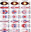 |
Fig. 2 Snapshots of three simulations for a very weak (left), a strong (middle), and a very strong (right) imposed axial dipole field. The top row shows the entropy map close to the outer boundary. The following three rows show azimuthal, latitudinal, and radial flows given in fractions of the rotation speed. The azimuthal and latitudinal magnetic fields close to the outer boundary are shown in rows 6 and 7. The last row shows the radial magnetic field at the outer boundary with the imposed dipole being subtracted. Magnetic fields are given in Gauss. Red (blue) indicates eastward, outward, or southward (westward, inward, or northward) directions. |
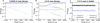 |
Fig. 3 Time evolution of the magnetic and kinetic energies during the stationary state with imposed background field (negative time) and after the background field has been switched off (positive time) for the three cases (a: 0.0025 G; b: 1.0 G, c: 2.5 G). The induced field in the 2.5 G case is stable when the background field is switched off, showing that it is generated by a subcritical dynamo. A decisive criterion for the onset of dynamo action seems that the toroidal magnetic energy exceeds the toroidal kinetic energy. Shown are the dimensionless kinetic energy, Ekin = 1/2u2, and the dimensionless magnetic energy, Emag = 1/2 (Ek/Pm) B2, integration over the simulated shell. |
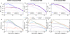 |
Fig. 4 Magnetic and kinetic energy spectra (a-c) and rms force spectra (d-f,) for the 0.025 G (a, d), 1.0 G (b, e), and 2.5 G (c, f) background dipolar field runs. The spectra of the dynamo run are very similar to the 2.5 G imposed field case. |
3.2 Light curve, hotspot offset, and dayside-to-nightside temperature difference
To obtain a model of the light curves that allows one to estimate the hotspot shift and the dayside-to-nightside temperature difference, we have to rescale from the entropy solution to temperature. For a meaningful conversion, we would need a dedicated planetary model and would have to conduct radiative transfer calculations. These results could then reveal how much each radius contributes to the phase curve observations at a given wavelength. One example of such a procedure applied to WASP-76b can be found in May et al. (2021). Since this is beyond the scope of our paper, we focus on discussing the effect of the Lorentz forces on the hotspot shifts and relative dayside-to-nightside temperature differences for a range of radii.
The stellar irradiation largely loses its impact at the depth of r = 0.945 ro, where the radiative timescale becomes comparable to the rotation timescale. Below this radius, the dynamics tends to equilibrate lateral entropy variation. Since the entropy maxima are then only mildly above the average, they would likely not contribute to any observed hotspot shift. At very shallow depths, on the other hand, the stellar irradiation clearly dominates the dynamics and the hotspot offset remains negligible, even in the hydrodynamic case without a magnetic field. We thus expect contributions to phase curve observations to originate from the region between about r = 0.96 ro and r = 0.99 ro but stress that only radial transfer modeling could reveal the true depth contribution. For illustration purposes we pick an intermediate radius of r = 0.98 ro in Figures 2 and 5.
Close to the adiabat, we can approximate variations in the specific entropy, dS , with changes in temperature,
 (37)
(37)
which suggests a rough proportionality. The irradiance variation in arbitrary units is then given by
![Mathematical equation: I(r,\theta,\varphi,t) \sim \left[\tilde{S}(r) + S(r,\theta,\varphi)\right]^4.](/articles/aa/full_html/2025/07/aa53695-25/aa53695-25-eq43.png) (38)
(38)
We modeled the visible light intensity at a certain coordinate (x, y) from an assumed radial level at a certain orbital phase, λ, using
 (39)
(39)
 (40)
(40)
 (41)
(41)
 (42)
(42)
 (43)
(43)
The light curve was then given by
 (44)
(44)
 (45)
where we integrated over one hemisphere: θ e [0, π] and
(45)
where we integrated over one hemisphere: θ e [0, π] and ![Mathematical equation: $\varphi'\in [-\pi/2,\pi/2]$](/articles/aa/full_html/2025/07/aa53695-25/aa53695-25-eq51.png) . As an example, Figure 3.2 shows the model curves, I(λ, r), for r = 0.98 ro.
. As an example, Figure 3.2 shows the model curves, I(λ, r), for r = 0.98 ro.
The phase curves are very smooth for all radii in all cases. We extracted the hotspot offset as
 (46)
(46)
The dayside and nightside equilibrium temperatures were calculated as
![Mathematical equation: T_{\rm day} (r) \sim \left[ I(\pi,r)\right]^{1/4}\;\;\mbox{and}\;\; T_{\rm night} (r) \sim \left[ I(2\pi,r)\right]^{1/4}.](/articles/aa/full_html/2025/07/aa53695-25/aa53695-25-eq53.png) (47)
(47)
We used the dayside-to-nightside temperature difference normalized with the dayside-to-nightside difference in the hydrodynamic case to quantify the impact of the magnetic field on the temperature equilibration:
 (48)
(48)
Figure 6 demonstrates that both the hotspot offset (top panel) and the dayside-to-nightside temperature difference (bottom panel) start to deviate from the pure hydrodynamic case for depths below 0.995 ro. The offset is reduced to near zero for all radii above r = 0.975 ro. Figure 2 shows that the typical eastward zonal winds are disrupted underneath the hotspot and that smaller-scale flow features start to impact the entropy pattern. Even the still rather weak radial flow may play a role since its action is amplified by the strong background entropy gradient responsible for the stable stratification.
Below r = 0.975 ro the shift becomes westward and then further decreases with depth. At r = 0.96 ro, the offset reaches about -40° for Bint = 1G and even -50° for Bint = 2.5 G. There is no global westward flow to explain the negative offsets, and radial rather than zonal flows seem to be the cause.
For Bint = 1 G (blue dots), the dayside-to-nightside temperature difference slightly increases between r = 0.965 ro and r = 0.98 ro. Below r = 0.965 ro, it strongly decreases with depth, reaching zero at about r = 0.95 ro. The magnetic effects would likely not impact the observed dayside-to-nightside temperature difference for this value of Bint. For Bint = 2.5G (green dots), however, the difference continuously decreases with depth, first slowly and then more rapidly for r < 0.97 ro. A completely equilibrated temperature is reached at about r = 0.955 ro, while for the depth likely responsible for the observations a reduction of 50% seems possible.
The retrograde hotspot shifts found for r < 0.975 ro cannot be explained by the mean zonal flow, which remains prograde around the equator at all depths. The origin seems to be advective entropy transport in latitudinal and/or radial direction by the non-axisymmetric circulation cells. Since the degree of retrograde hotspot advection at greater depth increases with the strength of the internal field, we attribute the enhancement of radial or latitudinal entropy advection to the instability-triggered Lorentz forces. A detailed analysis of the underlying nonlinear dynamics would reveal more details but is beyond the scope of this paper.
 |
Fig. 5 Total disk integrated irradiation intensity as a phase curve model at rem = 0.98ro. |
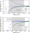 |
Fig. 6 Hotspot offset as a function of depth for the different runs (top) and dayside-to-nightside temperature difference for the magnetic cases normalized with the difference in the hydrodynamic case (bottom). The possible range of emission layers contributing to the observation is indicated in gray. |
4 Discussion
We have conducted a numerical study of the dynamics in the outer atmosphere of UHJs for the pressure range between about 1 bar and 0.01 bar. At equilibrium temperatures of around 2400 K, the effective ionization of alkali metals, combined with the fierce winds driven by one-sided irradiation, lead to large magnetic Reynolds numbers that could potentially promote strong magnetic effects. Our simulations confirm that this is indeed the case but only when the background field is strong enough to trigger a new magnetic instability.
For an imposed field with a strength below Bint = 1.0 G, the dynamics yield a complex, small-scale, quasi-stationary field, but the Lorentz force remains too weak to alter the flow. The typical prograde hostspot offset found in nonmagnetic hydrodynamic simulations, caused by a prograde zonal wind in the equatorial region, remains unchanged.
When the strength of the imposed field is raised to Bint = 1.0 G, Lorentz forces significantly impact the dynamics, promoting small-scale time-dependent disturbances that disrupt the zonal winds in the region around the substellar point. At Bint = 2.5 G, flow and magnetic field complexities increase and we can now switch out the background field without much affecting the solution. The strong imposed magnetic field has kicked off a subcritical dynamo process capable of sustaining itself.
The magnetic effects significantly reduce the hotspot offset or even cause a retrograde offset. At depths down to about r = 0.975ro, the offset is greatly diminished and nearly vanishes. At a depth of r = 0.965ro, the offset has changed from about 40° to about -20° for Bint = 1G and to about -25° for Bint = 2.5 G. Moreover, the dayside-to-nightside temperature difference drastically decreases for Bint = 2.5 G.
In terms of how this fits with observations, Table 1 shows that, of nine listed exoplanets with equilibrium temperatures above 2200 K, six exhibit a very small or retrograde hotspot shift potentially explained by the magnetic effects described here. Negative shifts would mean that the thermal emission originates from deeper rather than shallower layers. Prograde shifts are observed for KELT-1 b, WASP-33 b, and KELT-9 b. KELT-1 b’s high mass likely yields a strong degree of stable stratification, possibly suppressing the magnetic instability. WASP-33 b and KELT-9 b, with equilibrium temperatures of 2720 K and 3988 K, respectively, might experience a reduced heat flux from the planet interior, and thus a less efficient interior dynamo. To initiate the magnetic effects, the interior field would have to reach at least Bint = 1 G today. However, it would also suffice if the field had reached Bint = 2.5 Gatany time during the planet’s evolution to kick off the subcritical dynamo.
The internal field strengths assumed here align with the typical estimates for gas giants (Christensen et al. 2009; Batygin & Stevenson 2010; Yadav & Thorngren 2017). A reduced heat flux due to strong irradiation could account for a weaker field in recent times. Determining whether a planet reached Bint = 2.5 G during its lifetime requires a model of the planet’s evolution and migration, none of which is available for any exoplanet.
For an electrical conductivity of 0.5 S/m, the decisive magnetic instability sets in at Bint = 1 G and even supports a subcritical dynamo at Bint = 2.5 G. Several colder HJs also have small or retrograde hotspot offsets. At dayside equilibrium temperatures of about 1500 K, the electrical conductivity is already two orders of magnitude lower than the value assumed in our study (Dietrich et al. 2022). Since such a drastic drop cannot be compensated for by a stronger internal field, the magnetic instability would likely never set it. Other explanations are thus required to explain the retrograde offset.
We can only speculate about the type of the new magnetic instability found in our simulations. The criterion for the Taylor instability (Spruit 2002; Eq. 25 in Dietrich et al. 2022) predicts an onset at an azimuthal field strength of about Bφ = 30 G. This is already locally satisfied in our magnetic simulations for background fields starting at 0.025 G. Strong latitudinal gradients such as the ones already produced in our Bint = 0.0025 G solution further promote the Taylor instability (Eq. (A.1) in Meduri et al. 2024). However, a more detailed analysis of the instability is required to identify its character and to clarify whether there really is a connection to the Taylor instability.
Using the MHD code MagIC enabled us to study the smallscale and time-dependent instability that heavily affects the atmospheric dynamics. Such dynamics cannot be simulated with current GCMs, which have only limited capabilities for describing vertical flows and usually treat magnetic effects as a simple magnetic drag. The shallow-water models by Hindle et al. (2021a), on the other hand, concentrate on simpler largescale solutions. Other studies solving a similar set of equations to the one used here may not have encountered the instability due to the lower considered conductivities (Rogers & Komacek 2014; Rogers & Showman 2014; Rogers & McElwaine 2017; Rogers 2017). Rogers & McElwaine (2017) consider a higher conductivity on the dayside than on the nightside. Though this is arguably more realistic, we ignored this complication here. Rogers & McElwaine (2017) report that the conductivity variation promotes dynamo action. The solutions are complex and time-dependent but differ from the instability presented here.
In our simulations, we assume an electrical conductivity that is representative of the dayside. The nightside’s value may be orders of magnitude lower, meaning that the conditions for the onset of the instability may only be met on the dayside. Once initiated, the instability may nevertheless spread over the whole planet (Meduri et al. 2024), but further modeling is needed to confirm this.
Our approach has numerous limitations. The stable stratification is implemented in an ad hoc way on top of a nearly adiabatic background state. Numerical limitations necessitate an overly thick shell. The Ekman number is too large, indicating excessive viscous effects. For a better prediction of observable hotspot shifts and dayside-to-nightside temperature differences, an in-depth interior model and radiative transport simulations are needed. There is certainly room for improvement in the future.
Acknowledgements
We thank U. Christensen, J. Warnecke, and P. Wulff for discussions. VB thanks T. Bell, T. Komacek, E. May, and M. Zhang for detailed explanations of their work. This work was supported by the Deutsche Forschungsgemeinschaft (DFG) in the framework of the priority program SPP 1992 ‘Exploring the Diversity of Extrasolar Planets’. The MAGIC-code is available at an online repository (https://github.com/magic-sph/magic). This work used NumPy (Oliphant 2006; van der Walt et al. 2011), matplotlib (Hunter 2007), SciPy (Virtanen et al. 2020), and SHTns (Schaeffer 2013).
References
- Aubert, J., Gastine, T., & Fournier, A. 2017, J. Fluid Mech., 813, 558 [NASA ADS] [CrossRef] [Google Scholar]
- Batygin, K., & Stevenson, D. J. 2010, ApJ, 714, L238 [NASA ADS] [CrossRef] [Google Scholar]
- Becker, A., Bethkenhagen, M., Kellermann, C., Wicht, J., & Redmer, R. 2018, AJ, 156, 149 [Google Scholar]
- Bell, T. J., Zhang, M., Cubillos, P. E., et al. 2019, MNRAS, 489, 1995 [Google Scholar]
- Bell, T. J., Dang, L., Cowan, N. B., et al. 2021, MNRAS, 504, 3316 [NASA ADS] [CrossRef] [Google Scholar]
- Beltz, H., Rauscher, E., Roman, M. T., & Guilliat, A. 2022, AJ, 163, 35 [NASA ADS] [CrossRef] [Google Scholar]
- Cho, J. Y.-K., Polichtchouk, I., & Thrastarson, H. T. 2015, MNRAS, 454, 3423 [Google Scholar]
- Christensen, U. R., Holzwarth, V., & Reiners, A. 2009, Nature, 457, 167 [Google Scholar]
- Cowan, N. B., Agol, E., & Charbonneau, D. 2007, MNRAS, 379, 641 [NASA ADS] [CrossRef] [Google Scholar]
- Dietrich, W., & Wicht, J. 2018, Front. Earth Sci., 6, 189 [Google Scholar]
- Dietrich, W., Kumar, S., Poser, A. J., et al. 2022, MNRAS, 517, 3113 [NASA ADS] [CrossRef] [Google Scholar]
- Dobbs-Dixon, I., & Agol, E. 2013, MNRAS, 435, 3159 [NASA ADS] [CrossRef] [Google Scholar]
- Dobbs-Dixon, I., & Lin, D. N. C. 2008, ApJ, 673, 513 [NASA ADS] [CrossRef] [Google Scholar]
- French, M., Becker, A., Lorenzen, W., et al. 2012, ApJS, 202, 5 [NASA ADS] [CrossRef] [Google Scholar]
- Gastine, T., & Wicht, J. 2021, Icarus, 368, 114514 [NASA ADS] [CrossRef] [Google Scholar]
- Harrington, J., Hansen, B. M., Luszcz, S. H., et al. 2006, Science, 314, 623 [NASA ADS] [CrossRef] [Google Scholar]
- Heng, K., Menou, K., & Phillipps, P. J. 2011, MNRAS, 413, 2380 [NASA ADS] [CrossRef] [Google Scholar]
- Hindle, A. W., Bushby, P. J., & Rogers, T. M. 2019, ApJ, 872, L27 [NASA ADS] [CrossRef] [Google Scholar]
- Hindle, A. W., Bushby, P. J., & Rogers, T. M. 2021a, ApJ, 922, 176 [CrossRef] [Google Scholar]
- Hindle, A. W., Bushby, P. J., & Rogers, T. M. 2021b, ApJ, 916, L8 [NASA ADS] [CrossRef] [Google Scholar]
- Hunter, J. D. 2007, Comput. Sci. Eng., 9, 90 [NASA ADS] [CrossRef] [Google Scholar]
- Iro, N., Bézard, B., & Guillot, T. 2005, A&A, 436, 719 [NASA ADS] [CrossRef] [EDP Sciences] [Google Scholar]
- Jones, C. A., Boronski, P., Brun, A. S., et al. 2011, Icarus, 216, 120 [NASA ADS] [CrossRef] [Google Scholar]
- Knutson, H. A., Charbonneau, D., Allen, L. E., et al. 2007, Nature, 447, 183 [NASA ADS] [CrossRef] [Google Scholar]
- Kumar, S., Poser, A. J., Schöttler, M., et al. 2021, Phys. Rev. E, 103, 063203 [Google Scholar]
- Lago, R., Gastine, T., Dannert, T., Rampp, M., & Wicht, J. 2021, Geosci. Model Dev., 14, 7477 [NASA ADS] [CrossRef] [Google Scholar]
- May, E. M., Komacek, T. D., Stevenson, K. B., et al. 2021, AJ, 162, 158 [NASA ADS] [CrossRef] [Google Scholar]
- May, E. M., Stevenson, K. B., Bean, J. L., et al. 2022, AJ, 163, 256 [NASA ADS] [CrossRef] [Google Scholar]
- Meduri, D. G., Jouve, L., & Lignières, F. 2024, A&A, 683, A12 [NASA ADS] [CrossRef] [EDP Sciences] [Google Scholar]
- Oliphant, T. E. 2006, A Guide to NumPy, 1 (Trelgol Publishing USA) [Google Scholar]
- Parmentier, V., & Crossfield, I. J. M. 2018, in Handbook of Exoplanets, eds. H.-J. Deeg & J. A. Belmonte, Springer eBook Collection (Cham: Springer), 1419 [Google Scholar]
- Perna, R., Menou, K., & Rauscher, E. 2010, ApJ, 719, 1421 [NASA ADS] [CrossRef] [Google Scholar]
- Parmentier, V., Fortney, J. J., Showman, A. P., Morley, C., & Marley, M. S. 2016, ApJ, 828, 22 [Google Scholar]
- Rauscher, E., & Menou, K. 2012, ApJ, 745, 78 [Google Scholar]
- Rauscher, E., & Menou, K. 2013, ApJ, 764, 103 [NASA ADS] [CrossRef] [Google Scholar]
- Rauscher, E., & Kempton, E. M. R. 2014, ApJ, 790, 79 [NASA ADS] [CrossRef] [Google Scholar]
- Rogers, T. M. 2017, Nat. Astron., 1, 0131 [Google Scholar]
- Rogers, T. M., & Komacek, T. D. 2014, ApJ, 794, 132 [NASA ADS] [CrossRef] [Google Scholar]
- Rogers, T. M., & McElwaine, J. N. 2017, ApJ, 841, L26 [Google Scholar]
- Rogers, T. M., & Showman, A. P. 2014, ApJ, 782, L4 [NASA ADS] [CrossRef] [Google Scholar]
- Roman, M., & Rauscher, E. 2017, ApJ, 850, 17 [NASA ADS] [CrossRef] [Google Scholar]
- Schaeffer, N. 2013, Geochem. Geophys. Geosyst., 14, 751 [NASA ADS] [CrossRef] [Google Scholar]
- Schwaiger, T., Gastine, T., & Aubert, J. 2019, Geophys. J. Roy. Astron. Soc., 219, S101 [Google Scholar]
- Showman, A. P., & Guillot, T. 2002, A&A, 385, 166 [NASA ADS] [CrossRef] [EDP Sciences] [Google Scholar]
- Showman, A. P., & Polvani, L. M. 2011, ApJ, 738, 71 [Google Scholar]
- Showman, A. P., Tan, X., & Parmentier, V. 2020, Space Sci. Rev., 216, 139 [Google Scholar]
- Snellen, I. A. G., de Kok, R. J., de Mooij, E. J. W., & Albrecht, S. 2010, Nature, 465, 1049 [Google Scholar]
- Spruit, H. C. 2002, A&A, 381, 923 [CrossRef] [EDP Sciences] [Google Scholar]
- van der Walt, S., Colbert, S. C., & Varoquaux, G. 2011, Comput. Sci. Eng., 13, 22 [Google Scholar]
- Virtanen, P., Gommers, R., Oliphant, T. E., et al. 2020, Nat. Methods, 17, 261 [Google Scholar]
- Wicht, J. 2002, Phys. Earth Planet. Interiors, 132, 281 [CrossRef] [Google Scholar]
- Wicht, J., Gastine, T., Duarte, L. D. V., & Dietrich, W. 2019, A&A, 629, A125 [NASA ADS] [CrossRef] [EDP Sciences] [Google Scholar]
- Wulff, P. N. 2023, PhD thesis, Georg-August-Universitat Gottingen, Germany [Google Scholar]
- Wulff, P. N., Dietrich, W., Christensen, U. R., & Wicht, J. 2022, MNRAS, 517, 5584 [Google Scholar]
- Yadav, R. K., & Thorngren, D. P. 2017, ApJ, 849, L12 [NASA ADS] [CrossRef] [Google Scholar]
All Tables
All Figures
|
Fig. 1 Dimensionless equilibrium entropy pattern, Seq, used to model the stellar irradiation in the Newtonian cooling scheme (see Equations (20) and (21)). |
| In the text | |
|
Fig. 2 Snapshots of three simulations for a very weak (left), a strong (middle), and a very strong (right) imposed axial dipole field. The top row shows the entropy map close to the outer boundary. The following three rows show azimuthal, latitudinal, and radial flows given in fractions of the rotation speed. The azimuthal and latitudinal magnetic fields close to the outer boundary are shown in rows 6 and 7. The last row shows the radial magnetic field at the outer boundary with the imposed dipole being subtracted. Magnetic fields are given in Gauss. Red (blue) indicates eastward, outward, or southward (westward, inward, or northward) directions. |
| In the text | |
|
Fig. 3 Time evolution of the magnetic and kinetic energies during the stationary state with imposed background field (negative time) and after the background field has been switched off (positive time) for the three cases (a: 0.0025 G; b: 1.0 G, c: 2.5 G). The induced field in the 2.5 G case is stable when the background field is switched off, showing that it is generated by a subcritical dynamo. A decisive criterion for the onset of dynamo action seems that the toroidal magnetic energy exceeds the toroidal kinetic energy. Shown are the dimensionless kinetic energy, Ekin = 1/2u2, and the dimensionless magnetic energy, Emag = 1/2 (Ek/Pm) B2, integration over the simulated shell. |
| In the text | |
|
Fig. 4 Magnetic and kinetic energy spectra (a-c) and rms force spectra (d-f,) for the 0.025 G (a, d), 1.0 G (b, e), and 2.5 G (c, f) background dipolar field runs. The spectra of the dynamo run are very similar to the 2.5 G imposed field case. |
| In the text | |
|
Fig. 5 Total disk integrated irradiation intensity as a phase curve model at rem = 0.98ro. |
| In the text | |
|
Fig. 6 Hotspot offset as a function of depth for the different runs (top) and dayside-to-nightside temperature difference for the magnetic cases normalized with the difference in the hydrodynamic case (bottom). The possible range of emission layers contributing to the observation is indicated in gray. |
| In the text | |
Current usage metrics show cumulative count of Article Views (full-text article views including HTML views, PDF and ePub downloads, according to the available data) and Abstracts Views on Vision4Press platform.
Data correspond to usage on the plateform after 2015. The current usage metrics is available 48-96 hours after online publication and is updated daily on week days.
Initial download of the metrics may take a while.