| Issue |
A&A
Volume 694, February 2025
|
|
|---|---|---|
| Article Number | A53 | |
| Number of page(s) | 25 | |
| Section | Planets, planetary systems, and small bodies | |
| DOI | https://doi.org/10.1051/0004-6361/202453019 | |
| Published online | 03 February 2025 | |
Anisotropic tidal dissipation in misaligned planetary systems
IMCCE, Observatoire de Paris, Université PSL, CNRS, Sorbonne Université,
77 Avenue Denfert-Rochereau,
Paris
75014,
France
★ Corresponding author; pierre.auclair-desrotour@obspm.fr
Received:
15
November
2024
Accepted:
16
December
2024
Context. Tides are the main driving force behind the long-term evolution of planetary systems. The associated energy dissipation and momentum exchanges are commonly described by Love numbers, which relate the exciting potential to the tidally perturbed potential. These transfer functions are generally assumed to depend solely on tidal frequency and body rheology, following the isotropic assumption, which presumes invariance of properties by rotation about the centre of mass.
Aims. We examine the limitations of the isotropic assumption for fluid bodies, in which Coriolis acceleration breaks spherical symmetry, resulting in rotational scattering and complex tidal responses.
Methods. Using angular momentum theory, we derived a new formalism to calculate the tidal rates of energy and momentum transfers in non-isotropic cases. We applied this formalism to the Earth-Moon system to assess the effects of anisotropy in planet-satellite systems with misaligned spin and orbital angular momenta.
Results. Our findings indicate that the isotropic assumption can introduce significant errors in planetary evolution models, particularly in the dynamical tide regime. These errors stem from forced wave resonances, with inaccuracies in energy dissipation scaling in proportion to resonance amplification factors.
Key words: Earth / planets and satellites: dynamical evolution and stability / planets and satellites: oceans / planets and satellites: terrestrial planets / planet-star interactions
© The Authors 2025
 Open Access article, published by EDP Sciences, under the terms of the Creative Commons Attribution License (https://creativecommons.org/licenses/by/4.0), which permits unrestricted use, distribution, and reproduction in any medium, provided the original work is properly cited.
This article is published in open access under the Subscribe to Open model. Subscribe to A&A to support open access publication.
1 Introduction
Tides are among the most fundamental mechanisms driving long-term celestial dynamics. They originate from the differential gravitational forces exerted by orbiting bodies on one another, leading to mass redistribution and energy dissipation. This process induces the transfer of angular momentum and energy between the spin of celestial bodies and their orbits, resulting in internal heating and progressive evolution of planetary systems over extensive timescales (e.g. Ogilvie 2014). In particular, tides shape the system architecture by establishing stable equilibrium states. The main stabilising effects include (i) circularisation, which tends to make orbits circular; (ii) synchronisation, whereby orbital and rotational periods become equal to each other; and (iii) alignment, whereby equatorial and orbital planes converge (e.g. Hut 1980, 1981).
Tidal dissipation also impacts the climate and surface conditions of rocky planets by influencing their capacity to maintain liquid water on their surfaces (see e.g. Bolmont 2018, and references therein). The associated tidal heating can transform the thermal state of such bodies, potentially melting interiors and triggering volcanism, as was seen on Io (Peale et al. 1979; Peale 2003). Similarly, Tyler (2008) showed that tides can produce substantial heat fluxes on icy moons in the outer Solar System, and thus sustain long-lived sub-surface oceans of liquid water (see also Tyler 2009, 2011, 2014, 2020). The dissipative processes generating tidal heating and the interplay between the oceanic response and the upper icy crust were subsequently examined by several authors (e.g. Matsuyama 2014; Kamata et al. 2015; Beuthe 2016; Matsuyama et al. 2018; Hay & Matsuyama 2019; Rekier et al. 2019; Rovira-Navarro et al. 2023).
Finally, tidal interactions are crucial to understanding the Earth-Moon system’s 4.5-billion-year climato-biologic evolution, especially through their effects on Earth’s length of day (LOD) and obliquity (e.g. Daher et al. 2021; Tyler 2021; Farhat et al. 2022a). On Earth, ocean tides dominate, accounting for over 90% of energy dissipation (e.g. Egbert & Ray 2000, 2001). As was proposed by Zahnle & Walker (1987), atmospheric thermal tides – namely, tides caused by Solar radiative flux – may have equally played an important role by partly counteracting the decelerating effect of gravitational tides on Earth’s rotation during the Precambrian. However, despite sparse geological data suggesting that Earth’s mid-Proterozoic LOD was stabilised (Bartlett & Stevenson 2016; Mitchell & Kirscher 2023; Wu et al. 2023), tidal locking likely never occurred (Farhat et al. 2024; Laskar et al. 2024), unlike on Venus, which is maintained in asynchronous rotation by thermal tides (Gold & Soter 1969; Ingersoll & Dobrovolskis 1978; Correia & Laskar 2001, 2003; Leconte et al. 2015).
Tides are usually considered as small perturbations around an equilibrium state, allowing for a linearised approach (e.g. Mathis et al. 2013). The linear response of a body to tidal forces is quantified by the potential Love number, named after A.E.H. Love, which relates the perturbed gravitational potential – resulting from variations in self-attraction – to the tide-raising potential (e.g. Ogilvie 2014). This potential Love number is a complex-valued, dimensionless transfer function that varies with tidal frequency and accounts for both tidal deformation and energy dissipation in the frequency domain1. Commonly denoted by  , where l and m represent the degree and order of the spherical harmonic, respectively, the Love number is often simplified to a single parameter, k2, or the degree-2 Love number, which depends solely on the tidal frequency and the internal physics of the tidally perturbed body (e.g. Mathis et al. 2013; Correia & Valente 2022; Valente & Correia 2022). Such an approximation implies rotational invariance around the body’s centre of mass, meaning that the background fields and tidal dynamics equations are independent of the body’s orientation relative to the perturber’s orbit. Throughout this study, we refer to this simplification as the ‘isotropic assumption’, noting that isotropy designates uniformity in all orientations. Although alternative terminology can be used, we opt for this one because it evokes a meaningful analogy between tidal perturbations and light rays propagating through an optical medium.
In solid bodies, the isotropic assumption is generally reasonable as a first-order approximation, since their internal structure and visco-elastic properties are primarily determined by radial self-attraction and pressure forces (e.g. Sotin et al. 2007). The resulting bodily tide is essentially a quasi-static adjustment to tidal forces, without inertial effects2. Consequently, all tidal constituents are straightforwardly obtained from the equatorial degree-2 Love number describing the semidiurnal tidal bulge in the coplanar-circular configuration, which is just evaluated across several tidal frequencies – one per constituent. As a corollary, the degree-2 Love number is a symmetric function of the tidal frequency, with an even real part and an odd imaginary part, as was discussed by Efroimsky (2012a).
Unlike solid bodies, fluid layers exhibit anisotropic tidal responses – even in spherically symmetric cases – because fluid particle motion is influenced by Coriolis acceleration. By introducing a preferred direction (the spin axis), Coriolis acceleration distorts tidal flows, making the fluid response markedly different from that of solid materials. Notably, anisotropy induces scattering: the spherical harmonics coefficients describing the fluid tidal response are energetically coupled together instead of being independent as in solid bodies. This symmetry-breaking effect is intensified by the so-called dynamical tide – the component of the response associated with wave propagation (Zahn 1975) – since each oscillatory fluid mode can resonate at a specific frequency (e.g. Longuet-Higgins 1968; Savonije & Witte 2002; Ogilvie & Lin 2004; Ogilvie 2013, 2014; Auclair-Desrotour et al. 2018).
A wide variety of wave types can arise, mixing or remaining distinct depending on the fluid layer’s properties (e.g. Fuller et al. 2024). For instance, ocean tides on rocky planets are predominantly governed by long-wavelength surface gravity modes (Longuet-Higgins 1968; Cartwright 1977). These waves, restored by self-attraction, resemble the planetary-scale compressibility modes known as Lamb waves (e.g. Bretherton 1969; Lindzen & Blake 1972) that can be gravitationally or radiatively driven in planetary atmospheres, including Earth’s (e.g. Farhat et al. 2024). In other cases, the dynamical tide may consist of inertial, gravity, Alfvén, or acoustic waves, each restored by different forces – Coriolis acceleration, buoyancy (in stably stratified layers), magnetic tension, or pressure, respectively (e.g. Mathis et al. 2013; Rieutord 2015) – as is observed in stars and the fluid envelopes of giant planets.
Tidal anisotropy is further amplified by complex geometries. On Earth, continental coastlines redirect tidal flows, shifting resonant frequencies and disrupting symmetries (e.g. Green et al. 2017; Blackledge et al. 2020; Lyard et al. 2021; Auclair- Desrotour et al. 2023), while shallow seas add dynamic coupling effects between shelf and ocean tides (e.g. Brian K. Arbic & Garrett 2009; Arbic & Garrett 2010; Wilmes et al. 2023). Owing to these complexities, the role of anisotropic effects in planetary system evolution remains poorly understood. Yet, these effects may significantly alter the characteristic signatures of the dynamical tide, which manifests as staircase-like variations in orbital parameters during resonance episodes (e.g. Auclair- Desrotour et al. 2014; Tyler 2021; Motoyama et al. 2020; Farhat et al. 2022a; Huang et al. 2024; Zhou et al. 2024; Wu et al. 2024).
In the present study, we examine the limitations of the isotropic approximation to characterise their impact on the modelled orbital evolution of binary systems with misaligned spin and orbital angular momenta. Our approach extends previous research on the past history of the Earth-Moon system (Farhat et al. 2022a,b, 2024; Auclair-Desrotour et al. 2023). In Sect. 2, building on insights from Ogilvie (2013) and Boué (2017), we introduce a new formalism to calculate the time-averaged tidal rates of angular momentum and energy transfers in non-isotropic configurations. We further complement this formalism in Sect. 3 with the equations governing the long-term tidal evolution of a planet-perturber system. Finally, in Sect. 4, we apply these methods to an idealised Earth-Moon system, which allows us to probe the validity domain of the isotropic assumption and quantify related errors. Our findings reveal that the isotropic assumption results in notably inaccurate predictions for evolution models in the dynamical tide regime of fluid bodies, with errors scaling proportionally to the amplification factors associated with resonantly excited tidal waves. Notations and acronyms used throughout this paper are listed in the nomenclature in Appendix A.
2 Tidal torque and tidally dissipated power
2.1 Tidal torque as a function of tidal potentials
In this work, we examine the tidal interaction of two bodies orbiting around their centre of mass. For simplicity, we assume the central body to be a planet of mass Mp and radius Rp, and the tidal perturber a satellite of mass Ms. Nevertheless, the derivations presented in this section apply to any combination of central bodies and perturbers. The satellite induces a tidal potential, UT, which disturbs the planet’s mass distribution. This, in turn, generates a deformation potential, UD, which influences the system’s orbital evolution. Our initial aim is to establish the relationship between these two gravitational potentials and the rates of angular momentum and energy exchanges between the planet and satellite. These derivations are framed within linear theory, in which tides are treated as infinitesimal perturbations, and will later be used in Sect. 3 for numerical calculations.
We adopt a non-rotating, geocentric frame of reference, 𝓡f: (O, ex, ey, ez), centred at the planet’s centre of mass, O. The corresponding Cartesian unit vectors, (ex, ey, ez), point towards distant stars. In 𝓡f, the position of any point M is described using spherical polar coordinates (r, θ, φ), where r is the radial distance, θ the colatitude, and φ the longitude. The position vector of point M is denoted as r ≡ rer, while the position vector of the satellite’s centre of mass is given by rs = rser, where er is the unit radial vector. Additionally, we define the rotating reference frame associated with the planet, 𝓡: (O, eX, eY, eZ), where eZ aligns with the planet’s spin axis and points towards the north pole, while the other two unit vectors, eX and eY, define orthogonal directions in the planet’s equatorial plane. In this rotating frame, the position of a point is described by the spherical coordinates  .
.
As is illustrated by Fig. 1, the transformation between the two frames, 𝓡f : (O, ex, ey, ez) → 𝓡: (O, eX, eY, eZ), is represented by the 3-2-3 Euler rotation matrix R (α,β, γ) = R3 (α) R2 (β) R3 (γ), where R2 and R3 are the rotation matrices around the second and the third axes, respectively. The matrix R is parametrised by the Euler angles (α, β, γ) given by (e.g. Varshalovich et al. 1988, Eq. (54) p. 30)
![$R(\alpha ,\beta ,\gamma ) \equiv \left[ {\matrix{ {{C_\alpha }{C_\beta }{C_\gamma } - {S_\alpha }{S_\gamma }} & { - {C_\alpha }{C_\beta }{S_\gamma } - {S_\alpha }{C_\gamma }} & {{C_\alpha }{S_\beta }} \cr {{S_\alpha }{C_\beta }{C_\gamma } + {C_\alpha }{S_\gamma }} & { - {S_\alpha }{C_\beta }{S_\gamma } + {C_\alpha }{C_\gamma }} & {{S_\alpha }{S_\beta }} \cr { - {S_\beta }{C_\gamma }} & {{S_\beta }{S_\gamma }} & {{C_\beta }} \cr } } \right],$](/articles/aa/full_html/2025/02/aa53019-24/aa53019-24-eq3.png) (1)
(1)
with Cϕ = cos ϕ and Sϕ = sin ϕ for ϕ = α, β, or γ. Here, α and β denote the planet’s precession and nutation angles, respectively, while γ represents the intrinsic rotation angle. In Kaula’s theory, the angles α and β evolve over timescales that are much longer than typical tidal oscillation periods (e.g. Efroimsky & Williams 2009). Therefore, they are treated as constants in the formulation of the tidal problem. This is not the case for the intrinsic rotation angle, γ, which describes the planet’s spin, and explicitly varies with time, t, as
 (2)
(2)
where Ω is the planet’s spin angular velocity.
The torque exerted by a force, F, about the origin point, O, on a planet occupying a volume, 𝒱, is expressed in spherical coordinates (r, θ, φ) as
 (3)
(3)
where dV is an infinitesimal volume element, ρ is the local density, and × denotes the cross product. Following the convention of Zahn (1966), the tidal force is expressed as
 (4)
(4)
where ∇ designates the gradient operator (see Appendix B). The tide-raising potential is given by (e.g. Kaula 1964; Efroimsky & Williams 2009)
 (5)
(5)
with G = 6.67430 × 10⁻¹¹ m3 kg−1 s−2 being the universal gravitational constant (Tiesinga et al. 2021).
Since tidal oscillation periods are typically much shorter than the characteristic evolution timescales of the orbital system, we focus exclusively on the time-averaged tidal effects on the planet and satellite’s motions. We denote by 〈 f 〉 the average of any function of time, f, defined as
 (6)
(6)
The time-averaged tidal torque exerted about the three directions of the Galilean frame (Rf ) is thus given by
 (7)
(7)
where 𝓛 ≡ r × ∇ is the angular momentum operator (Varshalovich et al. 1988, Sect. 2.2), and δρ is the local tidal density variation. We can express δρ in terms of the gravitational potential of the tidally distorted body, UD, using Poisson’s equation (e.g. Arfken & Weber 2005, Sect. 1.14),
 (8)
(8)
with ∇2 denoting the Laplacian operator, which leads to
 (9)
(9)
It is important to note that both UT and UD are expressed in the system of coordinates associated with the non-rotating frame of reference (𝓡f), specifically (r, θ, φ).
Ogilvie (2013) demonstrated that the integral in Eq. (9) can, in fact, be carried out over any volume including the tidally distorted body. We therefore considered a simply connected domain, 𝒱∗, which includes the planet but not the perturber, as is illustrated by Fig. 2, and we introduced the vector, A = (Ax, Ay, Az), defined as
 (10)
(10)
Since 𝒱* excludes the perturber, we have ∇2UT = 0 in 𝒱*. Furthermore, the angular momentum and Laplacian operators can be interchanged (e.g. Varshalovich et al. 1988, Sect. 2.2.2.), giving
 (11)
(11)
As a result, the integral in Eq. (10) is rewritten as
![$A = \mathop \smallint \limits_{{{\cal V}_*}} \left[ {{\cal L}{U_{\rm{T}}}{\nabla ^2}{U_{\rm{D}}} - {U_{\rm{D}}}{\nabla ^2}\left( {{\cal L}{U_{\rm{T}}}} \right)} \right]{\rm{d}}V.$](/articles/aa/full_html/2025/02/aa53019-24/aa53019-24-eq14.png) (12)
(12)
Thus, by virtue of Green’s second identity (e.g. Arfken & Weber 2005, Sect. 1.11), any component, Av, of A, where v = x,y or z, is expressed as
![${A_v} = \mathop \oint \limits_{\partial {{\cal V}_*}} \left[ {\left( {{{\cal L}_v}{U_{\rm{T}}}} \right)\nabla {U_{\rm{D}}} - {U_{\rm{D}}}\nabla \left( {{{\cal L}_v}{U_{\rm{T}}}} \right)} \right] \cdot {\rm{d}}S.$](/articles/aa/full_html/2025/02/aa53019-24/aa53019-24-eq15.png) (13)
(13)
Here, dS is an outward-pointing infinitesimal surface element vector, and ∂𝒱∗ is the boundary of 𝒱∗. This allows the time- averaged torques exerted about the x, y, and z axes of 𝓡f to be written as
![${{\cal T}_x} = - {1 \over {4\pi G}}\langle \mathop \oint \limits_{\partial {{\cal V}_*}} \left[ {\left( {{{\cal L}_x}{U_{\rm{T}}}} \right)\nabla {U_{\rm{D}}} - {U_{\rm{D}}}\nabla \left( {{{\cal L}_x}{U_{\rm{T}}}} \right)} \right] \cdot {\rm{d}}S\rangle ,$](/articles/aa/full_html/2025/02/aa53019-24/aa53019-24-eq16.png) (14)
(14)
![${{\cal T}_y} = - {1 \over {4\pi G}}\langle \mathop \oint \limits_{\partial {{\cal V}_*}} \left[ {\left( {{{\cal L}_y}{U_{\rm{T}}}} \right)\nabla {U_{\rm{D}}} - {U_{\rm{D}}}\nabla \left( {{{\cal L}_y}{U_{\rm{T}}}} \right)} \right] \cdot {\rm{d}}S\rangle ,$](/articles/aa/full_html/2025/02/aa53019-24/aa53019-24-eq17.png) (15)
(15)
![${{\cal T}_} = - {1 \over {4\pi G}}\langle \mathop \oint \limits_{\partial {{\cal V}_*}} \left[ {\left( {{{\cal L}_}{U_{\rm{T}}}} \right)\nabla {U_{\rm{D}}} - {U_{\rm{D}}}\nabla \left( {{{\cal L}_}{U_{\rm{T}}}} \right)} \right] \cdot {\rm{d}}S\rangle .$](/articles/aa/full_html/2025/02/aa53019-24/aa53019-24-eq18.png) (16)
(16)
Finally, the rate of energy transferred from the perturber’s orbital motion to the planet’s rotation is the time-averaged tidal power, 𝒫T, which we express as a function of both the forcing and deformation tidal potentials too (e.g. Auclair-Desrotour et al. 2023),
 (17)
(17)
By invoking Green’s second identity once again, we rewrite this expression as
![${_{\rm{T}}} = - {1 \over {4\pi G}}\langle \mathop {\mathop \oint \nolimits^ }\limits_{\partial {{\cal V}_*}} \left[ {{U_{\rm{T}}}\nabla \left( {{\partial _t}{U_{\rm{D}}}} \right) - \left( {{\partial _t}{U_{\rm{D}}}} \right)\nabla {U_{\rm{T}}}} \right] \cdot {\rm{d}}S\rangle .$](/articles/aa/full_html/2025/02/aa53019-24/aa53019-24-eq20.png) (18)
(18)
The time-averaged tidally dissipated power, 𝒫diss, can be readily deduced from 𝒯 and 𝒫T, as was demonstrated by Ogilvie (2013) and as is discussed in Sect. 3.2. Since Eqs. (14–16) and Eq. (18) provide the rates of momentum and energy exchanges as functions of the tide-raising and deformation gravitational potentials, UT and UD, we shall specify these two potentials in the following.
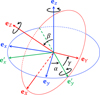 |
Fig. 1 Euler angles (α, β, γ) corresponding to the 3-2-3 Euler rotation matrix defined by Eq. (1), which describes the change of coordinate systems 𝓡f : O, ex, ey, ez → 𝓡: (O, eX, eY, eZ). |
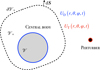 |
Fig. 2 Diagram illustrating the domain 𝒱∗, which includes the central body while excluding the perturber. |
2.2 Tidal gravitational potential of the distorted planet
In linear theory, the tidal forcing and deformation potentials in Eqs. (14–16) and Eq. (18) are both series of periodic functions of time, since UT is composed of oscillatory components. Consequently, it is appropriate to transition from the temporal to the frequency domain by expanding both potentials in Fourier series. These manipulations yield
 (19)
(19)
 (20)
(20)
where ℜ denotes the real part of a complex number (with ℑ referring to the imaginary part), i represents the imaginary unit (i2 = −1), σk is the k-th forcing tidal frequency, σk,q,p is the frequency of the tidal response defined by the triplet (k, q, p),
 (21)
(21)
and  and
and  designate the corresponding complex distributions for each potential. The frequencies, σk, are expressed as
 (22)
(22)
where ns is the anomalistic mean motion of the perturber in the Galilean frame, and the integer, k, ranges from 0 to +∞3. It is noteworthy that the summations over q and p in Eqs. (19) and (20) result from the forward and backward rotations between the Galilean and rotating frames of reference, as will be discussed further.
Outside the planet, the coefficients,  and
and  , are expressed as series of spherical harmonics,
  , of degree l and order m, as follows:
 (23)
(23)
 (24)
(24)
where  and
and  are complex weighting coefficients associated with the triplet (k, l, m) and the quintuplet (k, l, m, p, q), respectively. The spherical harmonics,
  , in Eqs. (23) and (24) are explicitly defined in Appendix D.
The gravitational potential induced by the planet’s tidal response is usually obtained in the rotating frame of reference (𝓡), where the equations governing the planet’s tidal response are straightforwardly formulated. This requires expressing the tidal components given by Eqs. (23) and (24) as functions of the coordinates associated with 𝓡, namely  . This step is easily completed by considering the rotation operator of spherical harmonics: the spherical harmonics sharing the same degree in the Galilean and rotated systems of coordinates are linked through the relations (Varshalovich et al. 1988, Sect. 4.1)
 (25)
(25)
 (26)
(26)
In the above equations, the notation  refers to the Wigner D- functions (Varshalovich et al. 1988, Sect. 4.3, Eq. (1)), which are detailed in Appendix E, and
  denotes the complex conjugate of
  . Besides, we recall that γ is a function of time, as is defined in Eq. (2).
Using Eq. (25) in Eq. (23), we express the tideraising potential in the coordinates of the rotating frame of reference,
 (27)
(27)
where the integer k runs from 0 to +∞ and q from −∞ to +∞. In this expression, the tidal frequencies,  , are defined as
 (28)
(28)
and the complex weighting coefficients,  , as
, as
 (29)
(29)
The component of the forcing associated with the triplet (l, q, k) generates a tidal gravitational potential oscillating with the same frequency, but not necessarily with the same spatial distribution. The spatially dependent factor of this potential is expressed in general as
 (30)
(30)
with  being the transfer function associated with the harmonic of degree s and order p. It is noteworthy that
  stands for a generalised Love number accounting for the fact that the spatial dependence of the tidal response generally differs from that of the tide-raising potential because of rotational scattering. For spherically isotropic bodies, this transfer function simplifies to
  , where δq,p designates the Kronecker delta function, such that δq,p = 1 if q = p and δq,p = 0 otherwise.
In the coordinates of the rotating frame,, the gravitational potential of the tidally distorted body can be expressed as
 (31)
(31)
where the spatial distributions associated with the frequencies,  , are given by
 (32)
(32)
In this expression, the complex weighting coefficients,  , are defined as
 (33)
(33)
By changing the coordinates from  to (r, θ, φ), we obtain the gravitational potential components
  , introduced in Eq. (24), first as functions of the
  coefficients,
 (34)
(34)
and second, using Eq. (33), in terms of the  ,
,
 (35)
(35)
Finally, substituting Eq. (29) into the above equation, we rewrite  as a function of the weighting coefficients of the forcing tidal potential in the inertial frame, 𝓡f,
 (36)
(36)
This formulation of the deformation potential accounts for the possible coupling of spherical modes in the tidal response. When the central body is assumed to be spherically isotropic, no such coupling occurs. In that case, each component of the response corresponds to the same spherical harmonic as the forcing component generating it. Therefore, the summation over s in Eq. (36) vanishes and  simplifies to
 (37)
(37)
2.3 Components of the tidal torque
As a final step, we express the tidal torque and tidally dissipated power, derived in Eqs. (14–16) and Eq. (18), in terms of the complex coefficients from the multipole expansions of the forcing and deformation tidal potential. These are the coefficients  and
and  introduced in Eqs. (23) and (24), respectively. This step is not straightforward, as the angular momentum operator introduces significant mathematical complexities. However, these difficulties can be elegantly addressed using angular momentum theory, as is demonstrated by Boué (2017). In this approach inspired from quantum mechanics, the problem is simplified by changing to a system of coordinates in which the action of the angular momentum operator on spherical harmonics is easily formulated. The terms involving the angular momentum operator in Eqs. (14–16) and Eq. (18) are then directly obtained by converting back to the Cartesian system, (x, y, z).
Following Boué (2017), we introduced the set of complex unit vectors (e+, e0, e−), where the coordinates of any vector, a, are represented as (a+, a0, a−). These are related to the Cartesian coordinates (ax, ay, az} in the reference frame, 𝓡f, by
 (38)
(38)
For v ∈ {−, 0, +} (i.e. v = −1,0,1, respectively), the v component, 𝓛ν, of the angular momentum operator applied to a spherical harmonic,  , is expressed as
 (39)
(39)
where the coefficients,  are real and defined as (Varshalovich et al. 1988)
 (40)
(40)
The forcing and deformation tidal potentials, UT and UD, are written in terms of the complex potentials, ŨT and ŨD, as follows:
 (41)
(41)
Since the real part and angular momentum operator can be interchanged, we have
 (42)
(42)
Using the change of coordinates introduced in Eq. (38), we obtain
 (43)
(43)
 (44)
(44)
 (45)
(45)
To express the torques defined in Eqs. (14–16) in terms of the Fourier components of ŨT and ŨD, one must compute the conju- gates of 𝓛xŨT, 𝓛yŨT, and 𝓛zŨT, as well as the radial component of their gradients and of the gradient of ŨD. The quantity, 𝓛v ŨT, is given by
 (46)
(46)
This results in
 (47)
(47)
 (48)
(48)
 (49)
(49)
with k ranging from 0 to +∞ and v = ±1.
Similarly, the radial component of the gradient of ŨD is given by
 (50)
(50)
where k runs from 0 to +∞, and q and p from −∞ to +∞. However, only the components associated with the frequencies σk of the forcing tidal potential contribute to the tidal torque. These correspond to terms where p = q. Thus, the gradient of the tidal potential is rewritten as
 (51)
(51)
where 𝒰 represents the component of ŨD that does not generate any torque in average.
The time-averaged components of the torque can be straightforwardly deduced from the preceding derivations. In essence, we consider the function f defined as
 (52)
(52)
where 𝒱 denotes the spatial domain over which the integral is evaluated, dV represents an infinitesimal volume element, and A and B are two functions expressed as
 (53)
(53)
 (54)
(54)
In the above equations, the complex functions, A and B, are sinusoidal time-oscillating functions of positive frequencies, σ1 and σ2, respectively, multiplied by complex spatial distributions,
 (55)
(55)
 (56)
(56)
As is demonstrated in Appendix C, the time-averaged value of f, defined by Eq. (6), can be expressed in terms of the complex spatial distributions Ã0 and  as
as
 (57)
(57)
By applying this identity to the components of the tidal torque (Eqs. (14–16)) and tidal power (Eq. (18)), and following the steps detailed in Appendix F, we arrive at
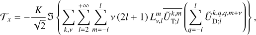 (58)
(58)
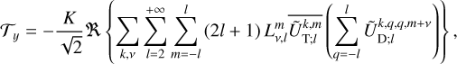 (59)
(59)
 (60)
(60)
 (61)
(61)
where k runs from 0 to +∞, ν = ±1, and K is a constant defined as
 (62)
(62)
The formulae given by Eqs. (58–61) enable the calculation of the average rates of angular momentum and energy transfer in a general setting. Notably, these formulae remain valid even if the system does not conform to the spherical isotropy assumptions that typically prevail in the linear theory of bodily tides (see e.g. Efroimsky & Williams 2009, Sect. 4) or in the equilibrium tide model. Specifically, (i) the energy dissipation rate of one component is not solely dependent on the associated tidal frequency within this framework, and (ii) the deformation of the planet’s shape can differ spatially from the tide-generating potential, though it remains linearly related to it.
3 Dynamics of a planet-satellite system
3.1 Tide-raising gravitational potential
The tidal torque and power, as is expressed in Eqs. (58–60) and Eq. (61), determine the long-term evolution of planetary systems. To demonstrate how they specifically influence the spin and the orbital parameters of celestial bodies, we establish in this section the equations governing the tidal evolution of the Keplerian elements of a planet-perturber system. This is done using the formalism and method outlined in Boué & Efroimsky (2019).
We considered a two-body system in which a point-mass satellite orbits a planet that is not spherically isotropic. The satellite’s orbit is characterised by the standard Keplerian elements, as is illustrated by Fig. 3. We denote the semi-major axis with as, the eccentricity with es, the inclination with is, the true anomaly with υs, the longitude of the ascending node with ϑs, and the argument of the pericentre with ωs. The reference frame associated with the satellite’s orbit, ℛs: (O, Is, Js, Ks), is centred on the planet’s centre of gravity and inclined relative to the inertial frame, ℛf. The unit vectors of this orbital frame are defined such that Is points towards the pericentre of the orbit, Ks is aligned with the orbital angular momentum, and Js = Ks × Is. Additionally, the vector, n, points towards the ascending node, thereby defining the line of nodes. The transformation between the inertial frame, ℛf: (O, ex, ey, ez), and the orbital frame, ℛs: (O, Is, Js, Ks), is described by an Euler rotation matrix, characterised by the angles (ɑs, βs, γs),
 (63)
(63)
In this simplified framework, the forcing tidal potential can be expressed as a function of the mean anomaly of the perturber, ℳs, rather than the true anomaly. This is achieved using the Hansen coefficients,  , defined as (e.g. Hughes 1981; Laskar 2005)
 (64)
(64)
Here, the mean anomaly, ℳs, is defined as ℳs ≡ ns t + ℳs;0, where ℳs;0 is a constant phase angle. After performing the manipulations detailed in Appendix G, we obtain
 (65)
(65)
In this equation, we see the Wigner D-functions previously introduced in Eqs. (25) and (26). Notably, the factor  in Eq. (65) represents a specific value of the spherical harmonics (refer to Appendix D for details).
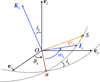 |
Fig. 3 Frame of reference ℛs: (O, Is, Js, Ks) and Keplerian elements describing the orbit of the perturber. |
3.2 Dynamical equations
The planet’s spin angular velocity is typically much greater than the variation rates of the precession and nutation angles introduced in Eq. (1) as α and β, respectively. Mathematically,  and
and  . As a result, the gyroscopic approximation can be applied (see e.g. Boué & Efroimsky 2019, Sect. 2.8), which involves disregarding the contributions of the terms related to
  and
and  in the calculation of the planet’s angular momentum, Lp. Under this approximation, Lp is simply expressed as
 (66)
(66)
where C designates the principal moment of inertia of the planet, and Ω ∈ ΩeZ its spin vector. The evolution rate of the planet’s angular momentum is the tidal torque established in Eqs. (58–60),
 (67)
(67)
Expanding  in terms of Ω, α and β, and using the basis unit vectors introduced in Sect. 2.1 and Fig. 1, we obtain
 (68)
(68)
which, owing to the orthogonality of the vectors, eZ, ez × eZ, and e′y × eZ, yields the variation rates of Ω, α, and β,
 (69)
(69)
Analogously with Lp, the angular momentum of the satellite’s orbit, Ls, is defined as
 (70)
(70)
and its variation rate is expressed as
 (71)
(71)
Thus, expanding  in terms of the Euler angles describing the inclination of the orbit, αs and βs (see Eq. (63)), we end up with
 (72)
(72)
and the variation rates of Ls, αs, and βs,
 (73)
(73)
We remark that all the equations established until now are general and do not depend on the choice made for the fixed frame of reference (ℛf ).
It is actually appropriate to define ℛf so that ez is aligned with the total angular momentum of the two-body system,
 (74)
(74)
with the vectors ex and ey defining the so-called invariable plane; namely, the plane perpendicular to the total angular momentum (e.g. Tremaine et al. 2009; Rubincam 2016; Boué et al. 2016; Boué & Efroimsky 2019). In this configuration, α − αs = π, which allows the evolution equations of the set of variables {Ω, Ls, β, βs} to be deduced from Eqs. (69) and (73),
![$\dot \Omega = {C^{ - 1}}\left[ {\sin \beta \left( {\cos \alpha {{\cal T}_x} + \sin \alpha {{\cal T}_y}} \right) + \cos \beta {{\cal T}_z}} \right]$](/articles/aa/full_html/2025/02/aa53019-24/aa53019-24-eq115.png) (75)
(75)
 (76)
(76)
![$\dot \beta = {(C\Omega )^{ - 1}}\left[ {\cos \beta \left( {\cos \alpha {{\cal T}_x} + \sin \alpha {{\cal T}_y}} \right) - \sin \beta {{\cal T}_z}} \right],$](/articles/aa/full_html/2025/02/aa53019-24/aa53019-24-eq117.png) (77)
(77)
![${\dot \beta _{\rm{s}}} = L_{\rm{s}}^{ - 1}\left[ { - \cos {\beta _{\rm{s}}}\left( {\cos {\alpha _{\rm{s}}}{{\cal T}_x} + \sin {\alpha _{\rm{s}}}{{\cal T}_y}} \right) + \sin {\beta _{\rm{s}}}{{\cal T}_z}} \right].$](/articles/aa/full_html/2025/02/aa53019-24/aa53019-24-eq118.png) (78)
(78)
The perturber’s semi-major axis and eccentricity can be obtained from energy conservation principles. The total energy of the system, Etot, is formulated as
 (79)
(79)
where Es designates the mechanical energy of the perturber’s motion; and its variation rate as  . Since the power transferred from the planet’s spin to the planet’s orbital motion is expressed as
 (80)
(80)
taking the time derivative of Eq. (79) yields the relationship
 (81)
(81)
The semi-major axis of the perturber is readily deduced from Es (e.g. MacDonald 1964),
 (82)
(82)
Analogously, the angular momentum of the perturber is given by (e.g. MacDonald 1964)
 (83)
(83)
which allows the eccentricity to be expressed as a function of the other quantities,
 (84)
(84)
We remark that the tangential component of Ltot is zero by construction, given that Ltot is aligned with ez in the adopted frame of reference. Consequently, the tangential components of Lp and Ls exactly compensate each other, which is formulated as
 (85)
(85)
The equatorial plane of the planet and the orbital plane of the perturber are thus inclined in two opposite directions, and the angle, βs, can be deduced from β, Ω, and Ls,
 (86)
(86)
Similarly, Ltot appears to be a first integral of the problem, as no external torque acts on the system. The constancy of Ltot over time  imposes an additional constraint on Ω, Ls, β, and βs, expressed by the equation
 (87)
(87)
This constraint can be used to verify the consistency of the system’s dynamical evolution over time, as the left-hand side must remain unchanged despite variations in Ω, Ls, β, and βs. The system’s evolution is then determined by integrating Eqs. (75–77) and Eq. (80) for {Ω, β, Ls, Es}. The quantities as, es, and βs are subsequently derived from the former using the relations provided in Eqs. (82), (84), and (86), respectively.
4 Application to the Earth–Moon system
4.1 Physical set-up of tidal solutions
In the previous sections, we derived the general expressions of tidal torque and power as functions of the forcing and deformation tidal potentials, incorporating the non-isotropic effects that are usually ignored. This formalism now enables us to investigate, as a next step, how deviations from the isotropic assumption may alter the estimates of these quantities and potentially lead to inaccurate predictions regarding the evolution of planetary systems.
For a didactical purpose, we applied the described methods to an idealised Earth-Moon system. The Earth was modelled as a two-layer, spherically symmetric body with a massive solid part and a thin, uniformly deep liquid water ocean, with a depth of H << Rp. The formalism used to compute the linear tidal response of such a planet has been extensively detailed in previous works (Auclair-Desrotour et al. 2018, 2019; Farhat et al. 2022b; Auclair-Desrotour et al. 2023). Therefore, we shall only briefly outline the key aspects of the approach followed here and direct readers to these studies for further details.
As is outlined in Auclair-Desrotour et al. (2023), the tidal response of the Earth’s solid part is modelled using Andrade rheology, with parameter values prescribed by Bolmont et al. (2020) for the actual Earth. Andrade rheology captures both viscoelastic and inelastic deformations of the solid regions. Although initially developed from lab experiments on metals (Andrade 1910), later studies demonstrated its applicability to silicate rocks and ices (see e.g. Efroimsky 2012b, and references therein). In this framework, the tidal response of the solid Earth is governed by the mantle’s effective shear modulus, µ, the Maxwell time, τM, which parametrises viscous friction, and two additional parameters linked to inelastic elongation: the Andrade time, τA, and a dimensionless parameter, α, which characterises the unrecoverable creep (e.g. Castelnau et al. 2008; Castillo-Rogez et al. 2011; Efroimsky 2012b). The latter parameter scales the frequency-dependent energy dissipation in the high-frequency regime.
The Andrade model is believed to accurately represent the tidal response of rocky bodies such as terrestrial planets and icy satellites, particularly in the high-frequency range where inelasticity dominates (e.g. Efroimsky & Lainey 2007). However, alternative models can also be applied (see e.g. Henning et al. 2009). The detailed computation of the solid Love numbers is presented in Auclair-Desrotour et al. (2023), Appendix H. This approach is based on Kelvin’s closed-form solution for an incompressible, homogeneous sphere (e.g. Munk & MacDonald 1960, Chapter 5). Here, we have employed this simplified model as a general method to describe the contribution of solid tides to energy dissipation in Earth-like scenarios, in which oceanic tides are predominant. Nevertheless, the calculation of the solid Love numbers can be refined later using more sophisticated methods based on elasto-gravitational theory (e.g. Takeuchi & Saito 1972; Tobie et al. 2005), along with realistic radial profiles of material properties (e.g. Sotin et al. 2007).
The oceanic tidal theory used here follows the approach detailed in Auclair-Desrotour et al. (2023). The ocean’s tidal response was obtained by solving the linear Laplace tidal equations (hereafter LTEs) over a spherical surface. Originally formulated by Laplace in his ‘Traité de Mécanique Céleste’ (Laplace 1798, Book IV), these equations were given a modern formulation in the foundational work by Longuet-Higgins (1968). We considered the LTEs in the shallow water approximation, in which tidal variables are depth-averaged (Vallis 2006). In this approach, the tidal solution reduces to barotropic tidal flows – those independent of vertical structure – which are dominant on Earth (Gerkema 2019). It represents planetary-scale surface gravity waves, restored by variations in self-attraction due to local ocean surface elevation (Vallis 2006). These waves are directly forced by the tide-raising potential, with their typical phase speed given by  (e.g. Cartwright 1977).
Consequently, vertical oceanic structure effects on tidal dynamics are neglected, meaning the contribution of internal gravity waves (i.e. waves restored by the Archimedean force; e.g. Gerkema et al. 2008) is formally excluded. However the impact of these waves is implicitly accounted for in the effective damping caused by dissipative processes. Using high-resolution TOPEX/Poseidon altimetric data, Egbert & Ray (2000) and Egbert & Ray (2001) demonstrated that energy dissipation on Earth primarily arises from bottom drag in shallow seas (~70%) and barotropic-to-baroclinic tidal conversion in deep oceans (25–35%). This conversion results from internal gravity waves generated by the interaction between tidal flows and ocean floor topography (Bell Jr 1975; Jayne & St. Laurent 2001; Garrett & Kunze 2007).
The LTEs consist of the horizontal momentum and continuity equations of fluid dynamics linearised for tidal perturbations, which are assumed to be small disturbances relative to the background fields (see e.g. Hay & Matsuyama 2019, for an exhaustive formulation of the LTEs including non-linear terms). These equations are expressed, respectively, as (e.g. Hendershott 1972; Matsuyama 2014; Matsuyama et al. 2018; Auclair-Desrotour et al. 2023)
 (88)
(88)
 (89)
(89)
where  is the planet’s surface gravity, σR is the Rayleigh drag frequency accounting for the efficiency of dissipative processes, and
 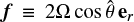 denotes the Coriolis parameter, with er being the outward-pointing radial unit vector. Here, V represents the horizontal velocity field, ζ the vertical displacement of the ocean’s surface relative to the ocean floor, and ζeq = UT/𝑔 the equilibrium displacement caused by the tidal gravitational potential in the zero-frequency limit.
For simplification, mean flows are ignored in Eq. (88), treating the ocean as a static fluid layer. This assumption is based on the separation of spatial scales and timescales between tidal and mean flows, with the latter characterised by smaller spatial structures and longer timescales, reducing the likelihood of significant coupling. However, this assumption does not always hold for thick fluid envelopes, where large-scale circulation patterns, such as differential rotation or latitudinal shear, can affect tidal flows by inducing Doppler-shift effects (e.g. Boyd 1978; Ortland 2005a,b; Baruteau & Rieutord 2013; Guenel et al. 2016). While permanent oceanic currents are generally thought to have minimal impact on tidal dynamics, they are influenced by tidal energy dissipation and internal waves, which interact with oceanic mesoscale eddies (see e.g. Arbic 2022, and references therein).
The Rayleigh drag frequency, σR, plays a crucial role as it governs the frequency-dependent rates of energy and momentum exchanges within the planet-perturber system. As σR decreases, both energy and momentum transfer rates become more sensitive to tidal frequency (e.g. Auclair-Desrotour et al. 2018). This behaviour is linked to the phenomenon of the dynamical tide, which refers to the component formed by forced tidal waves propagating through a fluid layer (Zahn 1975). In this context, the dynamical tide results from long-wavelength surface gravity waves, which can be resonantly excited by the tide-raising potential, leading to significant variations in the tidally dissipated energy (e.g. Webb 1980; Tyler 2014, 2021; Kamata et al. 2015; Auclair-Desrotour et al. 2018, 2019, 2023; Matsuyama et al. 2018; Hay & Matsuyama 2019; Farhat et al. 2022b; Rovira-Navarro et al. 2023). As σR diminishes, the strength of the dynamical tide increases, with the height of resonant peaks scaling as  in linear theory (see e.g. Auclair-Desrotour et al. 2019, Eq. (58)).
This relationship generally holds for fluid bodies. The frequency dependence of the tidal response driven by forced wave propagation in planetary fluid layers and stars becomes more pronounced as the damping coefficient for frictional forces (or other dissipative mechanisms) decreases. This can result in energy dissipation rates that span several orders of magnitudes in stars and giants planets (e.g. Savonije & Witte 2002; Ogilvie & Lin 2004, 2007; Ogilvie 2009, 2013; Auclair Desrotour et al. 2015; Mathis et al. 2016; Astoul & Barker 2023), or in the sub-surface oceans of icy moons (Tyler 2011, 2014; Chen et al. 2014; Matsuyama 2014; Matsuyama et al. 2018; Beuthe 2016). Rayleigh drag frequency is typically unconstrained and can vary widely. For instance, Matsuyama et al. (2018) report values as low as σR ~ 10−11 s−1 for icy moons in the Solar System, with σR ~ 10−9 s−1 for obliquity tides on Europa. In the present study, we adopt σR = 10−5 s−1, in line with estimates reckoned from high-precision measurements of Earth’s tidal energy dissipation and advanced tidal models (e.g. Webb 1980; Egbert & Ray 2001, 2003; Farhat et al. 2022b). Given the strong sensitivity of tidal dissipation to σR, this value represents a conservative estimate for examining the impact of anisotropy on tidal dissipation. Any smaller value would amplify the frequency dependence of the oceanic tidal response.
The operators, ΓD and ΓT, in Eq. (88) account for ocean loading, self-attraction, and the deformation of the planet’s solid regions, which slightly modify the oceanic tidal response (e.g. Hendershott 1972; Ray 1998; Egbert et al. 2004). These operators are expressed in the frequency domain as functions of the solid tidal and load Love numbers, as is detailed in Auclair-Desrotour et al. (2023). Also, it is important to note that the three-dimensional gradient operator, ∇, introduced in Eq. (7), is applied over the spherical surface in Eq. (88), along with the divergent operator, ∇· in Eq. (89). These operators are explicitly formulated in spherical coordinates in Appendix B. Equations (88) and (89) are solved for the velocity field, V, and ocean surface displacement, ζ, in the frequency domain for every component of the tide-raising gravitational potential expressed in the rotating frame of reference, as is provided by Eq. (27). This potential is computed using Eq. (65), with the degree-2 truncation (l ≤ 2) corresponding to the classical quadrupolar approximation (e.g. Mathis et al. 2013, Sect. 7.2.2.5).
Following the approach of Auclair-Desrotour et al. (2023), we numerically solved the LTEs by employing a spectral method that expands the tidal quantities in spherical harmonics series. Specifically, using the notations introduced in Sect. 2.2, the variations in ocean depth are expressed as
 (90)
(90)
The spatial functions  are further expanded as
 (91)
(91)
where  are the complex coefficients of the multipole expansion and N denotes the truncation degree of the series. As discussed in Appendix H from a convergence analysis, the truncation degree in Eq. (91) is set to N = 30. This value empirically appears to be sufficiently large to account for the complex mapping between the ocean’s forced modes and spherical harmonics.
Finally, from the solution, we derived the Fourier coefficients of the deformation tidal potential needed to evaluate the tidal torque and power, as is formulated in Eqs. (58–61). These coefficients, introduced in Eq. (32), are expressed in terms of the components of the tide-raising potential and the variation in ocean depth, as is shown in (e.g. Auclair-Desrotour et al. 2023, Eq. (72))4,
 (92)
(92)
where  denotes the planet’s mean density, ρw ≈ 1035 kg m−3 represents the average density of seawater (e.g. Ray et al. 2001), and
  and
and  are the complex solid tidal and load Love numbers that describe the visco-elastic deformation of solid regions at the frequency
  . The first term on the righthand side of Eq. (92) accounts for the solid elongation caused by the forcing tidal potential. The second term captures the contribution of oceanic tides to self-attraction variations, consisting of two components: the gravitational potential created by surface elevation changes and the deformation of solid regions due to ocean loading.
4.2 Sensitivity of tidal dissipation to planet’s spin rotation and obliquity
In our calculations, we assume that the perturber causing the tidal forcing is a Lunar-mass satellite in a circular orbit around the planet (es = 0), with the same semi-major axis as the current Earth-Moon system, and a fixed orbital period, Ps. The planet’s rotation period, Prot, is varied from 0.1 to 100 days, and its obliquity, β, from 0° to 90°. We investigated two configurations. In the first configuration (‘DRY’), the ocean was neglected, and only the solid tide was considered. In the second configuration (‘GLOBAL OCEAN’), the full tidal response, including the ocean, was evaluated. For each configuration, the calculations were performed in two scenarios: (i) using the full formalism introduced in Sect. 2, where the planet’s tidal response is computed comprehensively and self-consistently (‘FULL’), and (ii) under the classical isotropic approximation, where all tidal components are derived from the equatorial degree-2 Love number defined in the circular-coplanar configuration for the semidiurnal tide (’APPROX’). We computed the tidal solutions using the numerical tools of the TRIP software (Gastineau & Laskar 2011)5.
In the APPROX case, the equatorial degree-2 Love number was calculated for every tidal frequency of the forcing potential in the planet’s rotating frame. Each tidal frequency, σ, was treated as a semidiurnal tidal frequency, σ = 2 (Ω − ns), where the fictitious orbital frequency is defined as ns = Ω − σ/2. The corresponding tidal response was then evaluated using the spatial distribution for the semidiurnal quadrupolar tidal potential, represented by the spherical harmonic of degree 2 and order 2 (denoted by  ). From the resulting solution, the degree-2 Love number was derived and used to compute the deformation potential for the relevant tidal component. This potential is simply the product of the degree-2 Love number and the tide-raising potential, following the theory of bodily tides. It is important to note that the Love number depends solely on σ in the dry configuration due to the spherical isotropy of the solid part. However, in the global ocean configuration, it also depends on the planet’s spin period because of the influence of Coriolis forces, as was described earlier.
Figures 4, 5, and 6 present the results for tidally dissipated power (𝒫diss), the variation rate of the planet’s spin angular velocity (Ω), and the variation rate of the planet’s obliquity  , respectively. Additionally, the relative difference between the two cases (FULL and APPROX), denoted by η, is shown for each configuration and for the three quantities (bottom panels). This difference is normalised by the values obtained in the full calculation. For a given tidal quantity, f, the relative difference is defined mathematically as
 (93)
(93)
where ffull and fapprox represent the values obtained in the FULL an APPROX cases, respectively.
We first examined the solid-body configuration (Figs. 4–6, left panels). In this scenario, the three quantities − 𝒫diss,  – vary smoothly with changes in the planet’s rotation period and obliquity. In the coplanar case (β = 0°), both the tidally dissipated power and the variation rate of spin velocity approach zero as the planet crosses the 1:1 spin-orbit resonance (Prot = Ps). As obliquity increases, obliquity tides become more dominant, shifting the equilibrium states. Due to the spherical isotropy of the solid part, the results from the FULL and APPROX calculations are identical, leading to a relative difference of zero between the two approaches.
At higher obliquities, obliquity tides can induce an additional equilibrium state corresponding to the 2:1 spin-obit resonance (Prot = Ps/2), which is particularly visible in Fig. 5. In this configuration, the frequency of the quadrupolar obliquity component of the tidal potential (σ = Ω − 2ns, and m = 1) becomes zero. Both the 1:1 and 2:1 resonances are indicated by dashed magenta lines in Fig. 4 (top right panel). It is worth noting that the solid part’s ability to dissipate energy via viscous friction is maximised at very low tidal frequencies, given that typical Maxwell timescales for rocky planets reach several centuries (Peltier 1974; Karato & Spetzler 1990; Bolmont et al. 2020). Consequently, any change in the sign of a tidal frequency results in a sharp variation in the associated tidal component.
When the global ocean is included in the tidal response, long- wavelength surface gravity modes can be resonantly excited by tidal forces. This greatly increases the sensitivity of both dissipated power and tidal torque to the planet’s rotation period. The resonant peaks of these modes occur at specific frequencies, given by (e.g. Longuet-Higgins 1968; Lee & Saio 1997; Auclair-Desrotour et al. 2023)
 (94)
(94)
In this equation, ν ≡ 2Ω/σ is the spin parameter, and  represents the eigenvalues associated with the Hough functions that describe the horizontal structure of the forced oceanic eigenmodes. Hough functions are essentially spherical harmonics modified by the planet’s rotation (e.g. Longuet-Higgins 1968; Lindzen & Chapman 1969; Lee & Saio 1997; Wang et al. 2016). These functions arise from the LTEs and were first introduced by Hough in his pioneering work (Hough 1898).
The most prominent peaks observed in Figs. 4–6 are caused by the semidiurnal tide (i.e. σ = 2 (Ω - ns) with m = 2). These peaks appear as long as the tidal frequency exceeds the eigenfrequency corresponding to the longest-wavelength gravity mode (n = 2). In the regime in which oceanic modes become resonant, ns « Ω, so the semidiurnal tidal frequency simplifies to σ ≈ 2Ω, implying that ν ≈ 1. Consequently, the spin rotation periods at which resonances occur can be expressed as
 (95)
(95)
with n = 2,4,6,…, +∞. The eigenvalues and corresponding rotation periods for the main resonances are listed in Table 2, and these resonances are indicated by dashed green lines in Fig. 4 (top right panel).
In the resonant regime, the oceanic dynamical tide greatly enhances the energy dissipated through tidal forces, as well as the rates of change of spin angular velocity and obliquity. The amplification factor associated with a resonance is directly related to the efficiency of tidal flow drag against the ocean floor. Typically, the maximum tidal torque during a resonance crossing scales as œ 1/σR in the adopted linear model (see e.g. Auclair-Desrotour et al. 2019, Eqs. (55) and (58)). Using the drag frequency inferred from Earth’s present tidal energy dissipation, the torque can be resonantly amplified by approximately an order of magnitude (Webb 1980; Auclair-Desrotour et al. 2023). The strength of these resonances also depend on the overlap coefficients between Hough functions and spherical harmonics, which vary with the planet’s obliquity and the orbital inclination of the perturbing body. Furthermore, the geometry of the ocean basin influences the coupling between the excited oceanic modes and the tidal forcing potential. Continental coastlines introduce more resonant peaks compared to the global ocean scenario studied here, as is discussed in Auclair-Desrotour et al. (2023). The interactions between tidal flows and coastlines also enable the resonant excitation of modes with lower eigenfrequencies.
Next, we considered the divergences between the FULL and APPROX cases when oceanic tides are included. These discrepancies are evident in the plots showing the evolution of tidally dissipated power and the rate of change of spin angular velocity (Figs. 4 and 5, top and middle right panels). In the FULL case, the peaks associated with oceanic equatorial gravity modes tend to diminish as the obliquity increases, consistent with the decreasing coupling between these modes and the tidal forcing. Gravity modes are progressively replaced by non-resonant polar waves.
Conversely, in the APPROX case, new peaks emerge as the obliquity increases. Notably, the two solutions diverge significantly for a planet with a 10-hour rotation period (log (Prot) = −0.380 where Prot is in days). These new peaks are artefacts arising from the assumption that the planet’s tidal response is independent of its orientation relative to the perturber’s orbit. This assumption artificially reproduces resonances linked to equatorial gravity modes in scenarios in which these modes are, in reality, subdominant. As a result, the APPROX model can overestimate the tidal torque on the planet by several orders of magnitude, leading to regions of the parameter space with substantial errors (η ≥ 1), as is shown by Figs. 4 and 5 (bottom panels). It should be noted that in these regions, η may exceed 1 by a considerable margin, as it is directly related to the resonant amplification factor, which is a function of σR. The error introduced by this approximation, particularly regarding the degree-2 Love number, is even more pronounced for the rate of change of obliquity. This is evident from Fig. 6 (bottom right panel), where the inaccurate predictions of the APPROX model extend over a broad area of the parameter space, including configurations with near-zero obliquity.
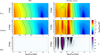 |
Fig. 4 Tidally dissipated power (𝒫diss) as a function of the planet’s spin rotation period (horizontal axis) and obliquity (vertical axis) for Earth-sized dry (left panels) and global-ocean (right panels) planets. Top: full calculation of the planet’s tidal response (FULL). Middle: calculation using, for all tidal forcing terms, the degree-2 Love number computed in the equatorial plane assuming the coplanar-circular configuration (APPROX). Bottom: relative difference between the FULL and APPROX cases, defined by Eq. (93). The tidally dissipated power was computed from the tidal power and torque using Eq. (81). The dashed green lines indicate the resonances associated with the oceanic surface gravity modes (see Eq. (95) and Table 2), and the dashed magenta lines the 1:1 and 2:1 spin-orbit resonances. The black dot at (Prot, β) = (1 day, 0°) designates the actual Earth-Moon system in the coplanar-circular approximation. |
 |
Fig. 5 Variation rate of the planet’s spin angular velocity (Ω) as a function of the planet’s spin rotation period (horizontal axis) and obliquity (vertical axis) for Earth-sized dry (left panels) and global-ocean (right panels) planets. Top: full calculation of the planet’s tidal response (FULL). Middle: calculation using, for all tidal forcing terms, the degree-2 Love number computed in the equatorial plane assuming the coplanar-circular configuration (APPROX). Bottom: relative difference between the FULL and APPROX cases, defined by Eq. (93). The variation rate of the planet’s spin angular velocity was computed from the three-dimensional tidal torque using Eq. (75). The black dot at (Prot,β) = (1 day, 0°) designates the actual Earth-Moon system in the coplanar-circular approximation. |
Values of parameters used in our case study.
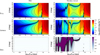 |
Fig. 6 Variation rate of the planet’s obliquity |

Features of the global ocean modes that are resonantly excited by the semidiurnal tidal forces.
4.3 Spatial distributions of tidal self-attraction variations
To visualise how the solution is altered in the APPROX case, we considered the gravitational potential induced by the ocean’s elevation in the rigid-body limit, where solid regions are non- deformable. This potential is generally expressed by Eq. (20).
However, terms where q ≠ p can be discarded, since the frequencies associated with these terms (σk,q,p) differ from those of the tide-raising potential (σk), as is given in Eq. (19), preventing their coupling with the forcing components on average. Therefore, only components of UD with q = p were considered. Furthermore, the Galilean frame of reference is not the most suitable for plotting UD, as tidal deformations follow the perturber, which moves in this frame. Instead, we plot the deformation tidal potential in a frame that rotates with the perturber, with the planet’s centre of gravity as its origin. This rotating frame uses spherical coordinates  , where
  , and
, and  corresponds to the direction of the angular momentum vector of the satellite’s orbit, Ls, as is introduced in Eq. (70). In this system,
  marks the sub-satellite point. It is important to note that the coordinate notations used here to describe the frame following the perturber are the same as those for the planetrotating frame in Sect. 2.2, so the two systems should not be confused.
The steps for transitioning from (r, θ, φ) to  are detailed in Appendix I. This yields the expression
 (96)
(96)
where the spatial functions,  , are given by
 (97)
(97)
In this equation, the complex coefficients,  , are expressed using the weighting coefficients introduced in Eq. (24) as
 (98)
(98)
We remark that the dominant component in Eq. (96) is static (q = 0), while the other components travel either eastwards (q < 0) or westwards (q > 0) relative to the sub-satellite point. At the planet’s surface  , the amplitude of UD is upper-bounded (superscript UB) by
 (99)
(99)
We calculated | UD|UB using both the FULL and APPROX models, considering obliquities ranging between 0° and 90° and two spin rotation periods: Prot = 33 h and Prot = 10 h. The first period corresponds to the rotation rate at which the primary oceanic mode is resonantly excited by the semidiurnal tide (see Table 2, n = 2). The second falls within the parameter space where the FULL and APPROX models significantly diverge. The remaining physical parameters were set to the values used for generating the solutions in Figs. 4–6, as is detailed in Table 1. The upper bound of the tidal potential, as is defined in Eq. (99), is plotted against the coordinates  in Fig. 7 for Prot = 33 h, and in Fig. 8 for Prot = 10 h. We note that the tidal potential is truncated at l = 2 (quadrupolar approximation), as the contribution from higher-degree terms to tidal dissipation is negligible when Rp ≪ as. Consequently, the smaller horizontal structures in the tidal potential are not visible in the colour maps, although they are accounted for in the tidal solutions.
For Prot = 33 h (Fig. 7), the dominant pattern arises from the resonantly excited equatorial gravity mode in both the FULL and APPROX cases, resulting in the two solutions appearing largely similar. The slight differences observed are due to errors in calculating the oceanic obliquity tides within the APPROX model, but these discrepancies remain minor compared to the semidiurnal tidal component. This component is represented in the colour maps generated for the coplanar-circular configuration, where the two solutions are identical (see Fig. 7, bottom panels). At Prot = 10 h (Fig. 8), the semidiurnal oceanic tide is weak, as no equatorial gravity mode is excited by the associated forcing potential. As a result, the tidal response is more sensitive to obliquity tides compared to Prot = 33 h. Moreover, the APPROX model artificially reproduces the resonance of an equatorial gravity mode for an obliquity tidal component, leading to an amplification of this component by an order of magnitude. Consequently, the FULL and APPROX solutions show substantial divergence for non-zero obliquities, consistent with the large errors observed in estimates of tidally dissipated power, and the variation rates of spin angular velocity and obliquity (Figs. 4–6, bottom right panels).
As is discussed in Appendix J, the spatial distribution of the deformation tidal potential, shown in Figs. 7 and 8, is strongly influenced by the elasticity of solid regions. In the rigid limit considered here, variations in self-attraction are solely generated by oceanic tides, which display complex horizontal structures due to the excitation of modes of various degrees. This helps to clarify the causes of the discrepancies observed in the tidally dissipated power and the variation rates of the planet’s spin angular velocity and obliquity between the FULL and APPROX cases. When solid elasticity is taken into account, as is seen in Figs. 4–6, the tidal bulge is primarily shaped by the degree-2 visco-elastic deformation of solid regions, driven by the density contrast between rocks and liquid water. Consequently, the deformation potential exhibits similar patterns in both the FULL and APPROX models. Although this may seem counterintuitive, the sensitivity of the planet’s tidal distortion to solid elasticity has a minimal effect on the tidally dissipated power and torque. This is because the angular lag induced by viscous friction in solid regions is much smaller than that of the oceanic tide in the configurations studied. This point is further explored in Appendix J, in which we use a toy model to illustrate the underlying mechanisms.
The primary limitations of our approach originate in the simplified geometry used to compute tidal solutions. Our model assumes a global surface layer with uniform depth, which overlooks the complex coupling between shallow seas and deep oceans that help damping resonances on Earth (e.g. Brian K. Arbic & Garrett 2009; Arbic & Garrett 2010). Furthermore, the intricate interactions between tidal flows and coastlines, which significantly impact tidal dissipation, are not considered. Additionally, non-linear processes generally inhibit the dynamical tide. For example, bottom friction between tidal flows and the ocean floor, which dominates on Earth, is a quadratic function of the velocity field (Egbert & Ray 2001, 2003). This tends to mitigate the predictions of linear tidal theory by smoothing out resonant peaks.
Nevertheless, even in the presence of non-linearities, which may significantly attenuate tidal energy transfer rates, dissipation remains strongly dependent on tidal frequency in stars and the fluid envelopes of giant planets due to the dynamical tide (e.g. Astoul & Barker 2022, 2023). As a result, the resonant amplification mechanism highlighted is equally applicable to fluid bodies beyond ocean planets. Finally, it is important to note that any symmetry-breaking effect, in addition to Coriolis forces, would increase scattering and make the tidal response more sensitive to the orientation of both the central body and the perturber’s orbit, causing the system to deviate further from the isotropic assumption.
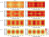 |
Fig. 7 Gravitational potential induced by the tidal response of an ocean planet with rigid solid regions in the system of coordinates rotating with the perturber for Prot = 33 h and obliquity values ranging between 0° and 90°. Left: maximum amplitude of the tidal potential obtained from the full calculation (FULL). Right: maximum amplitude of the tidal potential obtained with the standard approximation based on the equatorial degree-2 Love number (APPROX). Amplitudes are plotted as functions of longitude, |


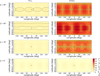 |
Fig. 8 Gravitational potential induced by the tidal response of an ocean planet with rigid solid regions in the system of coordinates rotating with the perturber for Prot = 10 h and obliquity values ranging between 0° and 90°. Left: maximum amplitude of the tidal potential obtained from the full calculation (FULL). Right: maximum amplitude of the tidal potential obtained with the standard approximation based on the equatorial degree-2 Love number (APPROX). Amplitudes are plotted as functions of longitude, |


5 Conclusions
In this study, we have explored how anisotropy influences the tidal response of fluid bodies, focussing specifically on Earthsized rocky planets with global oceans. Building on previous research that sought to deepen our understanding of oceanic tides and their role in the long-term evolution of the Earth-Moon system and exoplanets with liquid surface layers (Auclair-Desrotour et al. 2018, 2019, 2023; Farhat et al. 2022b), we examined the implications of a commonly used approximation. This approximation involves using the equatorial degree-2 Love number of the semidiurnal tide to quantify energy and angular momentum exchange rates across all components of the tidal response. By assuming spherical isotropy, it presumes that the Love number’s dependence on tidal frequency is uniform, regardless of the body’s orientation relative to the perturber’s orbit. Given that the isotropic assumption does not hold for stars and planetary fluid layers due to Coriolis forces, our primary goal is to assess the impact of this approximation on planetary evolution models, where it is frequently employed.
Our calculations are grounded in linear theory and the conventional framework of two-body tidal interactions. Using angular momentum theory, we first derived expressions for the time-averaged rate of energy exchange and the three-dimensional tidal torque as functions of the complex coefficients that describe the spherical harmonic expansions of tidal forcing and deformation potentials (Eqs. (58–61)). These expressions are general and apply even to non-isotropic bodies, enabling the computation of the long-term tidal evolution of planet-satellite or star-planet systems in three dimensions. For completeness, we also provided the variation rates of the planet’s spin angular velocity and the orbital elements of the perturber within this formalism.
We then applied the theory to an idealised Earth-Moon system. In this set-up, Earth is treated as a rocky planet with a thin, uniform-depth ocean at its surface, while the Moon is modelled as a point-mass satellite, following Auclair-Desrotour et al. (2023). We calculated the evolution of tidally dissipated energy as a function of the planet’s spin period and obliquity, both with and without the aforementioned Love number approximation. By comparing the two approaches, we quantified the error induced by this approximation in tidal models. Our results indicate that the error can be significant for ocean planets, as resonances associated with tidally forced oceanic modes greatly amplify it. In Earth-like configurations, the approximated model can overestimate tidally dissipated energy and angular momentum exchange rates by an order of magnitude, especially when tidal frequencies exceed the eigenfrequency of the ocean mode with the largest wavelength.
Interestingly, the Love number approximation does not uniformly affect the variation rates that describe the planetsatellite’s dynamical evolution. For instance, the variation rate of obliquity is significantly altered even in quasi-coplanar configurations (in which the perturber’s orbit lies nearly in the planet’s equatorial plane), whereas the tidally dissipated energy and the planet’s spin rate remain largely unaffected for obliquities under approximately ~10°. However, the extensive region of parameter space where the approximation fails for rotation periods shorter than one day suggests that it is unsuitable for studying the past evolution of the Earth-Moon system. In such cases, the tidal response should be computed self-consistently for each tidal component to properly account for scattering effects of Coriolis forces and continental coastlines, which enable the resonant excitation of lower-frequency modes.
These conclusions can be extended to stars and the fluid envelopes of gaseous giants, where the dynamical tide is typically the dominant component of the tidal response. However, the approximation remains valid in the non-wavelike regime, in which fluid waves cannot be resonantly excited by tidal forces. Additionally, the model used in this study, which is based on simplified geometry and linear tidal theory, has its limitations. Specifically, the propagation of forced tidal modes may be hindered by non-linear processes such as bottom friction, as well as by the complexity of land-ocean distributions and bathymetry. Therefore, while our findings provide valuable qualitative insights, they should be refined in future studies depending on the specific problem at hand.
Acknowledgements
The authors are thankful to the referee, Robert Tyler, for his thoughtful comments, which helped to improve the manuscript. This research has made use of NASA’s Astrophysics Data System.
Appendix A Nomenclature
The notations introduced in the main text are listed below in order of appearance.
| LOD | Length of day | p. 1 |
 |
Potential Love number | p. 2 |
| l | Degree of the spherical harmonics | p. 2 |
| m | Order of the spherical harmonics | p. 2 |
| k2 | Degree-2 potential Love number under the isotropic assumption | p. 2 |
| Mp | Planet mass | p. 2 |
| Rp | Planet radius | p. 2 |
| Ms | Satellite’s mass | p. 2 |
| UT | Tide-raising gravitational potential | p. 2 |
| UD | Perturbed gravitational potential | p. 2 |
| ℛf | Galilean frame of reference | p. 3 |
| O | Planet’s centre of mass | p. 3 |
| ex, ey, ez | Cartesian unit vector associated with ℛf | p. 3 |
| r | Radial coordinate in ℛf | p. 3 |
| θ | Colatitude in ℛf | p. 3 |
| φ | Longitude in ℛf | p. 3 |
| r | Position vector of the current point | p. 3 |
| rs | Satellite’s position vector | p. 3 |
| er | Unit radial vector | p. 3 |
| ℛ | Frame of reference rotating with the planet | p. 3 |
| eX, eY, eZ | Cartesian unit vectors associated with ℛ | p. 3 |
 |
Radial coordinate in ℛ | p. 3 |
 |
Colatitude in ℛ | p. 3 |
 |
Longitude in ℛ | p. 3 |
| R | 3-2-3 Eulerian rotation matrix | p. 3 |
| Rn | Rotation matrix around the n-th axis | p. 3 |
| α | Planet’s precession angle | p. 3 |
| β | Planet’s nutation angle | p. 3 |
| γ | Planet’s intrinsic rotation angle | p. 3 |
| t | Time | p. 3 |
| Ω | Planet’s spin angular velocity | p. 3 |
| F | Gravitational force per unit mass | p. 3 |
| 𝒱 | Domain occupied by the planet | p. 3 |
| 𝒯 | 3D torque vector | p. 3 |
| dp. V | Infinitesimal volume element | p. 3 |
| ρ | Density | p. 3 |
| × | Cross product | p. 3 |
| ∇ | Gradient operator | p. 3 |
| G | Universal gravitational constant | p. 3 |
| ⟨f⟩ | Average of the function f over time | p. 3 |
| f | Any function of time | p. 3 |
| ℒ | Angular momentum operator | p. 3 |
| δρ | Tidal density variation | p. 3 |
| ∇2 | Laplacian operator | p. 3 |
| 𝒱* | Any simply connected domain including the planet and excluding the perturber | p. 3 |
| dS | Outward-pointing infinitesimal surface element vector | p. 4 |
| ∂𝒱* | Boundary of 𝒱* | p. 4 |
| 𝒯x | Time-averaged torque exerted about the x axis | p. 4 |
| 𝒯y | Time-averaged torque exerted about the y axis | p. 4 |
| 𝒯z | Time-averaged torque exerted about the z axis | p. 4 |
| 𝒫T | Time-averaged tidal power | p. 4 |
| 𝒫diss | Time-averaged tidally dissipated power | p. 4 |
| ℜ | Real part of a complex number | p. 4 |
| ℑ | Imaginary part of a complex number | p. 4 |
| i | Imaginary unit | p. 4 |
| k, q, p | Integers | p. 4 |
| σk | k-th forcing tidal frequency in ℛf | p. 4 |
| σk,q,p | Frequency of the tidal response defined by the triplet (k, q, p) in ℛf | p. 4 |
 |
Complex spatial distribution of the k-th component of the tide-raising potential | p. 4 |
 |
Complex spatial distribution of the (k, q, p)- component of the perturbed potential | p. 4 |
 |
Complex weighting coefficients of the spherical harmonic expansion of the k-th component of the tide-raising potential | p. 5 |
 |
Complex weighting coefficients of the spherical harmonic expansion of the (k, q, p)- component of the perturbed potential | p. 5 |
 |
Wigner D-functions | p. 5 |
 |
Conjugate of the complex number Z | p. 5 |
 |
Complex spherical harmonic coefficient of the component of the tide-raising potential associated with the frequency  in ℛ in ℛ |
p. 5 |
 |
Spatial distribution function of the component of the perturbed potential associated with the triplet (l, q, k) | p. 5 |
 |
Transfer function relating the degree-s, order- p harmonic of the k-th component of the perturbed potential to the degree-l, order- q harmonic of the same component of the tide-raising potential | p. 5 |
| δq,p | Kronecker delta function, such that δq,p = 1 if q = p and δq,p = 0 otherwise | p. 5 |
 |
Spatial distribution function of the component of the perturbed tidal potential associated with the frequency  in ℛ in ℛ |
p. 5 |
 |
Complex spherical harmonic coefficients of the component of the perturbed potential associated with the frequency  in ℛ in ℛ |
p. 5 |
| e+, e0, e- | Set of complex unit vectors | p. 6 |
| a+, a0, a- | Coordinates of any vector a in (e+, e0, e-) | p. 6 |
 |
Coefficients of the angular momentum operator in spherical harmonics | p. 6 |
| ℒx | x component of the angular momentum operator | p. 6 |
| ℒy | y component of the angular momentum operator | p. 6 |
| ℒz | z component of the angular momentum operator | p. 6 |
| 𝒰 | Component of ŨD that does not generate any torque in average | p. 6 |
| A, B | Two real functions of spatial coordinates and time | p. 6 |
 |
Two complex-valued time-oscillating functions | p. 6 |
| σ1, σ2 | Frequencies associated with à and  , respectively , respectively |
p. 6 |
 |
Complex spatial components of à and  , respectively , respectively |
p. 6 |
| K | Constant coefficient | p. 7 |
| as | Satellite’s semi-major axis | p. 7 |
| es | Satellite’s eccentricity | p. 7 |
| is | Satellite’s orbital inclination | p. 7 |
| υs | Satellite’s true anomaly | p. 7 |
| ϑs | Longitude of the ascending node | p. 7 |
| ωs | Argument of the pericentre | p. 7 |
| ℛs | Reference frame associated with the satellite’s orbit | p. 7 |
| Is | Unit vector pointing towards the pericentre of the satellite’s orbit | p. 7 |
| Ks | Unit vector aligned with the orbital angular momentum | p. 7 |
| Js | Third unit vector defined as Js = Ks × Is | p. 7 |
| αs, βs, γs | Euler angles describing the rotation ℛf: (O, ex, ey, ez) →:(O, Is, Js, Ks) | p. 7 |
| ℳs | Satellite’s mean anomaly | p. 7 |
 |
Hansen coefficients | p. 7 |
| ℳs;0 | Constant phase angle | p. 7 |
| Lp | Planet’s angular momentum vector | p. 7 |
| C | Planet’s principal moment of inertia | p. 7 |
| Ω | Planet’s spin vector | p. 7 |
| Ls | Satellite’s angular momentum vector | p. 8 |
| Ltot | Total angular momentum vector of the planet-satellite system | p. 8 |
| Etot | Total energy of the planet-satellite system | p. 8 |
| Es | Mechanical energy of the perturber’s motion | p. 8 |
| H | Ocean’s depth | p. 9 |
| µ | Mantle’s effective shear modulus | p. 9 |
| τM | Maxwell time | p. 9 |
| τA | Andrade time | p. 9 |
| α | Dimensionless parameter characterising the unrecoverable creep | p. 9 |
| LTEs | Laplace tidal equations | p. 9 |
| g | Planet’s surface gravity | p. 9 |
| σR | Rayleigh drag frequency | p. 9 |
| f | Coriolis parameter | p. 9 |
| V | Horizontal velocity field | p. 9 |
| ζ | Vertical displacement of the ocean’s surface relative to the ocean’s floor | p. 9 |
| ζeq | Equilibrium surface elevation in the zerofrequency limit | p. 9 |
| ΓD, ΓT | Operators accounting for ocean loading, selfattraction, and the deformation of the planet’s solid regions | p. 10 |
 |
Complex coefficients of the multipole expansion of ocean’s surface elevation in ℛ | p. 10 |
| N | Truncation degree of the spherical harmonic series in numerical solutions | p. 10 |
 |
Planet’s mean density | p. 10 |
| ρw | Average seawater density | p. 10 |
 |
Complex solid tidal Love numbers | p. 10 |
 |
Complex solid load Love numbers | p. 10 |
| Ps | Satellite’s orbital period | p. 10 |
| Prot | Planet’s rotation period | p. 10 |
| η | Relative difference between the FULL and APPROX cases for a quantity | p. 11 |
| v | Spin parameter | p. 12 |
 |
Eigenvalues associated with Hough functions | p. 12 |
| Pn | Rotation periods at which oceanic resonances occur | p. 12 |
| |UD|UB | Upper bound of the perturbed potential at planet’s surface | p. 14 |
Appendix B Vectorial operators in spherical coordinates
Throughout this study, we use the standard spherical coordinate system (r, θ, φ), where r denotes the radial coordinate, θ is the colatitude (the angle measured from the z-axis), and φ represents the longitude. In this coordinate system, the gradient of any scalar quantity f is expressed as (e.g. Arfken & Weber 2005, Sect. 2.5)
 (B.1)
(B.1)
where (er, eθ, eφ form the orthogonal basis of unit vectors corresponding to the spherical coordinates (r, θ, φ). The Laplacian of f is given by
 (B.2)
(B.2)
Similarly, the divergence of a vector field V = Vrer + Vθeθ + Vφeφ is expressed as
 (B.3)
(B.3)
When applying the gradient and divergence operators over a 2D spherical surface, as in Eqs. (88) and (89), the radial terms ∂r and ∂rr vanish. As a result, the gradient of f and the divergence of V = (Vθ, Vφ) simplify as follows:
 (B.4)
(B.4)
 (B.5)
(B.5)
Appendix C Time-averaged power
We demonstrate here how the time-averaged power, as defined by Eqs. (6) and (52), can be related to the complex Fourier coefficients of the relevant quantities, specifically using the formula given in Eq. (57). We consider two fields, A and B, which vary as functions of time and spatial coordinates and are expressed as the real parts of the complex fields à and  ,
,
 (C.1)
(C.1)
We assume that both à and  can be written as sinusoidal timeoscillations multiplied by complex spatial functions,
 (C.2)
(C.2)
From Eq. (6), the time-average of the product AB is defined as
 (C.3)
(C.3)
where P is the time interval over which the average is calculated. Expanding the real parts of à and  , we write
 (C.4)
(C.4)
 (C.5)
(C.5)
Now, expanding the product AB yields
 (C.6)
(C.6)

If σ1 ≠, σ2 and σ2 ≠, −σ1, we obtain
 (C.7)
(C.7)
indicating that there is no coupling between A and B. However, if σ1 = σ2 = σ, then
 (C.8)
(C.8)
We recognise this as the real part of the product  , expanded as
 (C.9)
(C.9)

which, when integrated over the spatial coordinates, gives Eq. (57).
Appendix D Legendre polynomials and spherical harmonics
The spherical harmonics  in Eqs. (23) and (24) are defined as (Varshalovich et al. 1988, Sect. 5.2, Eq. (1))
 (D.1)
(D.1)
where  denotes the associated Legendre functions (ALFs), defined for −1 ≤ x ≤ 1, with l and m as integers such that | m | ≤ l, as follows:
 (D.2)
(D.2)
In this equation, Pl represents the degree-l Legendre polynomial (Abramowitz & Stegun 1972, Eq. (8.6.18)), defined as
 (D.3)
(D.3)
The normalisation of the spherical harmonics  is given by the integral
 (D.4)
(D.4)
As specific value of the spherical harmonics,  , as used in Eq. (65) is expressed as
 (D.5)
(D.5)
where the double factorial of a positive integer n, denoted by n!!, is defined as
 (D.6)
(D.6)
with  representing the ceiling of n/2.
Appendix E Wigner D-functions
The Wigner D-functions introduced in Eqs. (25) and (26) represent the matrix elements of the rotation operator applied to spherical harmonics (Varshalovich et al. 1988, Sect. 4.1). They are structured as follows:
![${\bf{D}} \equiv \left[ {\matrix{ {{\bf{D}}_{0,0}^0} & 0 & \cdots & \cdots & \cdots & 0 \cr 0 & {{\bf{D}}_{q,m}^1} & \ddots & {} & {} & \vdots \cr \vdots & \ddots & \ddots & \ddots & {} & \vdots \cr \vdots & {} & \ddots & {{\bf{D}}_{q,m}^l} & \ddots & \vdots \cr \vdots & {} & {} & \ddots & \ddots & 0 \cr 0 & \cdots & \cdots & \cdots & 0 & {{\bf{D}}_{q,m}^N} \cr } } \right],$](/articles/aa/full_html/2025/02/aa53019-24/aa53019-24-eq232.png) (E.1)
(E.1)
where N indicates the chosen truncation degree, and  is the matrix
![${\bf{D}}_{q,m}^l \equiv \left[ {\matrix{ {D_{ - l, - l}^l} & \ldots & {D_{ - l,m}^l} & \ldots & {D_{ - l,l}^l} \cr \vdots & {} & \vdots & {} & \vdots \cr {D_{q, - l}^l} & \ldots & {D_{q,m}^l} & \ldots & {D_{q,l}^l} \cr \vdots & {} & \vdots & {} & \vdots \cr {D_{l, - l}^l} & \ldots & {D_{l,m}^l} & \ldots & {D_{l,l}^l} \cr } } \right].$](/articles/aa/full_html/2025/02/aa53019-24/aa53019-24-eq234.png) (E.2)
(E.2)
The Wigner D-functions,  , are defined as (Varshalovich et al. 1988, Sect. 4.3, Eq. (1))
 (E.3)
(E.3)
where  is a real function given by (Varshalovich et al. 1988, Sect. 4.3.1, Eq. (2))
 (E.4)
(E.4)
The summation index k runs over all integer values for which the factorial arguments are non-negative, namely max (0, −q − m) ≤ k ≤ min(l − q, l − m).
In practice, Wigner D-functions are computed recursively using the method described by Gimbutas & Greengard (2009), starting with
![${\bf{D}}_{0,0}^0 = 1,\quad {\bf{D}}_{q,m}^1 = \left[ {\matrix{ {{{\bar a}^2}} & { - \sqrt 2 \bar ab} & {{b^2}} \cr { - \sqrt 2 \bar a\bar b} & {a\bar a - b\bar b} & { - \sqrt 2 ab} \cr {{{\bar b}^2}} & { - \sqrt 2 a\bar b} & {{a^2}} \cr } } \right],$](/articles/aa/full_html/2025/02/aa53019-24/aa53019-24-eq239.png) (E.5)
(E.5)
where the Cayley-Klein parameters, a and b, are defined in terms of the 3-2-3 Euler angles from Eq. (1) as
 (E.6)
(E.6)
For matrices of degrees l ≥ 2, we use the recursion relation given by (e.g. Boué 2017, Sect. 2.5)6
 (E.7)
(E.7)
with the coefficients  and
and  defined as
 (E.8)
(E.8)
Terms  where |m + v| > l − 1, with ν ∊ {−1,0,1), are discarded and replaced by zero. Wigner D-matrix elements with negative indices m are derived from those with positive m using the symmetry
 (E.9)
(E.9)
Appendix F Tidal torque and power
In this appendix, we detail the derivations leading to Eqs. (58–61). The time-averaged tidal torque about the x-axis of the Galilean reference frame, given by Eq. (14), is expressed as
![${{\cal T}_x} = - {1 \over {4\pi G}}\langle \mathop \oint \limits_{\partial {{\cal V}_*}} \left[ {\left( {{{\cal L}_x}{U_{\rm{T}}}} \right)\nabla {U_{\rm{D}}} - {U_{\rm{D}}}\nabla \left( {{{\cal L}_x}{U_{\rm{T}}}} \right)} \right] \cdot {\rm{d}}{\bf{S}}\rangle .$](/articles/aa/full_html/2025/02/aa53019-24/aa53019-24-eq247.png) (F.1)
(F.1)
Assuming that 𝒱* is a sphere of radius r* centred on the planet’s centre of gravity, we rewrite the two components of the integral in the frequency domain as
 (F.2)
(F.2)

The perturbed potential and its radial gradient are given by
 (F.4)
(F.4)
 (F.5)
(F.5)
and  and its radial gradient, by
 (F.6)
(F.6)
 (F.7)
(F.7)
with k running from 0 to +∞ and ν = ±1. Substituting the above spherical harmonic expansions in Eqs. (F.2) and (F.3), we obtain
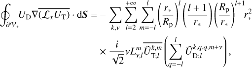 (F.8)
(F.8)

where the dependence on r* vanishes, as discussed by Ogilvie (2013). Finally, using the formula given by Eq. (57), established in Appendix C, we end up with
 (F.10)
which corresponds to Eq. (58). The expressions provided by Eqs. (59–61) for the other components of the torque and the tidal power are derived following similar steps.
Appendix G Tide-raising gravitational potential
In this appendix we derive the expression for the components of the tide-raising gravitational potential given Eq. (65). First, the tidal potential, defined by Eq. (5), is expanded as a series of Legendre polynomials (e.g. Efroimsky & Williams 2009),
 (G.1)
(G.1)
where Ψ designates the stellar zenithal angle (with Ψ = 0 at the sub-stellar point), and Pl denotes the degree-l Legendre polynomial, defined by Eq. (D.3).
Next, by applying the addition theorem for spherical harmonics (e.g. Arfken & Weber 2005, Sect. 12.8), we express Pl (cos Ψ) as
 (G.2)
(G.2)
where θs and φs represent the colatitude and longitude of the per- turber in the fixed reference frame. We proceed by rewriting  as a function of the perturber’s orbital elements. This is achieved through the use of Wigner D-functions, as introduced in Eq. (26),

which can be simplified further to
 (G.3)
(G.3)
where αs, βs, and γs are the Euler angles defining the reference frame associated with the perturber’s orbit, as provided in Eq. (63). Thus, the tide-raising gravitational potential is given by
 (G.4)
(G.4)
expressed as a function of the planet-perturber distance, rs, and true anomaly, vs.
By introducing time dependence through Hansen coefficients, as in Eq. (64), we write

which is further expressed as
 (G.5)
(G.5)
Substituting this into the expression for the tidal potential, we obtain
 (G.6)
(G.6)
where the dimensionless function  is given by
 (G.7)
(G.7)
By using the symmetry properties of spherical harmonics, Wigner D-functions (e.g. Varshalovich et al. 1988, Chapter 4), and Hansen coefficients (e.g. Hughes 1981; Laskar 2005), we find
 (G.8)
(G.8)
 (G.9)
(G.9)
 (G.10)
These relations imply that  satisfies
 (G.11)
allowing us to start the summation over k from k = 0 and group terms in pairs of complex conjugates. Consequently, the forcing tidal potential is expressed as
 (G.12)
with the spatial functions  defined as
 (G.13)
and their coefficients  given by
 (G.14)
Finally, the phase factor  from Eq. (G.7) is ignored in Eq. (G.14), as it does not affect the tidal torque or dissipated power. The mean anomaly at t = 0, 𝓜s;0, can be set to zero. In the circular orbit case (es = 0), the true anomaly equals the mean anomaly, and the Hansen coefficients simplify to
 (G.15)
Thus, the coefficients  from Eq. (G.14) become
 (G.16)
Appendix H Convergence tests for tidal solutions
The LTEs given by Eqs. (88) and (89) are solved in the frequency domain using the spectral method described in detail in Auclair- Desrotour et al. (2023). These solutions are expressed as series of spherical harmonics, which are theoretically infinite. However, to solve the problem numerically, we must truncate these series. The truncation degree, N, is chosen to ensure that the error induced by this approximation remains negligible. To determine an appropriate value for N, we performed convergence tests. In all cases, we used the simplified Earth-Moon system described in Sect. 4, considering the coplanar-circular configuration and the parameter values given by Table 1. Under this configuration, the planet is distorted solely by the semidiurnal tide, and the tidal torque is applied around the planet’s spin axis, which aligns with the total angular momentum vector. This means that 𝒯x = 0 and 𝒯y = 0. We calculated the evolution of the component 𝒯z across a uniformly sampled range of semidiurnal tidal frequencies by varying the planet’s rotation rate.
Figure H.1 presents the results for truncation degrees between N = 2 (very low resolution) and N = 60 (high resolution). The spectra display a series of peaks, as seen in Figs. 4 and 5, corresponding to the typical pattern of oceanic tidal solutions in Laplace’s theory (e.g. Auclair-Desrotour et al. 2018; Motoyama et al. 2020; Tyler 2021). Each peak arises from the resonant excitation of an oceanic surface gravity mode by the tide-raising potential. In the global, uniform-depth ocean we studied, Laplace’s tidal problem admits semi-analytical solutions, expressed as series of the so-called Hough functions. These are spherical harmonics distorted by the planet’s rotation (e.g. Longuet-Higgins 1968). Since these functions differ from  , the semidiurnal tidal potential couples with several modes. The lowest frequency peak in Fig. H.1 corresponds to the ocean mode with the largest horizontal structure, which is also closest to the
  harmonic. As the latitudinal wavelength of the resonantly excited modes decreases, the frequency of the peaks increases. Garrett & Munk (1971) provide a closed-form solution for the LTEs, offering a discussion about the dependence of oceanic tidal elevation on tidal frequency (see also Auclair- Desrotour et al. 2019, Eq. (55), for the formulation of the oceanictidal torque as a function of the tidal frequency). The peak near synchronisation (Ω = ns) corresponds to the maximum predicted by the Andrade model, which accounts for the tidal response of solid regions (see e.g. Efroimsky 2012b, Fig. 2).
As the truncation degree increases, the tidal solutions capture more resonant peaks. A truncation degree of N = 5 appears sufficient to define the main peak, while setting N = 10 captures the second peak, and so forth. It is worth noting that the dynamical ocean tide diminishes at higher tidal frequencies because the overlap between the ocean modes and the  spherical harmonic decreases. In the high-frequency range, the solution is dominated by the contribution of solid tides, which leads to a smoother evolution of the torque with the tidal frequency. Consequently, very high spectral resolutions are not required to accurately capture the planet’s tidal response. Beyond N = 30, the difference between numerical and exact solutions becomes negligible. Therefore, for practical purposes, we set N = 30, as used in the calculations in Sect. 4.
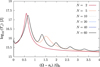 |
Fig. H.1 Semidiurnal tidal torque about the spin axis of a rocky planet with a global, uniform-depth ocean in the coplanar-circular configuration for various truncation degrees of the tidal solution ranging between N = 2 and N = 60. The torque is computed using Eq. (60). It is plotted as a function of the normalised tidal frequency, ω = (Ω − ns) /ΩE, with ΩE = 7.2921 × 10⁻⁵ rad s−1 being Earth’s actual angular velocity (Fienga et al. 2021). |
Appendix I Tidal gravitational potentials in the rotating frame of reference of the perturber
Since the tidal perturbation follows the perturber’s motion, the coordinate system in which the perturber remains fixed is the most appropriate for representing both the tidal forcing gravitational potential, UT, and the gravitational potential induced by the tidal response, UD. In this section we derive the expressions for these two potentials in the rotated coordinate system,  , where
  and
and  correspond to the sub-satellite point, while r̂ = r .It is important to note that the notations
  are also used to refer to the coordinate system associated with the planet’s rotating reference frame, which should not be confused with the frame associated with the perturber.
The gravitational tidal potential is expressed by Eq. (19) in the Galilean reference frame, ℛf: (O, ex, ey, ez), corresponding to the coordinates (r, θ, φ). Each Fourier component of this potential is expanded as a series of spherical harmonics (see Eq. (23)). Therefore, we transition from the fixed coordinate system, (r, θ, φ), to the rotated coordinate system,  , by employing the Wigner-D elements introduced in Eq. (26), as follows:
 (I.1)
(I.1)
The Euler rotation angles (αs,βs,γs) are those defined in Eq. (63). These angles specify the rotation that transitions from the Galilean reference frame to the reference frame associated with the perturber’s orbital motion.
By replacing the index m with j and the index q with m, we can rewrite Eq. (23) as
 (I.2)
(I.2)
where  now depends implicitly on time via the perturber’s true anomaly, vs. To account for this, we express the factor
  as a Fourier series using Eq. (64), yielding
 (I.3)
(I.3)
By grouping the time-dependent factors, we can identify the tidal frequencies associated with each Fourier component of the tidal potential in the perturber’s frame,  . Given that σk = kns, only a single index is needed to define these tidal frequencies. Thus, we introduce the index q = k + p, allowing us to rewrite the forcing tidal potential as
 (I.4)
(I.4)
In this expression, the spatial functions  are given by
 (I.5)
(I.5)
where the complex coefficients  are defined as
 (I.6)
(I.6)
As discussed in Appendix G, the mean anomaly at t = 0 can be set to zero, since it does not affect the tidal torque and dissipated power. Thus, the phase factor in Eq. (I.6) can be ignored.
For the components of the tidal potential UD that correspond to the same frequencies as the tidal forcing (i.e. components where p = q in Eq. (20)), similar expressions can be obtained. These are the components that contribute to the tidal power and torque, while others cannot generally couple with the forcing. Neglecting these other components, Equation (20) becomes
 (I.7)
(I.7)
where the spatial functions  are expressed as
 (I.8)
(I.8)
The complex coefficients  in the above equations are given by
 (I.9)
(I.9)
The same coordinate transformation steps as those applied to the forcing tidal potential are used to rewrite the tidal response potential as
 (I.10)


The complex coefficients  are expressed as
 (I.12)
Appendix J Sensitivities of the tidal potential and torque to ocean tides
For comparison, we computed the maps in Fig. 8 for a global ocean with rigid solid regions and repeated this analysis for deformable solid regions. The results are shown in Fig. J.1. When considering the coupled tidal response of both the solid part and ocean components, we find that the tidal potential and torque exhibit markedly different sensitivities to the oceanic tidal response. Variations in self-attraction are largely unaffected by oceanic tides. The predominant patterns in Fig. J.1 arise from the distortion of solid regions. In contrast, the tidal torque and dissipated power are heavily influenced by oceanic tides, as highlighted in Figs. 4–6. Notably, the tidal torque can be significantly amplified by the resonances of the tidally forced gravity modes, unlike the tidal potential. We elucidate this seemingly counterintuitive behaviour using a simple toy model.
We consider a coplanar-circular configuration, where the per- turber orbits the planet in a circular path within its equatorial plane. In this scenario, the only tidal component contributing to the orbital and rotational evolution of the planet-perturber system is the semidiurnal tide. Additionally, we adopt the per- turber’s reference frame introduced in Sect. 4.3, where the perturber is static, and the associated system of coordinates,  . The sub-perturber point is defined as
  . Under these assumptions, the gravitational potential induced by the tidal deformation of the body is expressed as
 (J.1)
(J.1)
where Z is a complex coefficient. In linear theory, the tidal torque scales as 𝒯z ∝ ℑ {Z} while the spatial distribution of the tidal potential scales as  , with arg Z denoting the argument of Z. Therefore, it is essential to examine how ℑ {Z}, |Z|, and argZ depend on the solid and oceanic tidal responses.
The complex coefficient Z can be decomposed as
 (J.2)
(J.2)
where Zsol and Zoc represent the contributions from solid and oceanic tides, respectively. These complex coefficients can be written as
 (J.3)
(J.3)
where αsol and αoc are the phase angles associated with each response. For simplicity, we assume that both the solid and oceanic responses experience slight delays relative to the tideraising potential, such that αsol << 1 and αoc << 1. We denote the ratio of the moduli as η = |Zoc|/|Zsol|. The real and imaginary parts of Z are given by
 (J.4)
(J.4)
 (J.5)
(J.5)
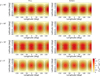 |
Fig. J.1 Gravitational potential induced by the tidal response of an ocean planet with deformable solid regions in the system of coordinates rotating with the perturber for Prot = 10 hr and obliquity values ranging between 0° and 90°. Left: maximum amplitude of the tidal potential obtained from the full calculation (FULL). Right: maximum amplitude of the tidal potential obtained with the standard approximation based on the equatorial degree-2 Love number (APPROX). Amplitudes are plotted as functions of longitude, |


Using first-order Taylor expansions in αsol and αoc, these simplify to
 (J.6)
(J.6)
 (J.7)
(J.7)
From these equations, we can deduce the modulus and argument of Z,
 (J.8)
(J.8)
 (J.9)
(J.9)
The solid tide is characterised as an equilibrium tide, meaning that αsol is very small and |Zsol| is relatively independent on tidal frequency. Conversely, the oceanic tide is highly sensitive to tidal frequency within the resonant regime, leading to significant variations in αoc. It follows that αsol << αoc. However, due to the density difference between solid rock and liquid water, η << 1 generally holds true. Consequently, |Z| remains nearly constant, and arg Z << 1, while 𝔍 {Z} ∝ αoc under the condition that αsol << ηαoc. This illustrates how the sensitivities of the tidal torque and potential to the oceanic tidal response can differ significantly.
References
- Abramowitz, M., & Stegun, I. A. 1972, Handbook of Mathematical Functions (New York: Dover) [Google Scholar]
- Alterman, Z., Jarosch, H., & Pekeris, C. L. 1959, Proc. Roy. Soc. London Ser. A, 252, 80 [NASA ADS] [CrossRef] [Google Scholar]
- Andrade, E. N. D. C. 1910, Proc. Roy. Soc. London Ser. A, 84, 1 [NASA ADS] [CrossRef] [Google Scholar]
- Arbic, B. K. 2022, Progr. Oceanogr., 206, 102824 [NASA ADS] [CrossRef] [Google Scholar]
- Arbic, B. K., & Garrett, C. 2010, Continental Shelf Res., 30, 564 [NASA ADS] [CrossRef] [Google Scholar]
- Arfken, G. B., & Weber, H. J. 2005, Mathematical Methods for Physicists, 6th ed. (Amsterdam; Boston: Elsevier) [Google Scholar]
- Astoul, A., & Barker, A. J. 2022, MNRAS, 516, 2913 [NASA ADS] [CrossRef] [Google Scholar]
- Astoul, A., & Barker, A. J. 2023, ApJ, 955, L23 [NASA ADS] [CrossRef] [Google Scholar]
- Auclair-Desrotour, P., Le Poncin-Lafitte, C., & Mathis, S. 2014, A&A, 561, L7 [NASA ADS] [CrossRef] [EDP Sciences] [Google Scholar]
- Auclair Desrotour, P., Mathis, S., & Le Poncin-Lafitte, C. 2015, A&A, 581, A118 [NASA ADS] [CrossRef] [EDP Sciences] [Google Scholar]
- Auclair-Desrotour, P., Mathis, S., Laskar, J., & Leconte, J. 2018, A&A, 615, A23 [EDP Sciences] [Google Scholar]
- Auclair-Desrotour, P., Leconte, J., Bolmont, E., & Mathis, S. 2019, A&A, 629, A132 [NASA ADS] [CrossRef] [EDP Sciences] [Google Scholar]
- Auclair-Desrotour, P., Farhat, M., Boué, G., Gastineau, M., & Laskar, J. 2023, A&A, 680, A13 [NASA ADS] [CrossRef] [EDP Sciences] [Google Scholar]
- Bartlett, B. C., & Stevenson, D. J. 2016, Geophys. Res. Lett., 43, 5716 [NASA ADS] [CrossRef] [Google Scholar]
- Baruteau, C., & Rieutord, M. 2013, J. Fluid Mech., 719, 47 [Google Scholar]
- Bell Jr, T. 1975, J. Geophys. Res., 80, 320 [NASA ADS] [CrossRef] [Google Scholar]
- Beuthe, M. 2016, Icarus, 280, 278 [CrossRef] [Google Scholar]
- Blackledge, B. W., Green, J. A. M., Barnes, R., & Way, M. J. 2020, Geophys. Res. Lett., 47, e85746 [NASA ADS] [CrossRef] [Google Scholar]
- Bolmont, E. 2018, Habitability in Brown Dwarf Systems, eds. H. J. Deeg, & J. A. Belmonte (Cham: Springer International Publishing), 1 [Google Scholar]
- Bolmont, E., Breton, S. N., Tobie, G., et al. 2020, A&A, 644, A165 [NASA ADS] [CrossRef] [EDP Sciences] [Google Scholar]
- Boué, G. 2017, Celest. Mech. Dyn. Astron., 128, 261 [CrossRef] [Google Scholar]
- Boué, G. & Efroimsky, M. 2019, Celest. Mech. Dyn. Astron., 131, 30 [CrossRef] [Google Scholar]
- Boué, G., Correia, A. C. M., & Laskar, J. 2016, Celest. Mech. Dyn. Astron., 126, 31 [CrossRef] [Google Scholar]
- Boyd, J. P. 1978, J. Atmos. Sci., 35, 2236 [NASA ADS] [CrossRef] [Google Scholar]
- Bretherton, F. P. 1969, Q. J. Roy. Meteorol. Soc., 95, 754 [NASA ADS] [CrossRef] [Google Scholar]
- Brian K. Arbic, R. H. K., & Garrett, C. 2009, Atmosphere-Ocean, 47, 239 [NASA ADS] [CrossRef] [Google Scholar]
- Cartwright, D. E. 1977, Rep. Progr. Phys., 40, 665 [CrossRef] [Google Scholar]
- Castelnau, O., Duval, P., Montagnat, M., & Brenner, R. 2008, J. Geophys. Res. (Solid Earth), 113, B11203 [NASA ADS] [CrossRef] [Google Scholar]
- Castillo-Rogez, J. C., Efroimsky, M., & Lainey, V. 2011, J. Geophys. Res. (Planets), 116, E09008 [CrossRef] [Google Scholar]
- Chen, E. M. A., Nimmo, F., & Glatzmaier, G. A. 2014, Icarus, 229, 11 [NASA ADS] [CrossRef] [Google Scholar]
- Correia, A. C. M., & Laskar, J. 2001, Nature, 411, 767 [Google Scholar]
- Correia, A. C. M., & Laskar, J. 2003, J. Geophys. Res. (Planets), 108, 5123 [NASA ADS] [CrossRef] [Google Scholar]
- Correia, A. C. M., & Valente, E. F. S. 2022, Celest. Mech. Dyn. Astron., 134, 24 [NASA ADS] [CrossRef] [Google Scholar]
- Daher, H., Arbic, B. K., Williams, J. G., et al. 2021, J. Geophys. Res. (Planets), 126, e06875 [NASA ADS] [Google Scholar]
- Efroimsky, M. 2012a, Celest. Mech. Dyn. Astron., 112, 283 [NASA ADS] [CrossRef] [Google Scholar]
- Efroimsky, M. 2012b, ApJ, 746, 150 [Google Scholar]
- Efroimsky, M., & Lainey, V. 2007, J. Geophys. Res. (Planets), 112, E12003 [NASA ADS] [CrossRef] [Google Scholar]
- Efroimsky, M., & Williams, J. G. 2009, Celest. Mech. Dyn. Astron., 104, 257 [NASA ADS] [CrossRef] [Google Scholar]
- Egbert, G. D., & Ray, R. D. 2000, Nature, 405, 775 [NASA ADS] [CrossRef] [Google Scholar]
- Egbert, G. D., & Ray, R. D. 2001, J. Geophys. Res., 106, 22 [Google Scholar]
- Egbert, G. D., & Ray, R. D. 2003, Geophys. Res. Lett., 30, 1907 [NASA ADS] [CrossRef] [Google Scholar]
- Egbert, G. D., Ray, R. D., & Bills, B. G. 2004, J. Geophys. Res. (Oceans), 109, C03003 [CrossRef] [Google Scholar]
- Farhat, M., Auclair-Desrotour, P., Boué, G., & Laskar, J. 2022a, A&A, 665, L1 [NASA ADS] [CrossRef] [EDP Sciences] [Google Scholar]
- Farhat, M., Laskar, J., & Boué, G. 2022b, J. Geophys. Res. (Solid Earth), 127, e2021JB023323 [NASA ADS] [CrossRef] [Google Scholar]
- Farhat, M., Auclair-Desrotour, P., Boué, G., Deitrick, R., & Laskar, J. 2024, A&A, 684, A49 [NASA ADS] [CrossRef] [EDP Sciences] [Google Scholar]
- Fienga, A., Deram, P., Di Ruscio, A., et al. 2021, Notes Scientifiques et Techniques de l’Institut de Mecanique Celeste, 110 [Google Scholar]
- Fuller, J., Guillot, T., Mathis, S., & Murray, C. 2024, Space Sci. Rev., 220, 22 [CrossRef] [Google Scholar]
- Garrett, C., & Kunze, E. 2007, Annu. Rev. Fluid Mech., 39, 57 [NASA ADS] [CrossRef] [Google Scholar]
- Garrett, C.J. R., & Munk, W. H. 1971, Deep Sea Res. A, 18, 493 [NASA ADS] [Google Scholar]
- Gastineau, M., & Laskar, J. 2011, ACM Commun. Comput. Algebra, 44, 194 [Google Scholar]
- Gerkema, T. 2019, An Introduction to Tides (Cambridge University Press) [CrossRef] [Google Scholar]
- Gerkema, T., Zimmerman, J. T. F., Maas, L. R. M., & van Haren, H. 2008, Rev. Geophys., 46, RG2004 [Google Scholar]
- Gimbutas, Z., & Greengard, L. 2009, J. Computat. Phys., 228, 5621 [NASA ADS] [CrossRef] [Google Scholar]
- Gold, T., & Soter, S. 1969, Icarus, 11, 356 [NASA ADS] [CrossRef] [Google Scholar]
- Goldreich, P., & Soter, S. 1966, Icarus, 5, 375 [Google Scholar]
- Green, J. A. M., Huber, M., Waltham, D., Buzan, J., & Wells, M. 2017, Earth Planet. Sci. Lett., 461, 46 [CrossRef] [Google Scholar]
- Guenel, M., Baruteau, C., Mathis, S., & Rieutord, M. 2016, A&A, 589, A22 [NASA ADS] [CrossRef] [EDP Sciences] [Google Scholar]
- Hay, H. C. F. C., & Matsuyama, I. 2019, Icarus, 319, 68 [NASA ADS] [CrossRef] [Google Scholar]
- Hendershott, M. C. 1972, Geophys. J., 29, 389 [NASA ADS] [CrossRef] [Google Scholar]
- Henning, W. G., O’Connell, R. J., & Sasselov, D. D. 2009, ApJ, 707, 1000 [Google Scholar]
- Hough, S. S. 1898, Roy. Soc. London Philos. Trans. Ser. A, 191, 139 [NASA ADS] [CrossRef] [Google Scholar]
- Huang, H., Ma, C., Laskar, J., et al. 2024, PNAS, 121, e2317051121 [NASA ADS] [CrossRef] [Google Scholar]
- Hughes, S. 1981, Celest. Mech., 25, 101 [NASA ADS] [CrossRef] [Google Scholar]
- Hut, P. 1980, A&A, 92, 167 [NASA ADS] [Google Scholar]
- Hut, P. 1981, A&A, 99, 126 [NASA ADS] [Google Scholar]
- Ingersoll, A. P., & Dobrovolskis, A. R. 1978, Nature, 275, 37 [CrossRef] [Google Scholar]
- Jayne, S. R., & St. Laurent, L. C. 2001, Geophys. Res. Lett., 28, 811 [NASA ADS] [CrossRef] [Google Scholar]
- Kamata, S., Matsuyama, I., & Nimmo, F. 2015, J. Geophys. Res. (Planets), 120, 1528 [NASA ADS] [CrossRef] [Google Scholar]
- Karato, S., & Spetzler, H. A. 1990, Rev. Geophys., 28, 399 [CrossRef] [Google Scholar]
- Kaula, W. M. 1964, Rev. Geophys. Space Phys., 2, 661 [Google Scholar]
- Laplace, P. S. 1798, Traité de mécanique céleste (Duprat J. B. M.) [Google Scholar]
- Laskar, J. 2005, Celest. Mech. Dyn. Astron., 91, 351 [NASA ADS] [CrossRef] [Google Scholar]
- Laskar, J., Farhat, M., Lantink, M. L., et al. 2024, Sedimentologika, 2, 1271 [NASA ADS] [CrossRef] [Google Scholar]
- Leconte, J., Wu, H., Menou, K., & Murray, N. 2015, Science, 347, 632 [NASA ADS] [CrossRef] [Google Scholar]
- Lee, U., & Saio, H. 1997, ApJ, 491, 839 [Google Scholar]
- Lindzen, R. S., & Blake, D. 1972, J. Geophys. Res., 77, 2166 [NASA ADS] [CrossRef] [Google Scholar]
- Lindzen, R. S., & Chapman, S. 1969, Space Sci. Rev., 10, 3 [NASA ADS] [CrossRef] [Google Scholar]
- Longuet-Higgins, M. S. 1968, Philos. Trans. Roy. Soc. London Ser. A, 262, 511 [NASA ADS] [CrossRef] [Google Scholar]
- Lyard, F. H., Allain, D. J., Cancet, M., Carrère, L., & Picot, N. 2021, Ocean Sci., 17, 615 [NASA ADS] [CrossRef] [Google Scholar]
- MacDonald, G. J. F. 1964, Rev. Geophys. Space Phys., 2, 467 [Google Scholar]
- Mathis, S., Le Poncin-Lafitte, C., & Remus, F. 2013, in Lecture Notes in Physics, Berlin Springer Verlag, 861, eds. J. Souchay, S. Mathis, & T. Tokieda, 255 [NASA ADS] [CrossRef] [Google Scholar]
- Mathis, S., Auclair-Desrotour, P., Guenel, M., Gallet, F., & Le Poncin-Lafitte, C. 2016, A&A, 592, A33 [NASA ADS] [CrossRef] [EDP Sciences] [Google Scholar]
- Matsuyama, I. 2014, Icarus, 242, 11 [NASA ADS] [CrossRef] [Google Scholar]
- Matsuyama, I., Beuthe, M., Hay, H. C. F. C., Nimmo, F., & Kamata, S. 2018, Icarus, 312, 208 [NASA ADS] [CrossRef] [Google Scholar]
- Mitchell, R. N., & Kirscher, U. 2023, Nat. Geosci., 16, 567 [NASA ADS] [CrossRef] [Google Scholar]
- Motoyama, M., Tsunakawa, H., & Takahashi, F. 2020, Icarus, 335, 113382 [NASA ADS] [CrossRef] [Google Scholar]
- Munk, W. H., & MacDonald, G. J. F. 1960, The rotation of the earth; a geophysical discussion (New York: Cambridge University Press) [Google Scholar]
- Ogilvie, G. I. 2009, MNRAS, 396, 794 [Google Scholar]
- Ogilvie, G. I. 2013, MNRAS, 429, 613 [Google Scholar]
- Ogilvie, G. I. 2014, ARA&A, 52, 171 [Google Scholar]
- Ogilvie, G. I., & Lin, D. N. C. 2004, ApJ, 610, 477 [Google Scholar]
- Ogilvie, G. I., & Lin, D. N. C. 2007, ApJ, 661, 1180 [Google Scholar]
- Ortland, D. A. 2005a, J. Atmos. Sci., 62, 2684 [NASA ADS] [CrossRef] [Google Scholar]
- Ortland, D. A. 2005b, J. Atmos. Sci., 62, 2674 [NASA ADS] [CrossRef] [Google Scholar]
- Peale, S. J. 2003, Celest. Mech. Dyn. Astron., 87, 129 [CrossRef] [Google Scholar]
- Peale, S. J., Cassen, P., & Reynolds, R. T. 1979, Science, 203, 892 [Google Scholar]
- Peltier, W. R. 1974, Rev. Geophys. Space Phys., 12, 649 [CrossRef] [Google Scholar]
- Ray, R. D. 1998, Mar. Geodesy, 21, 181 [NASA ADS] [CrossRef] [Google Scholar]
- Ray, R. D., Eanes, R. J., Egbert, G. D., & Pavlis, N. K. 2001, Geophys. Res. Lett., 28, 21 [NASA ADS] [CrossRef] [Google Scholar]
- Rekier, J., Trinh, A., Triana, S. A., & Dehant, V. 2019, J. Geophys. Res. (Planets), 124, 2198 [NASA ADS] [CrossRef] [Google Scholar]
- Rieutord, M. 2015, Fluid Dynamics: An Introduction (Springer) [Google Scholar]
- Rovira-Navarro, M., Matsuyama, I., & Hay, H. C. F. C. 2023, Planetary Science Journal, 4, 23 [CrossRef] [Google Scholar]
- Rubincam, D. P. 2016, Icarus, 266, 24 [NASA ADS] [CrossRef] [Google Scholar]
- Savonije, G. J., & Witte, M. G. 2002, A&A, 386, 211 [NASA ADS] [CrossRef] [EDP Sciences] [Google Scholar]
- Sotin, C., Grasset, O., & Mocquet, A. 2007, Icarus, 191, 337 [Google Scholar]
- Takeuchi, H., & Saito, M. 1972, Methods Computat. Phys., 11, 217 [Google Scholar]
- Tiesinga, E., Mohr, P. J., Newell, D. B., & Taylor, B. N. 2021, J. Phys. Chem. Ref. Data, 50, 033105 [NASA ADS] [CrossRef] [Google Scholar]
- Tobie, G., Mocquet, A., & Sotin, C. 2005, Icarus, 177, 534 [Google Scholar]
- Tremaine, S., Touma, J., & Namouni, F. 2009, AJ, 137, 3706 [Google Scholar]
- Tyler, R. H. 2008, Nature, 456, 770 [NASA ADS] [CrossRef] [Google Scholar]
- Tyler, R. H. 2009, Geophys. Res. Lett., 36, L15205 [Google Scholar]
- Tyler, R. 2011, Icarus, 211, 770 [NASA ADS] [CrossRef] [Google Scholar]
- Tyler, R. 2014, Icarus, 243, 358 [NASA ADS] [CrossRef] [Google Scholar]
- Tyler, R. H. 2020, Icarus, 348, 113821 [NASA ADS] [CrossRef] [Google Scholar]
- Tyler, R. H. 2021, Planetary Science Journal, 2, 70 [CrossRef] [Google Scholar]
- Valente, E. F. S., & Correia, A. C. M. 2022, A&A, 665, A130 [NASA ADS] [CrossRef] [EDP Sciences] [Google Scholar]
- Vallis, G. K. 2006, Atmospheric and Oceanic Fluid Dynamics (Cambridge University Press), 770 [Google Scholar]
- Varshalovich, D. A., Moskalev, A. N., & Khersonskii, V. K. 1988, Quantum Theory of Angular Momentum (World Scientific Publishing Company) [CrossRef] [Google Scholar]
- Wang, H., Boyd, J. P., & Akmaev, R. A. 2016, Geosci. Model Dev., 9, 1477 [Google Scholar]
- Webb, D. J. 1980, Geophys. J., 61, 573 [NASA ADS] [CrossRef] [Google Scholar]
- Wilmes, S. B., Pedersen, V. K., Schindelegger, M., & Green, J. A. M. 2023, Paleoceanogr. Paleoclimatol., 38, e2023PA004727 [NASA ADS] [CrossRef] [Google Scholar]
- Wu, H., Murray, N., Menou, K., Lee, C., & Leconte, J. 2023, Sci. Adv., 9, eadd2499 [NASA ADS] [CrossRef] [Google Scholar]
- Wu, Y., Malinverno, A., Meyers, S. R., & Hinnov, L. A. 2024, Sci. Adv., 10, eado2412 [NASA ADS] [CrossRef] [Google Scholar]
- Zahn, J. P. 1966, Ann. Astrophys., 29, 313 [NASA ADS] [Google Scholar]
- Zahn, J.-P. 1975, A&A, 41, 329 [Google Scholar]
- Zahnle, K., & Walker, J. C. G. 1987, Precamb. Res., 37, 95 [NASA ADS] [CrossRef] [Google Scholar]
- Zhou, M., Wu, H., Hinnov, L. A., et al. 2024, Sci. Adv., 10, eadn7674 [NASA ADS] [CrossRef] [Google Scholar]
The potential Love number should not be confused with the realvalued Love number accounting for the elastic elongation of the primary in the context of bodily tide theory, which is commonly used in the literature (e.g. Munk & MacDonald 1960; Mathis et al. 2013). By definition, this real-valued Love number is independent of dissipative processes. Therefore, it has to be complemented by the so-called tidal quality factor, usually denoted by Q, to describe the action of tides on the longterm evolution of planetary systems (e.g. MacDonald 1964; Goldreich & Soter 1966; Efroimsky & Williams 2009). As the complex-valued Love number used here relies on a more general definition of the tidal response, this transfer function appears to be more suited to the study of fluid tides than the elastic Love number, and the term ‘Love number’ thus systematically refers to it throughout the article.
Tides are low-frequency disturbances relative to the vibrational (or seismic) modes of rocky bodies, which prevents these modes from being resonantly excited by tidal forces. For example, the typical periods of solid Earth’s free oscillations are shorter than one hour (e.g. Alterman et al. 1959).
The summation in Eq. (19) may also be defined with k running from −∞ to +∞ (see e.g. Ogilvie 2014, Eq. (3)). In that case, the spherical harmonic orders in Eqs. (23) and (24) are positive, while they range from −l to l in the present work.
Equations (72) and (75) of Auclair-Desrotour et al. (2023) contain a typo that we correct here: a missing g factor in the numerator of the second term on the right-hand side. This factor is included in the corrected formula given by Eq. (92).
Equation (E.7) is obtained by combining the recursion relations given by Eqs. (14) and (15) of Varshalovich et al. (1988), Sect. 4.8.2.
All Tables
Features of the global ocean modes that are resonantly excited by the semidiurnal tidal forces.
All Figures
|
Fig. 1 Euler angles (α, β, γ) corresponding to the 3-2-3 Euler rotation matrix defined by Eq. (1), which describes the change of coordinate systems 𝓡f : O, ex, ey, ez → 𝓡: (O, eX, eY, eZ). |
| In the text | |
|
Fig. 2 Diagram illustrating the domain 𝒱∗, which includes the central body while excluding the perturber. |
| In the text | |
|
Fig. 3 Frame of reference ℛs: (O, Is, Js, Ks) and Keplerian elements describing the orbit of the perturber. |
| In the text | |
|
Fig. 4 Tidally dissipated power (𝒫diss) as a function of the planet’s spin rotation period (horizontal axis) and obliquity (vertical axis) for Earth-sized dry (left panels) and global-ocean (right panels) planets. Top: full calculation of the planet’s tidal response (FULL). Middle: calculation using, for all tidal forcing terms, the degree-2 Love number computed in the equatorial plane assuming the coplanar-circular configuration (APPROX). Bottom: relative difference between the FULL and APPROX cases, defined by Eq. (93). The tidally dissipated power was computed from the tidal power and torque using Eq. (81). The dashed green lines indicate the resonances associated with the oceanic surface gravity modes (see Eq. (95) and Table 2), and the dashed magenta lines the 1:1 and 2:1 spin-orbit resonances. The black dot at (Prot, β) = (1 day, 0°) designates the actual Earth-Moon system in the coplanar-circular approximation. |
| In the text | |
|
Fig. 5 Variation rate of the planet’s spin angular velocity (Ω) as a function of the planet’s spin rotation period (horizontal axis) and obliquity (vertical axis) for Earth-sized dry (left panels) and global-ocean (right panels) planets. Top: full calculation of the planet’s tidal response (FULL). Middle: calculation using, for all tidal forcing terms, the degree-2 Love number computed in the equatorial plane assuming the coplanar-circular configuration (APPROX). Bottom: relative difference between the FULL and APPROX cases, defined by Eq. (93). The variation rate of the planet’s spin angular velocity was computed from the three-dimensional tidal torque using Eq. (75). The black dot at (Prot,β) = (1 day, 0°) designates the actual Earth-Moon system in the coplanar-circular approximation. |
| In the text | |
|
Fig. 6 Variation rate of the planet’s obliquity |
| In the text | |
|
Fig. 7 Gravitational potential induced by the tidal response of an ocean planet with rigid solid regions in the system of coordinates rotating with the perturber for Prot = 33 h and obliquity values ranging between 0° and 90°. Left: maximum amplitude of the tidal potential obtained from the full calculation (FULL). Right: maximum amplitude of the tidal potential obtained with the standard approximation based on the equatorial degree-2 Love number (APPROX). Amplitudes are plotted as functions of longitude, |
| In the text | |
|
Fig. 8 Gravitational potential induced by the tidal response of an ocean planet with rigid solid regions in the system of coordinates rotating with the perturber for Prot = 10 h and obliquity values ranging between 0° and 90°. Left: maximum amplitude of the tidal potential obtained from the full calculation (FULL). Right: maximum amplitude of the tidal potential obtained with the standard approximation based on the equatorial degree-2 Love number (APPROX). Amplitudes are plotted as functions of longitude, |
| In the text | |
|
Fig. H.1 Semidiurnal tidal torque about the spin axis of a rocky planet with a global, uniform-depth ocean in the coplanar-circular configuration for various truncation degrees of the tidal solution ranging between N = 2 and N = 60. The torque is computed using Eq. (60). It is plotted as a function of the normalised tidal frequency, ω = (Ω − ns) /ΩE, with ΩE = 7.2921 × 10⁻⁵ rad s−1 being Earth’s actual angular velocity (Fienga et al. 2021). |
| In the text | |
|
Fig. J.1 Gravitational potential induced by the tidal response of an ocean planet with deformable solid regions in the system of coordinates rotating with the perturber for Prot = 10 hr and obliquity values ranging between 0° and 90°. Left: maximum amplitude of the tidal potential obtained from the full calculation (FULL). Right: maximum amplitude of the tidal potential obtained with the standard approximation based on the equatorial degree-2 Love number (APPROX). Amplitudes are plotted as functions of longitude, |
| In the text | |
Current usage metrics show cumulative count of Article Views (full-text article views including HTML views, PDF and ePub downloads, according to the available data) and Abstracts Views on Vision4Press platform.
Data correspond to usage on the plateform after 2015. The current usage metrics is available 48-96 hours after online publication and is updated daily on week days.
Initial download of the metrics may take a while.