| Issue |
A&A
Volume 693, January 2025
|
|
|---|---|---|
| Article Number | A248 | |
| Number of page(s) | 14 | |
| Section | Extragalactic astronomy | |
| DOI | https://doi.org/10.1051/0004-6361/202452556 | |
| Published online | 21 January 2025 | |
Exploring the dark matter disk model in dwarf galaxies: Insights from the LITTLE THINGS sample
1
Centro Ricerche Enrico Fermi, I-00184 Roma, Italy
2
INFN Unità Roma 1, Dipartimento di Fisica, Università di Roma Sapienza, I-00185 Roma, Italy
3
Dipartimento di Fisica, Sapienza, Università di Roma, I-00185 Roma, Italy
4
Complexity Science Hub Vienna, Josefstaedter Strasse 39, 1080 Vienna, Austria
5
University of Konstanz, Universitätstraße 10, 78457 Konstanz, Germany
6
Sony CSL – Rome, Joint Initiative CREF-SONY, 00184 Roma, Italy
⋆ Corresponding author; sylos@cref.it
Received:
10
October
2024
Accepted:
11
December
2024
We conducted an analysis of the velocity field of dwarf galaxies in the sample collected by the Local Irregulars That Trace Luminosity Extremes and The H I Nearby Galaxy Survey (LITTLE THINGS) and focused on deriving 2D velocity maps that encompass the transverse and radial velocity fields. Within the range of radial distances in which velocity anisotropies are sufficiently small for the disk to be considered supported by rotation and where the warped geometry of the disk can be neglected, we reconstructed the rotation curve while taking the effect of the asymmetric drift into account. To fit the rotation curves, we employed the standard halo model and the dark matter disk (DMD) model, which assumes that dark matter is primarily confined to the galactic disks and can be traced by the distribution of H I. Interestingly, our analysis revealed that the fits from the DMD model are statistically comparable to those obtained using the standard halo model, but the inferred masses of the galaxies in the DMD model are approximately 10 to 100 times lower than the masses inferred in the standard halo model. In the DMD model, the inner slope of the rotation curve is directly related to a linear combination of the surface density profiles of the stellar and gas components, which generally exhibit a flat core. Consequently, the observation of a linear relation between the rotation curve and the radius in the central disk regions is consistent with the framework of the DMD model.
Key words: galaxies: dwarf / galaxies: general / galaxies: halos / galaxies: kinematics and dynamics / galaxies: structure
© The Authors 2025
 Open Access article, published by EDP Sciences, under the terms of the Creative Commons Attribution License (https://creativecommons.org/licenses/by/4.0), which permits unrestricted use, distribution, and reproduction in any medium, provided the original work is properly cited.
This article is published in open access under the Subscribe to Open model. Subscribe to A&A to support open access publication.
1. Introduction
In recent decades, the study of neutral hydrogen (H I) using high-resolution radio interferometric surveys has greatly advanced our understanding of the kinematic properties of galaxies. Two notable surveys, The H I Nearby Galaxy Survey (THINGS; Walter et al. 2008) and the Local Irregulars That Trace Luminosity Extremes (THINGS) (LITTLE THINGS; Hunter et al. 2012), have been instrumental in this field. These surveys have provided us with the means to measure high-resolution H I rotation curves, which are crucial for unravelling the mass distributions of galaxies.
The THINGS sample of galaxies was selected to encompass a wide range of physical properties spanning from low-mass metal-poor quiescent dwarf galaxies to massive spiral galaxies. In contrast, the LITTLE THINGS sample primarily consists of late-type dwarf galaxies. These dwarf galaxies show a relatively simple structure and lack prominent bulge and spiral components. Consequently, they offer a valuable opportunity to study the distribution and quantity of dark matter (DM) since this mass component significantly influences their dynamics. The H I observations from these surveys have provided substantial observational constraints on the central distribution of DM in galaxies.
Motivated by cosmological simulations, the commonly adopted assumption is that disk galaxies are quasi-flattened systems that are primarily governed by rotation and are surrounded by nearly spherical halos with an almost isotropic velocity dispersion. Various halo models have been employed to interpret the observed kinematic properties of these galaxies. The standard model is the Navarro-Frenk-White (NFW) model (Navarro et al. 1996) that was found to satisfactorily describe nonlinear structures emerging from cosmological Λ cold dark matter (ΛCDM) simulations. The NFW model is commonly referred to as a cusp-like halo model because it assumes a density power-law behavior, ρ(r)∼rα with α ≈ −1, in the central region of the halos (Moore 1994; Navarro et al. 1996, 1997, 2004, 2010; Moore et al. 1999; Power et al. 2003; Diemand et al. 2008; Stadel et al. 2009; Ishiyama et al. 2013). A core-like halo model with an almost constant density ρ(r)∼ρ0 for low values of r has also been considered in the analysis of the observed rotation curves (see, e.g., Begeman et al. 1991; Oh et al. 2015; Mancera Piña et al. 2022).
The understanding of the behavior of the density distribution in the central regions of dwarf galaxies depends on the ability to infer different DM distributions by studying their rotation curves. In many cases, these rotation curves even increase linearly in the circular velocity toward their centers, that is, vc ∝ r for low values of r, indicating a flat core in the mass density (Moore 1994; de Blok et al. 1996, 2001; de Blok & Bosma 2002; Oh et al. 2008, 2011). This clear diskrepancy between the central DM distribution within 1 kpc in galaxies observed in ΛCDM simulations and observations, known as the cusp/core problem, is one aspect that contributed to the small-scale crisis in ΛCDM cosmology (see, e.g., Kroupa 2012; Pawlowski & Kroupa 2013; Dabringhausen & Kroupa 2013). The cusps are a fundamental feature of current cosmological simulations and were repeatedly confirmed by significant increases in resolution and computing power over the years. The origin of the cusp is tied to the physical processes underlying the formation of nonlinear structures. The density profile of halo structures is characterized by a cusp in the inner regions (∼r−1) and a slower decay in the outer regions (∼r−3). It emerges from a bottom-up aggregation process. In this scenario, nonlinear structures form hierarchically through a gradual dynamical process. In contrast, when nonlinear structures form via top-down monolithic collapse, the inner region tends to exhibit a nearly flat core (Benhaiem et al. 2019; Sylos Labini et al. 2020).
Thus, in principle, the distinction between a cored profile and one with a cusp is crucial because it may indicate fundamentally different underlying dynamical evolution processes. However, this distinction becomes less clear when additional physical effects are considered in simulations. For instance, Read et al. (2016) demonstrated that stellar feedback can heat DM, resulting in a coreNFW density profile. The authors concluded that when standard cosmological simulations account for this feedback, they match the rotation curves of dwarf galaxies very well. Similarly, Lazar et al. (2020) showed that by incorporating galaxy formation physics, DM halos would exhibit density profiles that are cored and cuspy. For this reason, they introduced the core-Einasto profile, a three-parameter density model, to characterize DM halos better.
These cored profiles were used to fit galaxy rotation curves. For instance, Ou et al. (2024) fit the Milky Way rotation curve using two different mass models for the DM halo: a generalized NFW profile, and an Einasto profile (Einasto 1965; Retana-Montenegro et al. 2012). Both models included an additional free parameter compared to the standard NFW profile, which made them more suitable for fitting a declining rotation curve such as that of our own Galaxy (Eilers et al. 2019; Wang et al. 2023; Ou et al. 2024).
To measure the rotation curves of dwarf galaxies at small radii, Oh et al. (2008, 2011) used high-resolution DM density profiles of seven dwarf galaxies from the THINGS survey, supplemented with data from the Spitzer Infrared Nearby Galaxies Survey (SINGS) by Kennicutt et al. (2003). These studies showed that the average inner density slope for these galaxies is approximately α = −0.29 ± 0.07, which is consistent with the value α = −0.2 ± 0.2 derived earlier for a larger number of low surface brightness (LSB) galaxies by de Blok & Bosma (2002). This significant observational data set provides strong empirical evidence in support of the existence of a core-like distribution of DM around the centers of irregular dwarf galaxies.
To overcome the limitation in the number of galaxies probed by the THINGS survey, Oh et al. (2015) expanded the investigation by including a larger sample of dwarf galaxies. This was done by the use of data from the LITTLE THINGS survey (Hunter et al. 2012), which contains 41 nearby gas-rich dwarf galaxies that were observed with the NRAO261 very large array. The LITTLE THINGS observations have a fine angular resolution of approximately 6″ and a fine velocity resolution lower than or equal to 2.6 km s−1. In the catalog, these high-resolution observations were complemented with data in various other wavelength bands, including Hα, the optical (U, B, V), near-infrared, archival Spitzer2 infrared, and Galaxy Evolution Explorer (GALEX) ultraviolet images (Hunter & Elmegreen 2006). Follow-up observations were also conducted using ALMA and Herschel.
The availability of these high-quality multi-wavelength datasets significantly reduced observational uncertainties, which could have concealed central cusps in low-resolution data. From the initial sample of 41 galaxies, Oh et al. (2015) selected a subset of 26 dwarf galaxies (3 of which were also part of THINGS) that exhibited regular rotation patterns in their velocity fields. They measured the rotation curves using the rotating tilted-ring model (TRM; Warner et al. 1973; Rogstad et al. 1974) that distinguishes the contribution from baryons and DM. This decomposition allowed them to estimate the relative contributions to the total mass budget.
The majority of galaxies in the LITTLE THINGS sample display rotation curves that increase linearly with radius in their inner regions. The average value of the density slopes for these 26 LITTLE THINGS dwarf galaxies was found to be α = −0.32 ± 0.24, which is consistent with previous findings for low surface brightness galaxies and for the 7 THINGS dwarf galaxies. This result significantly deviates from the predicted cusp-like DM distribution (α ≃ −1) and indicates a mass distribution that is different from a cuspy distribution.
Similar results were also obtained by Iorio et al. (2017), who analyzed a subsample of 17 galaxies from the LITTLE THINGS survey. They directly fit 3D models (two spatial dimensions and one spectral dimension) using the software 3DBAROLO (Di Teodoro & Fraternali 2015). This code is based on the TRM approach that performs full 3D numerical minimization on the entire data cube. A key advantage of this approach is that the data cube models are convolved with the instrumental response, ensuring that the final results are not affected by beam smearing. The resulting rotation curves are consistent with those of Oh et al. (2015) within the errors for half of the sample galaxies. The observed differences are primarily due to variations in the best-fitting orientation angles and/or to discrepancies in the asymmetric-drift correction terms.
More recently, Mancera Piña et al. (2022) investigated how significantly mass models are affected when the possibly flared geometry of gas disks is taken into account. Accurate computations of scale heights require detailed kinematic modeling of interferometric H I and CO data, along with a robust bulge-disk decomposition. The authors found that the effect of gas flaring on the rotation curve decomposition may play a role only in the smallest gas-dominated dwarf galaxies. For most galaxies, however, the effect is minor and can safely be ignored.
In this study, we examine the LITTLE THINGS survey to estimate the mass of galaxies by employing a disk-based model for the distribution of dark matter (DM), in contrast to the standard assumption of a spherical halo DM distribution. This modeling strategy is inspired by evidence suggesting a correlation between DM and the distribution of H I gas in disk galaxies (Bosma 1978, 1981). Previous investigations of nearby disk galaxies have revealed that the ratio of the total surface density of the disk (derived from rotation curve measurements) to the surface density of gas alone (obtained from H I observational data) remains relatively constant beyond approximately one-third of the optical radius. This correlation between DM and gas in disk galaxies implies that rotation curves at larger radii may be scaled versions of those determined from the H I distribution. Several studies have indicated that the gas surface density can effectively represent the distribution of DM in galaxies. For example, Sancisi (1999), Hoekstra et al. (2001), Hessman & Ziebart (2011), Swaters et al. (2012) explored the DM-H I relation. We recall within the framework of the Bosma effect, Pfenniger et al. (1994) proposed the idea that DM might reside in the galactic disk in the form of very cold molecular hydrogen (H2). In the Milky Way, extensive clouds of cold dust (i.e., T ≈ 10 − 20 K) and dark gas, which is invisible in H I and CO, but is detected via γ-rays, were observed in the solar neighborhood by Grenier et al. (2005). Dark gas was also found by the Planck mission (Planck Collaboration XIX 2011; Casandjian et al. 2022). However, H2 in less excited and colder regions than are traced by CO has yet to be directly inferred because below 20 K, the CO molecules freeze onto dust grains, which prevents them from emitting rotational lines. Nonetheless, regions colder than 20 K are not uncommon, which means that undetected H2 may lie in the outer gas disks of galaxies, where stellar radiation decreases rapidly. Unfortunately, the direct detection of these clouds in the outer disks of galaxies remains a challenging observational task (Combes & Pfenniger 1997). Recently, Sylos Labini et al. (2024) diskovered that the rotation curves of 16 nearby disk galaxies in the THINGS sample can be accurately described by the NFW halo model and the DMD model with similar levels of precision. Furthermore, Sylos Labini et al. (2023a) demonstrated that the rotation curve of the Milky Way can be effectively modeled using the DMD. While the presence of a correlation does not imply causation, its identification may be associated with a fundamental characteristic of disk galaxies, such as the distribution of DM within the disk itself, rather than in a spherical halo that encompasses the galaxy, as is commonly assumed but not definitively proven. Therefore, it is valuable to conduct a more comprehensive investigation of this phenomenon than was undertaken previously by extending the findings of Sylos Labini et al. (2024) regarding the galaxies in the THINGS sample to the dwarf galaxies in the LITTLE THINGS sample.
To fit the DMD properly, we created our own estimation of the rotation curves for the galaxies in the LITTLE THINGS sample. For this purpose, we used the velocity ring model (VRM), as recently introduced by Sylos Labini et al. (2023b). This method operates under the assumption that the galactic disk is flat, meaning it is not warped, and it facilitates the reconstruction of coarse-grained 2D velocity maps that cover the transversal and radial velocity fields. The assumption of a flat disk generally holds true in the inner regions of galactic disks, which are the focus of our study. Warps were directly observed in the outer regions of edge-on disk galaxies (Sancisi 1976; Reshetnikov & Combes 1998; Schwarzkopf & Dettmar 2001; García-Ruiz et al. 2002; Sánchez-Saavedra et al. 2003) and typically first emerge at the optical radius. Therefore, these maps enable the examination of spatial anisotropies in the 2D velocity field within the inner disk and allow for the quantification of velocity anisotropies.
It is important to stress that the TRM and the VRM are based on two distinct assumptions. The TRM, in its simplest implementation, assumes the radial velocity to be zero, that is, vR = 0, while allowing for a warped disk geometry, whereas the VRM assumes a flat disk and permits vR ≠ 0. We adopted the VRM in this study because it enabled us to reconstruct coarse-grained 2D velocity component maps, which in turn allow for the characterization of spatial anisotropies. This approach is particularly suitable for the dwarf galaxies in the LITTLE THINGS sample because they exhibit anisotropic 2D line-of-sight velocity maps that are difficult to reconcile with a symmetric geometric deformation of the disk, such as a warp. In addition, this choice is justified a posteriori by the observation that the results for the transverse velocity obtained with the VRM are very similar to the rotation velocity derived using the TRM. Additionally, the warps in these galaxies are generally small, as indicated by the limited variation in orientation angles. This arises because dwarf galaxies, which make up our sample, have relatively limited spatial extents. Warps typically originate in tidal interactions with neighboring galaxies, and they are therefore more commonly found in the outermost regions of large disk galaxies.
The paper is structured as follows: In Sect. 2 we provide an overview of the main characteristics of the galaxies included in the LITTLE THINGS survey, which form the focus of our study. Section 3 introduces the methods we used to estimate the rotation curves of our sample galaxies and to correct for the effects of asymmetric drift. In Sect. 4 we discuss the DMD mass model we employed in our analysis. Section 5 presents and discusses the results for specific galaxies in our sample, including their rotation curves and other relevant findings. The results for the remaining galaxies are provided in Appendix C. In Sect. 6 we analyze the results of the fits using the two mass models considered in this study. Finally, Sect. 7 summarizes the main conclusions we derived from our analysis.
2. Sample
The LITTLE THINGS survey comprises 37 dwarf irregular and four blue compact dwarf galaxies known to contain H I. The distances of these nearby galaxies range from 1 Mpc to 10 Mpc, as listed in Table 1 of Hunter et al. (2012), and they exhibit a wide range of properties. More information about the galaxies included in the LITTLE THINGS sample can be found in Hunter et al. (2012), Oh et al. (2015). We adopted for the inclination angle the mean value reported by Oh et al. (2015). The determination of the inclination angle by Iorio et al. (2017) does not always agree with that by Iorio et al. (2017). We comment on this issue in more detail when we discuss individual galaxies. On the other hand, the position angle (PA) was assumed to be constant and was therefore irrelevant for our analysis (see below and Sylos Labini et al. 2023b for more details).
Despite the significant velocity anisotropies in the outer regions of the disks (see discussion in Sect. 5), the sample galaxies display an approximately regular rotation pattern in their 2D H I velocity fields. Consequently, reliable rotation curves can be derived for the inner regions, but a thorough investigation of the outer regions is required. The LITTLE THINGS H I data have a linear resolution of approximately 6″, corresponding to the 25–200 pc range for the sample galaxies, with an average of 100 pc. This resolution is sufficient to resolve the inner 1 kpc region of the galaxies. Furthermore, the high-resolution H I data, with a velocity resolution lower than or equal to 2.6 km/s, enables an accurate determination of the underlying kinematics of the sample galaxies.
The LITTLE THINGS dataset also includes a wealth of ancillary data in multi-wavelength, which prove valuable for investigating star formation, the interstellar medium, dust, molecular clouds, and other aspects (Hunter et al. 2012). In particular, the separation of the baryonic contribution from the total rotation curve was achieved with Spitzer archival Infrared Array Camera (IRAC) 3.6 μm data and supplementary optical color information (Hunter & Elmegreen 2006). These images are less susceptible to dust effects than shorter-wavelength maps and trace the old stellar populations that constitute the predominant fraction of the stellar mass in galaxies (Walter et al. 2007; Oh et al. 2015).
For this study, we used a subsample of high-resolution H I data from LITTLE THINGS, consisting of 22 nearby dwarf galaxies. This is the same subsample as was examined by Oh et al. (2015), but four galaxies Haro29, Haro36, UGC8508, and NGC1569, whose line-of-sight (LOS) velocity (vlos) map is too irregular. The stellar and H I mass for each galaxy are reported in Table A.1.
The mass of the gaseous components in galaxies can be reliably measured from H I observations and does not require questionable assumptions, whereas the stellar mass depends on the specific hypothesis that is adopted. However, since the majority of the baryons in this sample are estimated to be in the form of gaseous components, the final value of the baryonic mass remains robust. Oh et al. (2015) calculated the mass of the gaseous component using total integrated H I intensity maps (moment 0), corrected for the warp as determined by tilted-ring models. The obtained value of the mass was then scaled up by a factor of 1.4 to account for helium and metals. The contribution of molecular hydrogen (H2) was neglected because the low metallicities in dwarf galaxies typically mean that only a small fraction of the gaseous component is in the form of H2. Similarly, Hunter et al. (2012) measured the total H I mass by summing the flux over the primary-beam-corrected integrated H I map. The relative difference between the measures of Hunter et al. (2012) and those of Oh et al. (2015) is 20% on average (similar differences are found with the values of Iorio et al. 2017). These differences are mainly due to the different methods used to estimate the total mass, and we took the value of this difference as the error on the gas mass.
To derive mass models of the stellar components of the galaxies, Oh et al. (2015) used Spitzer IRAC 3.6 μm images, which trace the old stellar populations that dominate late-type dwarf galaxies. The surface brightness profiles of the stellar components of the galaxies were recovered by applying the derived tilted-ring parameters to the Spitzer IRAC 3.6 μm images.
To estimate the stellar mass in galaxies, it is necessary to assume a specific value for the stellar mass-to-light ratio, Υ*, which typically introduces the greatest uncertainty when the luminosity profile is converted into the mass density profile. Oh et al. (2015) employed an empirical relation between galaxy optical colors and Υ* values in the 3.6 μm band that they derived from stellar population synthesis models. In addition, they reported the stellar masses of the sample galaxies, which were derived using a spectral energy distribution fitting technique. The difference between these estimations is 20% on average, and we refer to this as the error in the stellar mass estimation. The values of the gaseous and stellar mass components and their error are reported in Table A.1.
3. Methods
First, we present the velocity ring model (VRM) to illustrate its application in the study. The VRM is used to reconstruct the 2D velocity component fields by assuming a flat galactic disk. It allows for the analysis of the spatial distribution and amplitude of spatial velocity anisotropies in the radial and tangential directions.
Next, we discuss the estimation of the asymmetric drift that is necessary to compute the circular velocity from kinematic quantities, assuming the galaxy is in a steady state described by the Jeans equations.
3.1. Velocity ring model
Observations of the LOS component of emitter velocities in external galaxies allow for the determination of their kinematics, but certain assumptions must be made during the analysis. The Doppler effect only allows us to determine a component of the velocity vector, vlos, of each star, and the reconstruction of the full vector is thus a challenging task. The simplest assumption made by the TRM method is that the radial velocities, vR, are zero (Warner et al. 1973; Rogstad et al. 1974), while allowing for galactic disks whose geometry may be deformed by a warp. The projection of a disk galaxy onto the sky is characterized by at least two orientation angles: the inclination angle, i, which defines the overall tilt of the disk relative to the observer, and the PA, which is the angle between the galactic major axis and an arbitrary reference direction, such as the north galactic pole. For a warped disk, one or both of these angles vary with the radial distance from the galactic center instead of remaining constant. This variation in orientation angles with radius is at least partially degenerate with the presence of noncircular motions, such as radial velocities. While it is possible to consider more general cases within the TRM framework where vR ≠ 0, methods based on the TRM often perform the initial fit under the assumption of vR = 0. This can erroneously lead to an interpretation of real radial motions as spurious warps, so that methods employing the TRM struggle in general to distinguish radial velocities from warp effects because of this degeneracy. Consequently, the TRM may underestimate the radial motion of the disk because it primarily attributes distortions of the kinematic major axis to warps (Schmidt et al. 2016; Di Teodoro & Peek 2021; Wang & Lilly 2023). While radial flows were detected using the TRM for over two decades (e.g., Fraternali et al. 2001), it remains uncertain whether their full extent has been measured accurately.
As mentioned above, assumptions must be made to reconstruct the full velocity vector from a scalar quantity. Those underlying the TRM are not the only possible choice. Recently, the velocity ring model (VRM) was introduced with the aim of characterizing the transversal and radial velocity components (Sylos Labini et al. 2023b). This model shares the assumption of a flat galactic disk with other existing methods (Barnes & Sellwood 2003; Spekkens & Sellwood 2007; Sellwood & Sánchez 2010; Sellwood et al. 2021). However, the VRM offers the ability to characterize nonaxisymmetric and heterogeneous velocity fields of any form. Within this framework, the radial and transverse velocity components can exhibit arbitrarily complex spatial anisotropic patterns. The VRM method is able to reconstruct coarse-grained two-dimensional maps that allow us to investigate spatial anisotropies in angular sectors at various distances from the galactic center. We illustrate the VRM method briefly below.
The map of an external galaxy consists of the angular coordinates (r, ϕ) in the projected image of the galaxy onto the plane of the sky, along with the LOS component of the velocity vlos(r, ϕ). These can be transformed into
![$$ \begin{aligned} v_{\mathrm{los} } = \left[v_\theta \cos (\theta ) + v_R \sin (\theta )\right] \sin (i), \end{aligned} $$](/articles/aa/full_html/2025/01/aa52556-24/aa52556-24-eq1.gif)
where the transversal and radial velocity components, vθ = vθ(R, θ) and vR = vR(R, θ), refer to the velocity of the galaxy in the plane of the galaxy, where R and θ are the polar coordinates in the plane of the galaxy, and i is the inclination angle (the other orientation angle, the PA, enters the transformation from (r, ϕ) to (R, θ)). In the intrinsic coordinates of the galaxy, assuming a flat disk, it is possible to divide the disk into Nr rings that all have the same inclination angle and PA. The velocity field within each ring can be decomposed into a radial component, vR = vR(R), and a transverse component, vθ = vθ(R). By inverting Eq. (1), the VRM determines the values of vR(R) and vθ(R) in each ring (see Fig. 1). In its simplest implementation, the VRM provides the average values of vR and vθ in concentric rings. When each ring is further divided into Na arcs (see below), the VRM provides the values of these two velocity components for each circular sector.
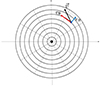 |
Fig. 1. Representation of the VRM: LOS velocity is decomposed in the polar coordinates in the plane a galaxy into a radial and transversal component. The projected image of a galaxy is divided into Nr radial shells and Na arcs. In the example Nr = 8 and Na = 12. |
To present a simple example of the coarse-grained maps of the transversal vθ and radial velocity components, we show the results for a toy disk model in Fig. 2. In this model, vθ linearly increases from 200 km/s at the center to 250 km/s at the outermost shells, while vR is zero up to half of the disk radius and then increases linearly to 66 km/s. In this case, the velocity field is isotropic, so that the VRM-reconstructed coarse-grained velocity component maps exhibit no angular anisotropy, only a radial variation. We refer to Sylos Labini et al. (2023b) for a more detailed discussion of the VRM methods and its results for toy disk models and real galactic images.
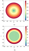 |
Fig. 2. VRM-reconstructed coarse-grained map of the transversal vθ (panel a) and radial velocity component (panel b) for a simple toy disk model with an isotropic velocity distribution (see text for more details). |
The VRM maps can be further refined by splitting each ring into Na arcs, each characterized by a different radial and transversal velocity, and it is possible to characterize velocity anisotropies, that is, the dependence of the two velocity components on the radial distance R and the angular coordinate θ, meaning that vθ = vθ(R, θ), vR = vR(R, θ). The VRM divides the galaxy image into a grid of Ncells cells that is determined by the product of the number of rings and the number of arcs, that is, Ncells = Nr × Na. Within the ith cell, the VRM provides the transverse velocity component, vθi, and the radial velocity component, vRi. It is then possible to analyze the convergence of the VRM method by studying the convergence of several moments that measure the velocity field in a given region by varying the resolution of the coarse-grained map (see Sylos Labini et al. 2023b for details).
On one hand, the size of each of the Ncells must be larger than the beam size σ, and on the other hand, enough cells are required for a reliable statistical analysis of the anisotropy structures in the coarse-grained velocity component 2D maps. The first requirement is satisfied as long as the cell size exceeds the beam size of 25″ × 25″, to which the original map is smoothed. Conversely, the optimal number of cells can be determined by analyzing the convergence of various moments (see Sylos Labini et al. 2023b for details) that characterize the velocity field within a given region as the resolution of the coarse-grained map is varied. This process involves, for instance, changing the number of arcs while keeping the number of rings fixed. The convergence of these moments that ensure that the reconstructed velocity field remains stable and independent of the resolution employed by the VRM is critical for evaluating the reliability of the method. It demonstrates that the noise introduced by the VRM reconstruction, which is inevitably present, does not dominate the signal. We report results for Nr = 10 and Na = 8 below. This corresponds to the galaxy with the lowest resolution for which cells are on the order of or larger than the beam size.
In principle, the degeneracy between warps and radial flows in external galaxies prevents us from diskriminating radial flows from geometric deformations. However, the possible warped geometry of a disk galaxy is typically more pronounced in the outermost regions, which may be affected by tidal forces from external perturbers. Some edge-on disk galaxies show warps that start at the optical radius (Sancisi 1976; Reshetnikov & Combes 1998; Schwarzkopf & Dettmar 2001; García-Ruiz et al. 2002; Sánchez-Saavedra et al. 2003). To control that the key assumption of the VRM that the disk is flat is a good working hypothesis, we therefore monitored the behavior of the orientation angles determined by the TRM as a function of the radial distance. Only when they presented a smooth radial change did we interpret the behaviors as indicating the presence of a warp. Fluctuations in the values of the orientation angles throughout the disk were interpreted as being due to velocity anisotropies in the VRM framework. In practice, when the orientation angles smoothly vary with scale, we used the circular velocity, averaged over rings, determined by the TRM. We found, however, that in general, the correction due to the warp for the galaxies in this sample is small in the inner regions of the disks, and thus vθ(R) is generally very similar to the circular velocity determined by the TRM. In a forthcoming paper (Sylos Labini et al. 2024), we will present a method for correcting the VRM determinations when the disk is warped.
3.2. Correction for asymmetric drift
Under the assumption that the galaxy is in stationary state and collisions can be neglected, we used the Jeans equations to relate the observed kinematic properties to the gravitational field of the system (Binney & Tremaine 2008). In particular, for an axisymmetric system in cylindrical R, z, θ coordinates, we have that
where ρ is mass density in the disk, vR, vθ, and vz are the radial, tangential, and vertical components of the velocity in cylindrical coordinates, respectively,  ,
,  , and
, and  are the moments of the velocity distribution, and Φ is the gravitational potential of the entire system. We refer to the mean values and fluctuations (i.e., anisotropies) of the radial and tangential velocity components throughout while disregarding variations in the vertical velocity component because it is not observable in external galaxies.
By defining the circular velocity as

we can rewrite Eq. (2) as
We neglect hereafter the terms with  as they are generally considered subdominant. While for the case of the Milky Way it is now possible to directly measure these terms and to measure that they are indeed negligible (Eilers et al. 2019; Wang et al. 2023; Ou et al. 2024), this is a reasonable working hypothesis for the case of external galaxies. Neglecting these mixed terms, we find
From the very definition of dispersion we can write that

and
We assumed  . While we lack direct observations of the vertical component, we can measure the radial component by means of the VRM method and limit the analysis to the range within which it fluctuates around zero.
Considering Eq. (6), we can rewrite Eq. (5) as
By assuming σvθ2 ≈ σvR2 ≈ σ2, where σ2 is given by second moment of the observed velocity field (moment 2), Eq. (8) becomes
where we defined the asymmetric drift as
In Eqs. (9) and (10) the kinematic terms can be measured from the data, but the density ρ(R) depends on the adopted mass model adopted. We discuss this in the next section.
The density ρ in Eq. (2) and thus in Eq. (10) corresponds to the density within the disk. In the NFW case, ρ therefore refers exclusively to the baryonic component (i.e., the stellar and gaseous components), which is dominated by the gas mass. Conversely, in the DMD model, where DM is also assumed to reside in the disk, ρ represents the combined mass density of the baryonic and DM components. For a more detailed discussion of this point, we refer to Sylos Labini (2024).
4. Mass models
The dynamics of the sample galaxies is determined by the combination of two components: the baryonic matter, and the DM. Oh et al. (2015) focused on the consideration of the halo model proposed by Navarro et al. (1996) (NFW) and the spherical pseudo-isothermal halo model introduced by Begeman et al. (1991). The NFW halo model represents a cusp-like halo, whereas the pseudo-isothermal halo exhibits a core-like behavior. In both cases, the rotation-supported disk of the galaxy is surrounded by a spherical halo consisting of DM. The difference lies in the density behavior of the halo for small radii: The NFW model follows a density profile of ρ(r)∼r−1, while the pseudo-isothermal halo maintains a constant density, ρ(r) ∼ const. We fit the NFW halo model and compare this with those obtained by Oh et al. (2015). In this model, the circular velocity can be written as (Navarro et al. 1996)
where vg(R) and vs(R) are the circular velocity due to the gas and stellar components, and vh(R) is the circular velocity of the spherical halo that is determined by the two free parameters of the model, that is, rs and ρ0, which define the NFW density profile,
where r is the 3D radius.
The circular velocity of the ith mass component in Eq. (11) is defined as the equilibrium rotational velocity that this component would induce on a test particle in the plane of the galaxy assuming it were isolated and unaffected by external influences. These velocities in the plane are calculated based on the observed stellar mass density distributions and the assumed DM distribution. While the circular velocity of the halo, vh(R), can be computed analytically, the circular velocities of the disk components, vg (gas) and vs (stars), must be determined through simulations. As the analytical calculation of the centrifugal force for a disk is not straightforward, we adopted a numerical strategy: We generated a numerical realization of a thin-disk model with the observed surface brightness of the stellar (or gas) component and the same mass. We then numerically computed the resulting centripetal acceleration (the derivation of the masses of the gaseous and stellar components was discussed in Sect. 2).
The total mass of the baryonic disk plus the halo is

where the baryonic mass Mbar is the sum of the stellar and gas components, that is,
and M200 is the mass of the halo in a sphere of radius r200, defined as the virial radius. Because the mass of the halo grows linearly at large distances, it is necessary to consider a cutoff that corresponds to the virial radius r200 where density fluctuations due to the halo are 200 times larger than the average mass density of the Universe (Navarro et al. 1996). The virial radius r200 depends on rs and ρ0.
The second model we considered was the DMD model, which assumes that DM is confined to the galaxy disk. The basis for this model can be traced back to the observed correlation between DM and the distribution of neutral hydrogen gas. This scenario assumes that the distribution of H I gas serves as a proxy for the DM distribution, which allows us to express the circular velocity as
where γs, γg are the two free parameters of the fit. They indicate how much DM is associated with the stellar and gas component. In Eq. (15) the velocity vs represents the rotation velocity induced by the stellar component on a test particle in the galaxy plane, assuming it is in isolation without external influences. Similarly, vg represents the rotation velocity induced by the gas component on the same test particle under the same conditions. These are computed by (i) estimating the surface density profiles of the stellar and gas components (the former is reported in Oh et al. 2015), (ii) generating artificial disks with these profiles, (iii) computing the gravitational potential, and (iv) making its radial derivative on the plane (i.e., Eq. (3)).
In this case, the total mass of the baryonic and dark component is
The surface density profiles of the gas and stellar components decay approximately exponentially. In this case, there is no need to consider a cutoff in distance to estimate the total mass.
The density of the disk ρ(R) that enters the Jeans equation (Eq. (2)) and thus the expression of the circular velocity (Eq. (9)) and Eq. (10) is the baryonic density for the case of the NFW model, which up to a prefactor that is not relevant in Eq. (2) is

where Σs(R) and Σg(R) are the stellar and H I; surface density, respectively. The first was measured by Oh et al. (2015), and the second was measured directly from the data of the H I (mom0). In particular, the gas surface density was computed by assuming a constant inclination angle throughout the entire disk. To remain consistent with the mass determination discussed in Sect. 2, the gas surface density was scaled up by a factor of 1.4 to account for helium and metals, while the contribution of molecular hydrogen was neglected.
The (quasi-) spherical halo was assumed be in equilibrium with a (quasi-) isotropic velocity dispersion.
For the DMD model, the density of the disk entering the Jeans equation (Eq. (2)) is given (again, up to an irrelevant prefactor) by

Specifically, it is a linear combination of the stellar and gas surface densities, rescaled by the two free parameters of the DMD model, γs and γg. This ensures that Eq. (18) remains consistent with the mass model described in Eq. (15).
In the analysis of the individual galaxies in our sample, we fit Σdmd(R) with the function
which corresponds to a cored profile. In general, we found for the galaxies in our sample that β is in the range [1, 4]. We performed a polynomial fit to σ, and we then inserted the results of the two fits in Eqs. (9) and (10) to obtain the asymmetric drift and the circular velocity vc.
We stress that from a physical perspective, the distinction between the NFW and DMD models lies in the distribution and dynamical nature of DM. In the NFW model, DM is assumed to be distributed in a (quasi-) spherical halo surrounding the galaxy. The DM in this model is supported by a (quasi-) isotropic velocity dispersion, meaning that the random motions of DM particles play a significant role in supporting the gravitational potential. On the other hand, the DMD model posits that DM is primarily confined to the galactic disk and follows the distribution of neutral hydrogen. In this model, the DM is supported by rotation, similar to the visible matter in the disk. This fundamental difference in the dynamical nature of DM between the NFW and DMD models arises from distinct evolutionary paths. The NFW model assumes a hierarchical structure formation scenario, where DM halos form through gravitational collapse and the subsequent merging of smaller structures. The DMD model, as discussed in Sylos Labini et al. (2020) and related references, proposes an alternative scenario in which galaxy formation proceeds through a top-down collapse, leading to its confinement within the disk.
5. Kinematical analysis
In this section, we present the results of the analysis obtained for one specific galaxy in our sample (CVnIdwA) to show the rotation curves and other significant findings. For a comprehensive overview of the results obtained for all other galaxies in our sample, including rotation curves and additional analyses, we refer to Appendix C, where detailed information is provided.
We first determined the H I, stellar surface, and total DMD density profiles shown in panel a of Fig. 3. The H I surface density profile was derived based on the analysis of the intensity (mom0) map. The sky-plane coordinates (r, ϕ) provided by observations were transformed into galaxy-plane coordinates (R, θ) assuming a constant inclination angle throughout the disk,
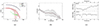 |
Fig. 3. Profiles of CVnIdwA. (a) Total DMD, H I, and stellar surface density profiles. The parameters Rg, β of the function in Eq. (19) (blue line) are reported in the panels. (b) Velocity dispersion profile σ(R) averaged in rings with a sixth-degree polynomial fit (red line). (c) Orientation angles from the TRM as a function of the radial distance: position angle (upper panel) and inclination angle (bottom panel). |
where i is the inclination angle, and ϕ0 is the PA (see Sylos Labini et al. 2023b for more details). The H I density profile was computed in concentric circular rings with a radius R and a thickness ΔR.
The stellar surface density profile was the profile measured by Oh et al. (2015) and thus has a different sampling, that is, ΔR, than that of H I. Thus, to numerically compute their sum in Eq. (17), we approximated the stellar profile by an analytical fitting function. Finally, the DMD surface brightness profile was computed from Eq. (18) after the fit with the DMD mass model was performed and the two free parameters γs and γg were determined (see Sect. 6). Panel a of Fig. 3 also shows the best of the DMD profile fit with Eq. (19) (solid line). In this case, we find that the exponent is β ≈ 1.9, which is a typical result for the galaxies in this sample.
The velocity dispersion σ was directly estimated from the moment-2 maps using a single value for the inclination angle as for the estimation of the H I surface density profile (see panel b of Fig. 3, where the behavior of the velocity dispersion, σ(R), is shown along with the sixth-degree polynomial best-fit function). We note that the values estimated for the galaxies in our sample, typically ≤15 km s−1, are consistent with those found in other dwarfs (Oh et al. 2015; Iorio et al. 2017; Di Teodoro & Peek 2021; Mancera Piña et al. 2021). The velocity dispersion for CVnIdwA decays slowly up to Rd ≈ 200″ (=1.7 kpc, assuming the distance to the galaxy is D = 3.6 Mpc; see Hunter et al. 2012) and faster beyond this radius.
The TRM analysis performed by Oh et al. (2015) provides two orientation angles: the PA (upper part of panel c of Fig. 3), and the inclination angle (bottom part of panel c of Fig. 3). The PA exhibits an approximately constant behavior for R < Rd. Beyond this radius, it clearly increases, with a change of about 20°. On the other hand, the inclination angle remains approximately constant, but shows noticeable fluctuations. The radial trend of the PA indicates a warp in the outer regions of the galaxy, while the noisy behavior of the inclination angle suggests velocity gradients.
As mentioned above, the advantage of using the VRM lies in its ability to reliably estimate the spatial anisotropies of the velocity components. The results of the VRM analysis are shown in Fig. 4. The transversal velocity (panel a of Fig. 4) presents small spatial anisotropies in the inner disk, R < Rd ≈ 150″, while larger ones are seen in the outer regions. The signal there may be affected by a warp, however. A similar situation occurs for the radial velocity map (panel b of Fig. 4). We used a resolution of ten rings and eight arcs so that the total number of cells is Ncells = 80, and each cell has a size of approximately ∼700 arcsec2, compared to the beam size of ∼625 arcsec2. We verified that the anisotropy maps converged when the number of cells changed. This is illustrated in Fig. 5, which shows the maps of the transverse and radial velocity components for different numbers of arcs Na = 2, 4, 8 and same number of rings Nr = 10. By visually inspecting the maps, it can be seen that the anisotropy structures remain approximately consistent for Na = 2, 4, 8 while the signal becomes noticeably noisier for Na = 16, 32 (not shown).
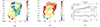 |
Fig. 4. VRM maps of CVnIdwA: (a) Transversal velocity component map with a resolution of Nr = 10 and Na = 8 and (b) radial velocity component map with a resolution of Nr = 10 and Na = 8. (c) Upper panel: Transversal velocity profile as measured by the VRM without corrections (black dots) and as determined by the TRM (red dots). Bottom panel: Radial velocity profile. |
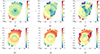 |
Fig. 5. VRM maps of CVnIdwA with varying resolution: (a, b, and c) Transversal velocity component map with a resolution of Nr = 10 and Na = 2, 4, 8. (d, e, and f) Radial velocity component map with a resolution of Nr = 10 and Na = 2, 4, 8. |
The transversal velocity profile averaged over rings is close to the circular velocity vc(R) measured by the TRM by Oh et al. (2015) (upper part of panel c of Fig. 4). The difference at large radial distances can be attributed to the effect of the warp, which is not taken into account by the VRM. The radial profile (bottom part of panel c of Fig. 4) shows large fluctuations (compared to vt(R)) beyond ≈Rd. From these behaviors, we conclude that for R < Rd, the disk is in rotational equilibrium. Beyond Rd, perturbations from a steady state can be relevant.
As mentioned above, the best VRM was determined by minimizing the residuals, that is, the differences between the observed and modeled velocities, with respect to the free parameters of the model in Eq. (1). The number of free parameters is given by Npar = 2NaNr = 2Ncells, where Ncells represents the number of cells, each with two free parameters: the radial and tangential velocity components (see Sylos Labini et al. 2023b for more details). For CVnIdwA3, the residuals are small. In the inner disk, they are < 2 km/s, and in the outer disk, they are < 4 km/s (see Fig. 6). This corresponds to ∼10% and ∼20% of the peak velocity. This residual map is representative of all other galaxies, whose residual maps are not shown.
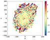 |
Fig. 6. Residual field map of CVnIdwA with a resolution of Nr = 10 and Na = 8. |
6. Mass estimation
In this section, we provide the fitting results using the DMD and NFW models for all the galaxies in our sample.
We determined the tangential velocity, vθ(R), averaged in rings and measured through the VRM, to estimate the circular velocity, which was then used to perform fits with theoretical mass models. As mentioned above, we generally found that vθ(R) agrees well within the range of distances of interest (i.e., in the inner disk) with the circular velocity determined by the TRM. Differences are typically observed at larger radii, but these are expected due to the different assumptions.
The second quantity required to compute the circular velocity (see Eq. (9)) is the asymmetric drift correction, σD2, which was estimated as explained in Sect. 3.2. This correction is close to the one determined by Oh et al. (2015), but some differences can be detected due to the different methods used to determine it.
In summary, vθ(R) and σD2 were measured differently from the corresponding quantities in Oh et al. (2015). Nevertheless, given the limited range of scales over which the fits were performed, our estimates of vc(R) and theirs agree well in most cases. This is also the case for the comparison with the results of Iorio et al. (2017) and Mancera Piña et al. (2022). In particular, the latter authors reported that H I flaring can impact the shape of the rotation curve in the outer regions of galaxies and can consequently alter the values of the best-fit parameters of the considered mass models for some LITTLE THINGS dwarfs, such as CVnIdwA. However, we note that these changes are limited in amplitude, and although consistent with the error bars of the VRM results, they primarily impact the outermost regions of galaxies, where differences due to the methods used to recover the velocity from the LOS maps, that is, VRM or TRM, become more significant. As discussed above, radial motions are typically detected by the VRM precisely in these external regions.
In some cases, we limited the fit to a smaller radius than was considered by Oh et al. (2015) because the VRM indicates that in the outer parts of the disks, the velocity field is generally more perturbed. For this reason, we focused on the range of distances in which the tangential velocity component is larger than the radial component. Additionally, the radial range over which the fits were performed typically spans less than half a decade, and in many cases, only one-third of a decade (e.g., for CVnIdwA3, the best fit with the mass models was obtained in the range 0−2.0 kpc, i.e., R < Rd). As a result, even small differences in the data points of vc can lead to significant variations in the derived model parameters. From a quantitative perspective, differences therefore exist in some cases in the estimated parameters of the NFW model (those that can be compared), and consequently, in the virial mass, M200.
The best-fit parameters for the two models were obtained by minimizing the χ2 value between the circular and observed model velocity. The errors on the two parameters of each model, γs and γg for the DMD model and Rs and ρ0 for the NFW model, were derived from the diagonal elements of the covariance matrix. From these errors, we can easily compute the errors on the total mass, Mdmd and M200, using error propagation. The results for all galaxies are reported in Table A.1. The fits of individual galaxies are shown in Fig. 7 and also in Figs. B.1 and B.2.
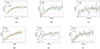 |
Fig. 7. Best fit with the DMD and NFW models for some of the galaxies in our sample: CVnIdwA (a), DDO43 (b), DDO46 (c), DDO47 (d), DDO50 (e), and DDO52 (f). The circular velocity due to the stellar and gas components is also shown. For comparison, we report in some cases the asymmetric drift-corrected rotation curves measured by Iorio et al. (2017, Iorio+17) and Mancera Piña et al. (2022, MP+22). For the other fits of the rotation curves, see Figs. B.1 and B.2. |
It is interesting to compare the results of the DMD mass model for disk and dwarf galaxies. Figure 8 illustrates the parameter space γs − γg for the disk galaxies in the THINGS sample (from Sylos Labini et al. 2024) and the dwarf galaxies in the LITTLE THINGS sample. The galaxies in the LITTLE THINGS sample generally have higher values of γs, which implies that the DM associated with the stellar component is more significant than the THINGS sample. As a result, the DM associated with the stellar component becomes much more important for the dynamics of these disk galaxies than the dwarf galaxies in the THINGS sample.
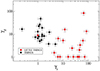 |
Fig. 8. Parameter space γs − γg for the THINGS galaxies and the LITTLE THINGS sample. |
7. Conclusions
The velocity fields of the 22 late-type dwarf galaxies in the subsample of the LITTLE THINGS survey (Hunter et al. 2012) that we considered show highly perturbed characteristics. This is evident from the simple visual inspection of the observed 2D map of the line-of-sight velocity, vlos. In almost all cases, the kinematic axis of the galaxy, that is, the axis along which vlos has the highest velocity gradient, changes orientation with radius, so that the velocity map is not symmetrical with respect to the major axis of the projected galaxy image, as would be expected for a flat, rotating disk. These irregularities in the observed velocity field are usually interpreted as resulting from local deformations of the disk, which is warped instead of being flat. While this is certainly a possible explanation for the observed maps, it may neglect the effects of noncircular motions. Warps are typically observed in the outermost regions of disk galaxies, but tend to be absent in the inner regions. Given the relatively small spatial extent of the dwarf galaxies in the subsample considered, it is thus possible that noncircular motions, rather than warps, are the primary source of the radial change in the orientation of the kinematic axis of the galaxy.
We therefore analyzed these galaxies using the velocity ring model (Sylos Labini et al. 2023b). Under the assumption of a flat disk, this allows for the reconstruction not only of the radial behaviors, averaged in rings, of the transversal and radial velocity components, but also their coarse-grained spatial maps that can trace the distribution of anisotropies. While the tilted ring model finds that some of the galaxies exhibit clear warping, thereby invalidating the assumption of a flat disk to describe their geometry, many lack the typical signature of a warp that manifests as a smooth radial dependence of the orientation angles on the radial distance in the outermost regions of the galaxy. They instead show orientation angles that are characterized by significant fluctuations. In the VRM framework, this correspond to velocity anisotropies. Consequently, through examining the inner parts of the disk, we infer that velocity anisotropies are generally significant and indicate the perturbed nature of the velocity fields in this sample of dwarf galaxies.
We then performed the best fit using two different mass models to the transversal velocity of these galaxies in the inner regions of the disk, where the assumption that they are supported by rotation appears to be well satisfied and where the geometric deformations due to a possible warp are generally negligible.
The dark matter disk (DMD) model assumes consistently with the Bosma effect (Bosma 1981) that the distribution of DM is confined to the disk and follows the same exponential decay as the gas. In the DMD model, two free parameters, γs and γg, are introduced that correspond to how much DM is associated with the stellar and gas component, respectively. This model was shown to describe the velocity field of the Milky Way (Sylos Labini et al. 2023a) and of the disk disk galaxies from the THINGS sample well (Sylos Labini et al. 2024).
The results of the DMD fits for the 22 dwarf galaxies in the su-sample of the LITTLE THINGS survey that exhibit rotation-dominated inner regions (Oh et al. 2015) are presented in Table A.1. It is worth noting that the total mass of the disk is 40 times that of the baryonic components at most. Table A.1 also includes the virial mass obtained by fitting the same rotation curves with a standard Navarro-Frenk-White (NFW) halo model (Navarro et al. 1996). The virial mass is hundreds to thousands of times higher than the baryonic mass and much higher than the total mass in the DMD model. This result is expected since in the DMD model, the DM is confined to the disk and not spread out in a large spherical region around the baryonic disk. The potential of a disk is stronger than that of a halo. With less mass, it can therefore provide the same contribution to the circular speed (Binney & Tremaine 2008; Mancera Piña et al. 2022). Additionally, in the DMD model, the radius of the disk is determined by that of the neutral hydrogen (H I) distribution, which is much smaller than the virial radius in the NFW model (i.e., the scale at which the density of the system is 200 times the average density of the Universe). This difference means that the total mass in the DMD model is much lower than that required by the NFW model (see Fig. 9).
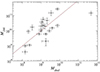 |
Fig. 9. Virial mass estimated from the NFW mass model fit vs. the disk mass obtained from the DMD model fit. The reference line corresponds to M200 = 10 × Mdmd. |
One of the notable outcomes of the DMD model is its ability to naturally address the core/cusp problem. The standard DM halo profile predicts a density distribution that follows ρ(r)∼r−1 as r approaches zero, leading to a cuspy central density profile. However, numerous observations indicated that the rotational velocity profiles of galaxies correspond to a flat density profile in the central regions. In the DMD model, the mass density profile can be computed as the weighted sum of the stellar and H I surface density profiles, where the weights are the two parameters of the DMD fit, that is, γs and γg. In general, the two profiles are flat at small radii, and so is the total mass density profile, that is, ρ(R)∼ ∝ r−α ∼ const., with α = 0. In this situation, it is expected that the rotational velocity increases linearly as a function of the radius vc ∝ r(2 − α)/2 ∼ r. This agrees with the findings of Oh et al. (2015) and supports the notion that the DMD model can reproduce the observed linear rotational velocity profiles in the central regions of galaxies. Thus, the DMD model provides a consistent explanation for the observed behavior of the rotational velocities, which is in contrast to the cuspy density profiles predicted by the standard NFW halo model.
The scales over which dwarf galaxy disks extend, typically not more than 5 kpc, are not directly relevant to cosmology. Therefore, the estimate of the DM content for these objects does not have a direct impact on cosmological parameters. The key question posed by the DMD model is the quantification of the degree of flatness in the distribution of DM. In particular, it seeks to determine whether the DM distribution resembles a closer-to-spherical system or a flatter axially symmetric disk. This question cannot be directly answered by analyzing the projected images of galaxies, as this analysis only reveals the degree of compatibility between observed velocity and density fields and a given model. Instead, there are two types of observations that can probe the degree of flatness in the overall mass distribution of certain disk galaxies in principle. First, the study of off-plane motions in our own Galaxy or neighboring galaxies can provide insights. Second, the analysis of high-precision gravitational-lensing measurements of distant objects by nearby disk galaxies represents a powerful means to investigate the shape of a galaxy mass distribution. Forthcoming works will be devoted to the study of these issues.
Data availability
Appendix C is available at this url https://doi.org/10.5281/zenodo.14438509
Spitzer Space Telescope https://science.nasa.gov/mission/spitzer/
Acknowledgments
We thank Michael Joyce for valuable discussions. We also acknowledge an anonymous referee for their detailed comments and suggestions, which have significantly improved our presentation.
References
- Barnes, E. I., & Sellwood, J. A. 2003, AJ, 125, 1164 [NASA ADS] [CrossRef] [Google Scholar]
- Begeman, K. G., Broeils, A. H., & Sanders, R. H. 1991, MNRAS, 249, 523 [Google Scholar]
- Benhaiem, D., Sylos Labini, F., & Joyce, M. 2019, Phys. Rev. E, 99, 022125 [Google Scholar]
- Binney, J., & Tremaine, S. 2008, Galactic Dynamics (Princeton: Princeton University Press) [Google Scholar]
- Bosma, A. 1978, Ph.D. Thesis, University of Groningen, The Netherlands [Google Scholar]
- Bosma, A. 1981, AJ, 86, 1791 [NASA ADS] [CrossRef] [Google Scholar]
- Casandjian, J.-M., Ballet, J., Grenier, I., & Remy, Q. 2022, ApJ, 940, 116 [NASA ADS] [CrossRef] [Google Scholar]
- Combes, F., & Pfenniger, D. 1997, A&A, 327, 453 [NASA ADS] [Google Scholar]
- Dabringhausen, J., & Kroupa, P. 2013, MNRAS, 429, 1858 [NASA ADS] [CrossRef] [Google Scholar]
- de Blok, W. J. G., & Bosma, A. 2002, A&A, 385, 816 [CrossRef] [EDP Sciences] [Google Scholar]
- de Blok, W. J. G., McGaugh, S. S., & van der Hulst, J. M. 1996, MNRAS, 283, 18 [NASA ADS] [CrossRef] [Google Scholar]
- de Blok, W. J. G., McGaugh, S. S., & Rubin, V. C. 2001, AJ, 122, 2396 [NASA ADS] [CrossRef] [Google Scholar]
- Diemand, J., Kuhlen, M., Madau, P., et al. 2008, Nature, 454, 735 [NASA ADS] [CrossRef] [Google Scholar]
- Di Teodoro, E. M., & Fraternali, F. 2015, MNRAS, 451, 3021 [Google Scholar]
- Di Teodoro, E. M., & Peek, J. E. G. 2021, ApJ, 923, 220 [NASA ADS] [CrossRef] [Google Scholar]
- Eilers, A.-C., Hogg, D. W., Rix, H.-W., & Ness, M. K. 2019, ApJ, 871, 120 [Google Scholar]
- Einasto, J. 1965, Trudy Astrofizicheskogo Instituta Alma-Ata, 5, 87 [NASA ADS] [Google Scholar]
- Fraternali, F., Oosterloo, T., Sancisi, R., & van Moorsel, G. 2001, ApJ, 562, L47 [CrossRef] [Google Scholar]
- García-Ruiz, I., Sancisi, R., & Kuijken, K. 2002, A&A, 394, 769 [NASA ADS] [CrossRef] [EDP Sciences] [Google Scholar]
- Grenier, I. A., Casandjian, J.-M., & Terrier, R. 2005, Science, 307, 1292 [Google Scholar]
- Hessman, F. V., & Ziebart, M. 2011, A&A, 532, A121 [NASA ADS] [CrossRef] [EDP Sciences] [Google Scholar]
- Hoekstra, H., van Albada, T. S., & Sancisi, R. 2001, MNRAS, 323, 453 [NASA ADS] [CrossRef] [Google Scholar]
- Hunter, D. A., & Elmegreen, B. G. 2006, ApJS, 162, 49 [NASA ADS] [CrossRef] [Google Scholar]
- Hunter, D. A., Ficut-Vicas, D., Ashley, T., et al. 2012, AJ, 144, 134 [CrossRef] [Google Scholar]
- Iorio, G., Fraternali, F., Nipoti, C., et al. 2017, MNRAS, 466, 4159 [NASA ADS] [Google Scholar]
- Ishiyama, T., Rieder, S., Makino, J., et al. 2013, ApJ, 767, 146 [NASA ADS] [CrossRef] [Google Scholar]
- Kennicutt, R. C., Armus, L., Bendo, G., et al. 2003, PASP, 115, 928 [NASA ADS] [CrossRef] [Google Scholar]
- Kroupa, P. 2012, PASA, 29, 395 [NASA ADS] [CrossRef] [Google Scholar]
- Lazar, A., Bullock, J. S., Boylan-Kolchin, M., et al. 2020, MNRAS, 497, 2393 [NASA ADS] [CrossRef] [Google Scholar]
- Mancera Piña, P. E., Posti, L., Fraternali, F., Adams, E. A. K., & Oosterloo, T. 2021, A&A, 647, A76 [NASA ADS] [CrossRef] [EDP Sciences] [Google Scholar]
- Mancera Piña, P. E., Fraternali, F., Oosterloo, T., et al. 2022, MNRAS, 514, 3329 [CrossRef] [Google Scholar]
- Moore, B. 1994, Nature, 370, 629 [NASA ADS] [CrossRef] [Google Scholar]
- Moore, B., Ghigna, S., Governato, F., et al. 1999, ApJ, 524, L19 [Google Scholar]
- Navarro, J. F., Eke, V. R., & Frenk, C. S. 1996, MNRAS, 283, L72 [NASA ADS] [Google Scholar]
- Navarro, J. F., Frenk, C. S., & White, S. D. M. 1997, ApJ, 490, 493 [Google Scholar]
- Navarro, J. F., Hayashi, E., Power, C., et al. 2004, MNRAS, 349, 1039 [Google Scholar]
- Navarro, J. F., Ludlow, A., Springel, V., et al. 2010, MNRAS, 402, 21 [Google Scholar]
- Oh, S.-H., de Blok, W. J. G., Walter, F., Brinks, E., & Kennicutt, R. C. 2008, AJ, 136, 2761 [NASA ADS] [CrossRef] [Google Scholar]
- Oh, S.-H., de Blok, W. J. G., Brinks, E., Walter, F., & Kennicutt, R. C. 2011, AJ, 141, 193 [NASA ADS] [CrossRef] [Google Scholar]
- Oh, S.-H., Hunter, D. A., Brinks, E., et al. 2015, AJ, 149, 180 [CrossRef] [Google Scholar]
- Ou, X., Eilers, A.-C., Necib, L., & Frebel, A. 2024, MNRAS, 528, 693 [NASA ADS] [CrossRef] [Google Scholar]
- Pawlowski, M. S., & Kroupa, P. 2013, MNRAS, 435, 2116 [NASA ADS] [CrossRef] [Google Scholar]
- Pfenniger, D., Combes, F., & Martinet, L. 1994, A&A, 285, 79 [NASA ADS] [Google Scholar]
- Planck Collaboration XIX. 2011, A&A, 536, A19 [NASA ADS] [CrossRef] [EDP Sciences] [Google Scholar]
- Power, C., Navarro, J. F., Jenkins, A., et al. 2003, MNRAS, 338, 14 [Google Scholar]
- Read, J. I., Iorio, G., Agertz, O., & Fraternali, F. 2016, MNRAS, 462, 3628 [NASA ADS] [CrossRef] [Google Scholar]
- Reshetnikov, V., & Combes, F. 1998, A&A, 337, 9 [NASA ADS] [Google Scholar]
- Retana-Montenegro, E., van Hese, E., Gentile, G., Baes, M., & Frutos-Alfaro, F. 2012, A&A, 540, A70 [NASA ADS] [CrossRef] [EDP Sciences] [Google Scholar]
- Rogstad, D. H., Lockhart, I. A., & Wright, M. C. H. 1974, ApJ, 193, 309 [Google Scholar]
- Sánchez-Saavedra, M. L., Battaner, E., Guijarro, A., López-Corredoira, M., & Castro-Rodríguez, N. 2003, A&A, 399, 457 [NASA ADS] [CrossRef] [EDP Sciences] [Google Scholar]
- Sancisi, R. 1976, A&A, 53, 159 [NASA ADS] [Google Scholar]
- Sancisi, R. 1999, Astrophys. Space Sci., 269, 59 [NASA ADS] [CrossRef] [Google Scholar]
- Schmidt, T. M., Bigiel, F., Klessen, R. S., & de Blok, W. J. G. 2016, MNRAS, 457, 2642 [NASA ADS] [CrossRef] [Google Scholar]
- Schwarzkopf, U., & Dettmar, R.-J. 2001, A&A, 373, 402 [NASA ADS] [CrossRef] [EDP Sciences] [Google Scholar]
- Sellwood, J. A., & Sánchez, R. Z. 2010, MNRAS, 404, 1733 [NASA ADS] [Google Scholar]
- Sellwood, J. A., Spekkens, K., & Eckel, C. S. 2021, MNRAS, 502, 3843 [NASA ADS] [CrossRef] [Google Scholar]
- Spekkens, K., & Sellwood, J. A. 2007, ApJ, 664, 204 [NASA ADS] [CrossRef] [Google Scholar]
- Stadel, J., Potter, D., Moore, B., et al. 2009, MNRAS, 398, L21 [NASA ADS] [CrossRef] [Google Scholar]
- Swaters, R. A., Sancisi, R., van der Hulst, J. M., & van Albada, T. S. 2012, MNRAS, 425, 2299 [NASA ADS] [CrossRef] [Google Scholar]
- Sylos Labini, F. 2024, ApJ, 976, 185 [CrossRef] [Google Scholar]
- Sylos Labini, F., Pinto, L. D., & Capuzzo-Dolcetta, R. 2020, Phys. Rev. E, 102, 042108 [Google Scholar]
- Sylos Labini, F., Chrobáková, Ž., Capuzzo-Dolcetta, R., & López-Corredoira, M. 2023a, ApJ, 945, 3 [NASA ADS] [CrossRef] [Google Scholar]
- Sylos Labini, F., Straccamore, M., De Marzo, G., & Comerón, S. 2023b, MNRAS, 524, 1560 [Google Scholar]
- Sylos Labini, F., De Marzo, G., Straccamore, M., & Comerón, S. 2024, MNRAS, 527, 2697 [Google Scholar]
- Walter, F., Cannon, J. M., Roussel, H., et al. 2007, ApJ, 661, 102 [NASA ADS] [CrossRef] [Google Scholar]
- Walter, F., Brinks, E., de Blok, W. J. G., et al. 2008, AJ, 136, 2563 [Google Scholar]
- Wang, E., & Lilly, S. J. 2023, ApJ, 944, 143 [NASA ADS] [CrossRef] [Google Scholar]
- Wang, H.-F., Chrobáková, Ž., López-Corredoira, M., & Sylos Labini, F. 2023, ApJ, 942, 12 [NASA ADS] [CrossRef] [Google Scholar]
- Warner, P. J., Wright, M. C. H., & Baldwin, J. E. 1973, MNRAS, 163, 163 [NASA ADS] [Google Scholar]
Appendix A: Table
Table A.1 shows the parameters of the mass model fits.
Results of the mass models fits
Appendix B: Fits of rotation curves
Figures B.1 and B.2 show the remaining fits of the rotation curves of the galaxies not displayed in Fig. 7.
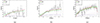 |
Fig. B.1. Best fit with the DMD and NFW models for some of the galaxies in our sample. The circular velocity due to the stellar and gas components is also shown. For comparison, in some cases, we have reported the asymmetric drift-corrected rotation curves measured by Iorio et al. (2017) (Iorio+17) and Mancera Piña et al. (2022) (MP+22). |
All Tables
All Figures
|
Fig. 1. Representation of the VRM: LOS velocity is decomposed in the polar coordinates in the plane a galaxy into a radial and transversal component. The projected image of a galaxy is divided into Nr radial shells and Na arcs. In the example Nr = 8 and Na = 12. |
| In the text | |
|
Fig. 2. VRM-reconstructed coarse-grained map of the transversal vθ (panel a) and radial velocity component (panel b) for a simple toy disk model with an isotropic velocity distribution (see text for more details). |
| In the text | |
|
Fig. 3. Profiles of CVnIdwA. (a) Total DMD, H I, and stellar surface density profiles. The parameters Rg, β of the function in Eq. (19) (blue line) are reported in the panels. (b) Velocity dispersion profile σ(R) averaged in rings with a sixth-degree polynomial fit (red line). (c) Orientation angles from the TRM as a function of the radial distance: position angle (upper panel) and inclination angle (bottom panel). |
| In the text | |
|
Fig. 4. VRM maps of CVnIdwA: (a) Transversal velocity component map with a resolution of Nr = 10 and Na = 8 and (b) radial velocity component map with a resolution of Nr = 10 and Na = 8. (c) Upper panel: Transversal velocity profile as measured by the VRM without corrections (black dots) and as determined by the TRM (red dots). Bottom panel: Radial velocity profile. |
| In the text | |
|
Fig. 5. VRM maps of CVnIdwA with varying resolution: (a, b, and c) Transversal velocity component map with a resolution of Nr = 10 and Na = 2, 4, 8. (d, e, and f) Radial velocity component map with a resolution of Nr = 10 and Na = 2, 4, 8. |
| In the text | |
|
Fig. 6. Residual field map of CVnIdwA with a resolution of Nr = 10 and Na = 8. |
| In the text | |
|
Fig. 7. Best fit with the DMD and NFW models for some of the galaxies in our sample: CVnIdwA (a), DDO43 (b), DDO46 (c), DDO47 (d), DDO50 (e), and DDO52 (f). The circular velocity due to the stellar and gas components is also shown. For comparison, we report in some cases the asymmetric drift-corrected rotation curves measured by Iorio et al. (2017, Iorio+17) and Mancera Piña et al. (2022, MP+22). For the other fits of the rotation curves, see Figs. B.1 and B.2. |
| In the text | |
|
Fig. 8. Parameter space γs − γg for the THINGS galaxies and the LITTLE THINGS sample. |
| In the text | |
|
Fig. 9. Virial mass estimated from the NFW mass model fit vs. the disk mass obtained from the DMD model fit. The reference line corresponds to M200 = 10 × Mdmd. |
| In the text | |
|
Fig. B.1. Best fit with the DMD and NFW models for some of the galaxies in our sample. The circular velocity due to the stellar and gas components is also shown. For comparison, in some cases, we have reported the asymmetric drift-corrected rotation curves measured by Iorio et al. (2017) (Iorio+17) and Mancera Piña et al. (2022) (MP+22). |
| In the text | |
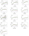 |
Fig. B.2. Same as Fig. 7 but for the remaining galaxies in the sample). |
| In the text | |
Current usage metrics show cumulative count of Article Views (full-text article views including HTML views, PDF and ePub downloads, according to the available data) and Abstracts Views on Vision4Press platform.
Data correspond to usage on the plateform after 2015. The current usage metrics is available 48-96 hours after online publication and is updated daily on week days.
Initial download of the metrics may take a while.