| Issue |
A&A
Volume 693, January 2025
|
|
|---|---|---|
| Article Number | A56 | |
| Number of page(s) | 7 | |
| Section | Astrophysical processes | |
| DOI | https://doi.org/10.1051/0004-6361/202451836 | |
| Published online | 03 January 2025 | |
The impact of resistivity on the variability of black hole accretion flows
1
Research Center for Astronomy and Applied Mathematics, Academy of Athens, Athens 11527, Greece
2
Institut für Theoretische Physik, Goethe Universität Frankfurt, Max-von-Laue-Str.1, 60438 Frankfurt am Main, Germany
3
Tsung-Dao Lee Institute, Shanghai Jiao Tong University, Shanghai 201210, China
4
School of Physics and Astronomy, Shanghai Jiao Tong University, Shanghai 200240, China
5
Institut für Theoretische Physik und Astrophysik, Universität Würzburg, Emil-Fischer-Strasse 31, 97074 Würzburg, Germany
6
Max-Planck-Institut für Radioastronomie, Auf dem Hügel 69, D-53121 Bonn, Germany
7
Instituto de Astronomía, Universidad Nacional Autónoma de México, AP 70-264, 04510 Ciudad de México, Mexico
8
Instituto de Astrofísica de Andalucía, Gta. de la Astronomía, s/n, Genil, 18008 Granada, Spain
9
School of Mathematics, Trinity College, Dublin 2, Ireland
10
Frankfurt Institute for Advanced Studies, Ruth-Moufang-Str. 1, 60438 Frankfurt am Main, Germany
⋆ Corresponding author; anathanail@academyofathens.gr
Received:
8
August
2024
Accepted:
19
November
2024
Context. The accretion of magnetized plasma onto black holes is a complex and dynamic process in which the magnetic field plays a crucial role. The amount of magnetic flux that is accumulated near the event horizon significantly impacts the accretion flow behavior. Resistivity, which is a measure of how easily magnetic fields can dissipate, is thought to be a key factor influencing this process.
Aims. This work explores the influence of resistivity on the accretion flow variability. We investigated simulations that reached the limit of the magnetically arrested disk (MAD) and simulations with an initial multi-loop magnetic field configuration.
Methods. We employed 3D resistive general relativistic magnetohydrodynamic (MHD) simulations to model the accretion process under various regimes, where resistivity is globally constant (uniform resistivity).
Results. Our findings reveal distinct flow behaviors depending on resistivity. High-resistivity simulations never achieved the MAD state, which indicates a disturbed magnetic-flux accumulation process. Conversely, low-resistivity simulations converged toward the ideal MHD limit. The key results are that i) for the standard MAD model, resistivity plays a minimum role in flow variability, suggesting that flux eruption events dominate the dynamics. ii) High-resistivity simulations exhibit strong magnetic field diffusion into the disk that rearranges the efficient magnetic flux accumulation from the accretion flow. iii) In multi-loop simulations, resistivity significantly reduces the flow variability, which was not expected. However, magnetic flux accumulation becomes more variable as a result of frequent reconnection events at very low resistivity values.
Conclusions. This study shows that resistivity affects how much the flow is distorted as a result of the magnetic field dissipation. Our findings provide new insights into the interplay between magnetic field accumulation, resistivity, variability, and the dynamics of black hole accretion.
Key words: accretion / accretion disks / black hole physics / magnetic reconnection / magnetohydrodynamics (MHD)
© The Authors 2024
 Open Access article, published by EDP Sciences, under the terms of the Creative Commons Attribution License (https://creativecommons.org/licenses/by/4.0), which permits unrestricted use, distribution, and reproduction in any medium, provided the original work is properly cited.
This article is published in open access under the Subscribe to Open model. Subscribe to A&A to support open access publication.
1. Introduction
The accretion of plasma onto black holes is the basis for studying and analyzing observations of black holes. More specifically, the supermassive black hole, Sgr A*, located at the center of our Galaxy, and M87* have served as subjects for numerous multiwavelength observation campaigns (Falcke et al. 1998; Baganoff et al. 2001; Genzel et al. 2003; Doeleman et al. 2008; Hada et al. 2013; Kim et al. 2018). The Event Horizon Telescope (EHT) Collaboration has recently achieved a remarkable milestone by capturing groundbreaking images of black holes that revealed a luminous ring surrounding a prominent black hole shadow (Event Horizon Telescope Collaboration 2019a, 2022a) and an ordered magnetic field, which favors a magnetically arrested disk (MAD) state (Event Horizon Telescope Collaboration 2021, 2024). These observations highlight the limitations of current theoretical models in explaining the variability observed in the light curves of these objects (Event Horizon Telescope Collaboration 2022b). Understanding and characterizing this variability is essential for interpreting both black hole images and light-curve data (Burke et al. 2021; Broderick et al. 2022; Georgiev et al. 2022; Satapathy et al. 2022).
The MAD models are commonly used to describe active galactic nuclei (AGN) with jets (Bisnovatyi-Kogan & Ruzmaikin 1974; Narayan et al. 2003; Cruz-Osorio et al. 2022; Fromm et al. 2022). As the accretion progresses, magnetic flux accumulates near the black hole event horizon. The resulting magnetic pressure eventually balances the ram pressure of the disk, reaching equipartition and significantly impeding further accretion (Igumenshchev et al. 2003; Igumenshchev 2008; Tchekhovskoy et al. 2011). However, three-dimensional nonaxisymmetric processes such as the magnetic Rayleigh – Taylor instability, allow for continued accretion (Papadopoulos & Contopoulos 2019).
Resistivity plays a crucial role by influencing the magnetic reconnection process itself. The angular momentum transport and the amplitude of the magnetic energy after saturation can be significantly reduced by finite resistivity, as the magnetorotational instability (MRI) can be influenced under certain conditions in the disk, which would in turn affect the angular momentum transport (Pandey & Wardle 2012). A common approach to modeling such situation, is to introduce a global constant value for resistivity in relativistic MHD simulations (Del Zanna et al. 2016; Ripperda et al. 2019a; Mattia et al. 2023). However, a more realistic and physically motivated model for resistivity is needed that considers its nonuniform nature. Ideally, resistivity should be significant only on local scales, such as in X-points where reconnection occurs, but leave the global dynamics largely unaffected (Selvi et al. 2023). A similar investigation took place in 2012 in pulsars but was soon replaced by particle-in-cell simulations (Li et al. 2012; Kalapotharakos et al. 2012).
This study investigates the impact of resistivity on the dynamics of the accretion flow using a global prescription to describe this effect. We present results of 3D general relativistic magnetohydrodynamic (GRMHD) simulations for resistive MAD models and also accretion models with an initial multi-loop magnetic field configuration, in which there is no steady magnetized funnel above the black hole, but in which reconnecting current sheets are periodically formed (Nathanail et al. 2020a,b; Chashkina et al. 2021). The latter scenario may be specifically relevant for modeling the future observations of the galactic center, Sgr A* (Nathanail et al. 2022a). It is important to note that resistivity was thought to affect the variability in the accretion process very little, let alone reduce it. However, a key and unexpected result of our study is that the inclusion of resistivity does influence and even lowers the variability for a specific accretion model, that is, for the multi-loop model.
The paper is structured as follows: In Section 2 we present our simulations. Section 2.1 focuses on the numerical setup, and Section 2.2 reports the details of the accretion process. In Section 2.3 we analyze and discuss the variability in the accretion flow, and in Section 3 we present our conclusions.
2. Resistive GRMHD simulations
2.1. Numerical setup
The numerical configuration comprised a Kerr black hole spacetime and an initially perturbed torus infused with a poloidal magnetic field. All simulations conducted in this study were performed in three spatial dimensions, employing the GRMHD code BHAC (Porth et al. 2017). This code uses second-order shock-capturing finite-volume methods and has been extensively used in various investigations (Nathanail et al. 2019, 2020b; Mizuno et al. 2018). It employs the constrained-transport method (Del Zanna et al. 2007) to ensure a divergence-free magnetic field (Olivares et al. 2019) and has undergone comprehensive testing and comparisons with similar-capability GRMHD codes (Porth et al. 2019).
We explored two sets of models: a MAD configuration and multi-loop configurations. For the first configuration, the initial data consisted of an equilibrium torus with a constant specific angular momentum of ℓ = 6.76 (Fishbone & Moncrief 1976) orbiting a Kerr black hole with dimensionless spins of a = 0.937. The magnetic field was initialized as a nested loop described by the vector potential
where the maximum rest-mass density in the torus is denoted with ρmax.
For the multi-loop models and a spin of a = 0.5 and ℓ = 4.28, the initial magnetic field consisted of a series of nested loops with alternating polarity. The vector potential has the form

and the additional parameters (N = 3 and λr = 2) set the number and characteristic length-scale of the initial magnetic loops in the torus. Similar configurations have been thoroughly presented and analyzed in 2D and 3D (Parfrey et al. 2015; Yuan et al. 2019a,b; Mahlmann et al. 2020). Two-temperature GRMHD simulations with a multi-loop magnetic field were also conducted to trace electron heating through turbulence and reconnection. The findings suggested that the electrons are often trapped in plasmoids (Jiang et al. 2023). Additionally, these simulations investigated the emission properties of the plasmoids (Jiang et al. 2024).
The computational domain adopted a spherical logarithmic Kerr-Schild coordinate system. In Table 1 we report all our 3D simulations. The initial field strength was set by the value of 2pmax/(B2)max, where the location of the maximum fluid and magnetic pressure may not coincide. The ideal MAD model, MAD.S.100.E.00, is the standard MAD model in the literature. For comparison, the same model was run with a resistivity η = 5 × 10⁻⁶, named MAD.S.100.E.−6. To study the effect of the magnetic field dissipation and its impact on the dynamics of the flow, we increased the field strength for the remaining models, which resulted in a maximum initial magnetization that was higher by a factor of 2. The effective resolution is reported in Col. 6 of Table 1. The models MAD.S.26.E.−5.HR, ML.S.26.E.00, and ML.S.26.E.−5 with the highest resolution ended at t = 5000 M.
Initial parameters for the models.
For the simulations with a physical resistivity, that is, η ≠ 0, we employed the resistive GRMHD equations implemented in BHAC (Ripperda et al. 2019a). In this setup, we assumed a globally constant resistivity with a varying value of η = 5 × 10⁻³ − 10−61. The choice of a small resistivity, η = 5 × 10⁻⁵ and η = 5 × 10⁻⁶, was deliberate because it allowed us to replicate nearly ideal conditions for the accretion flow dynamics but also permitted a physical magnetic reconnection processes that might lead to the formation of plasmoids (Ripperda et al. 2019b, 2020).
When we consider the gravitational radius, L ≈ rg, as the characteristic length scale, a resistivity of η = 5 × 10⁻⁶ in the jets of supermassive black holes yields a high Lundquist number of S = LuA/η = rgc/η > 104, the magnetization is strong, and the Alfvèn speed approaches the speed of light uA ≈ c (Guo et al. 2015). This value represents the minimum Lundquist number required to generate plasmoids under the physical conditions examined in this study (Bhattacharjee et al. 2009; Uzdensky et al. 2010; Ripperda et al. 2019b, 2020). However, we also employed values of resistivity that were higher than the minimum value to explore its impact on the properties of the accretion flow and on the induced variability.
In the ideal GRMHD models (see Table 1), the dissipation of magnetic energy is solely a numerical effect. However, previous 2D simulations demonstrated that a higher resolution still allows us to obtain physically meaningful results. These allow a more detailed study of the solution behavior (Obergaulinger et al. 2009; Rembiasz et al. 2017; Nathanail et al. 2020a; Obergaulinger & Aloy 2020).
2.2. Properties of the accretion flow
Our work primarily focuses on a single aspect: investigating the influence of resistivity on the variability in the accretion flow. To analyze the main properties of the accretion dynamics, we defined the rest-mas accretion rate and the magnetic flux across the horizon. The former is measured as:
where ρ is the rest-mas density, ur is the radial component of the four velocity, and  is the determinant of the spacetime metric. Its behavior is reported as a function of time in the upper panels of Figs. 1 and 2. The left panels refer to two MAD models, and the right panels show the multi-loop models. The magnetic flux accreted across the event horizon is defined as
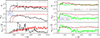 |
Fig. 1. Dynamics of the accretion flow. The two panels show the ideal and resistive case for MAD models (left panels) and Multi-loop models (right panels). Upper panels: Mass accretion rate, Ṁ, through the black hole horizon. Middle panels: Magnetic flux accumulated on the black hole horizon, ΦBH. Lower panels: Normalized magnetic flux accumulated on the black hole horizon, ϕBH (see Table 1 for model details). |
while the normalized magnetic flux is defined as  . In the middle (and lower) panels of Figs. 1 and 2, the magnetic flux (and the normalized magnetic flux) is shown for all the models we considered. The limiting normalized magnetic flux quoted by Tchekhovskoy et al. (2011) is ϕBH = ϕmax ≈ 50. In our simulations, which used Heaviside-Lorentz units (as opposed to Gaussian units), this value should be divided by
  , thus
  .
.
The behavior of accretion models with a low resistivity (η = 5 × 10⁻⁵) is consistent with standard MAD models. However, as the resistivity increases (η = 5 × 10⁻⁴), the dynamics change. At η = 5 × 10⁻⁴, intense dissipation at the boundary of the magnetized funnel triggers a flare event lasting nearly 1000 M (left panels of Fig. 1). This event leads to a sharp decrease in the magnetic flux at the horizon. The simulation eventually settles into a state with a much lower flux level. A complete discussion of magnetic field accumulation in resistive MAD models can be found in Appendix A.
2.3. Variability in the accretion flow
To measure the variability in the accretion flow, we defined the mean and its variance for the quantities introduced before, namely the mass-accretion rate and the normalized magnetic flux. The computation was made at a specific point in the time series for a window of ±270 M2 and is thus defined as follows:
where n = 270 and ki is the quantity under investigation, for example, Ṁ or ϕBH. Finally, we report the value of s/μ, where μ = ⟨ṁ⟩ or ⟨ϕBH⟩, which measures the variability for each of these quantities. In Fig. 3 we present the results of this procedure for the mass-accretion rate (upper panels) and the normalized flux (lower panels) for two MAD models3 (in the left panel) and the multi-loop models (in the right panel).
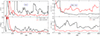 |
Fig. 3. The impact of variability. The two panels show the ideal and resistive case for MAD models (left panels) and Multi-loop models (right panels). Upper panels: Measure of the variability for the mass-accretion rate s/⟨ṁ⟩, Lower panels: Measure of the variability for the normalized magnetic flux accumulated on the black hole horizon s/⟨ϕBH⟩, both for a time window of ±270 M (Event Horizon Telescope Collaboration 2022b) (see Table 1 for details). |
The variability imprinted on the normalized magnetic flux is similar in the MAD models (left panel). More specifically, at late times (8000 − 10 000 M), it stabilizes around 0.2. The minimum variability occurs in the MAD model with η = 5 × 10⁻⁵. The intense reconnection near the horizon caused by colliding flux tubes of opposite polarity significantly increases the variability in the normalized flux in the multi-loop models (Nathanail et al. 2022b).
The mass-accretion rate is a measure of how much mass is falling onto the black hole. It plays a crucial role in shaping the radiation light curve, in particular, at 230 GHz. Studies have shown a close link between the variability in the mass-accretion rate and the variability in the light curve at 230 GHz (Porth et al. 2019; Chatterjee et al. 2021). For this reason, we primarily focused on the variability in the mass-accretion rate.
The results of the mean variability are summarized in Fig. 4 for two different time windows, namely 3000–5000 M and 8000–10 000 M. The variability is significantly reduced when resistivity is only included in the multi-loop model. For models capable of reaching the MAD state, the variability is not significantly affected by the inclusion of resistivity. However, there is no simple relation between the variability of the flow and the resistivity of the plasma, as shown in Fig. 4. A proper analysis of the 230 GHz light curve, which is the EHT target frequency, will be conducted in future studies.
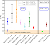 |
Fig. 4. Measure of the variability for the mass-accretion rate s/⟨ṁ⟩, (error bars ±1 s) for all MAD and multi-loop models in time windows 3000 − 5000 M (dashed error bars) and 8000 − 10 000 M (solid error bars) respectively. |
3. Conclusions
Our key findings are listed below.
-
For MAD models, a resistivity of η = 5 × 10⁻⁵ − 10−6 only affect the variability of the flow very little, indicating that the dynamics are primarily driven by magnetic flux eruption events.
-
For MAD models, simulations with a resistivity of η = 5 × 10⁻³ − 10−4 show significant magnetic field diffusion into the disk. This hinders the efficient accumulation of magnetic flux from the accretion flow.
-
Even when frequent reconnection events lead to an increased variability in the magnetic flux accumulation, the resistivity in multi-loop models significantly reduces the variability in the accretion flow. We stress that we did not expect the resistivity to have this effect.
Data availability
The data underlying this article will be shared on reasonable request to the corresponding author.
For Sgr A*, and a magnetic field of B ≈ 30 G, resistivity is η = ηcode × tg s, thus  s in Gaussian/ESU units, for reference this value is well above the Spitzer resistivity (ηSP = 1.15 × 10⁻¹⁴ Z lnΛ(T)−3/2 ≈ 10−20 s, with Z = 1 for hydrogen, lnΛ the Coulomb logarithm and T the electron temperature) of the local plasma, but closer to the expected anomalous resistivity expected in astrophysical accretion disks.
The time window was chosen to cover 3 hours of observational data for Sgr A* (see Event Horizon Telescope Collaboration 2022b for details).
The variability for all MAD models is shown in Appendix B.
Acknowledgments
Support comes from the ERC Advanced Grant “JETSET: Launching, propagation and emission of relativistic jets from binary mergers and across mass scales” (Grant No. 884631). YM is supported by the National Key R&D Program of China (grant no. 2023YFE0101200), the National Natural Science Foundation of China (grant no. 12273022), and the Shanghai municipality orientation program of basic research for international scientists (grant no. 22JC1410600). CMF is supported by the DFG research grant “Jet physics on horizon scales and beyond” (Grant No. 443220636) within the DFG research unit “Relativistic Jets in Active Galaxies” (FOR 5195). ACO gratefully acknowledges “Ciencia Básica y de Frontera 2023-2024” program of the “Consejo Nacional de Humanidades, Ciencias y Tecnología” (CONAHCYT, Mexico) project CBF2023-2024-1102 and SNI 257435. This work was supported by computational time granted from the National Infrastructures for Research and Technology S.A. (GRNET S.A.) in the National HPC facility - ARIS - under project ID 16033. Simulations were performed also on SuperMUC at LRZ in Garching, on the GOETHE-HLR cluster at CSC in Frankfurt, and on the HPE Apollo Hawk at the High Performance Computing Center Stuttgart (HLRS).
References
- Baganoff, F. K., Bautz, M. W., Brandt, W. N., et al. 2001, Nature, 413, 45 [Google Scholar]
- Bhattacharjee, A., Huang, Y.-M., Yang, H., & Rogers, B. 2009, Phys. Plasmas, 16, 112102 [Google Scholar]
- Bisnovatyi-Kogan, G. S., & Ruzmaikin, A. A. 1974, Ap&SS, 28, 45 [NASA ADS] [CrossRef] [Google Scholar]
- Broderick, A. E., Gold, R., Georgiev, B., et al. 2022, ApJ, 930, L21 [NASA ADS] [CrossRef] [Google Scholar]
- Burke, C. J., Shen, Y., Blaes, O., et al. 2021, Science, 373, 789 [NASA ADS] [CrossRef] [Google Scholar]
- Chashkina, A., Bromberg, O., & Levinson, A. 2021, MNRAS, 508, 1241 [NASA ADS] [CrossRef] [Google Scholar]
- Chatterjee, K., Markoff, S., Neilsen, J., et al. 2021, MNRAS, 507, 5281 [NASA ADS] [CrossRef] [Google Scholar]
- Cruz-Osorio, A., Fromm, C. M., Mizuno, Y., et al. 2022, Nat. Astron., 6, 103 [NASA ADS] [CrossRef] [Google Scholar]
- Del Zanna, L., Zanotti, O., Bucciantini, N., & Londrillo, P. 2007, A&A, 473, 11 [NASA ADS] [CrossRef] [EDP Sciences] [Google Scholar]
- Del Zanna, L., Papini, E., Landi, S., Bugli, M., & Bucciantini, N. 2016, MNRAS, 460, 3753 [Google Scholar]
- Doeleman, S. S., Weintroub, J., Rogers, A. E. E., et al. 2008, Nature, 455, 78 [NASA ADS] [CrossRef] [Google Scholar]
- Event Horizon Telescope Collaboration (Akiyama, K., et al.) 2019a, ApJ, 875, L1 [Google Scholar]
- Event Horizon Telescope Collaboration (Porth, O., et al.) 2019b, ApJS, 243, 26 [NASA ADS] [CrossRef] [Google Scholar]
- Event Horizon Telescope Collaboration (Akiyama, K., et al.) 2021, ApJ, 910, L13 [Google Scholar]
- Event Horizon Telescope Collaboration (Akiyama, K., et al.) 2022a, ApJ, 930, L12 [NASA ADS] [CrossRef] [Google Scholar]
- Event Horizon Telescope Collaboration (Akiyama, K., et al.) 2022b, ApJ, 930, L16 [NASA ADS] [CrossRef] [Google Scholar]
- Event Horizon Telescope Collaboration (Akiyama, K., et al.) 2024, ApJ, 964, L26 [CrossRef] [Google Scholar]
- Falcke, H., Goss, W. M., Matsuo, H., et al. 1998, ApJ, 499, 731 [NASA ADS] [CrossRef] [Google Scholar]
- Fishbone, L. G., & Moncrief, V. 1976, ApJ, 207, 962 [NASA ADS] [CrossRef] [Google Scholar]
- Fromm, C. M., Cruz-Osorio, A., Mizuno, Y., et al. 2022, A&A, 660, A107 [NASA ADS] [CrossRef] [EDP Sciences] [Google Scholar]
- Genzel, R., Schödel, R., Ott, T., et al. 2003, Nature, 425, 934 [NASA ADS] [CrossRef] [Google Scholar]
- Georgiev, B., Pesce, D. W., Broderick, A. E., et al. 2022, ApJ, 930, L20 [NASA ADS] [CrossRef] [Google Scholar]
- Guo, F., Liu, Y.-H., Daughton, W., & Li, H. 2015, ApJ, 806, 167 [NASA ADS] [CrossRef] [Google Scholar]
- Hada, K., Kino, M., Doi, A., et al. 2013, ApJ, 775, 70 [Google Scholar]
- Igumenshchev, I. V. 2008, ApJ, 677, 317 [NASA ADS] [CrossRef] [Google Scholar]
- Igumenshchev, I. V., Narayan, R., & Abramowicz, M. A. 2003, ApJ, 592, 1042 [Google Scholar]
- Jiang, H.-X., Mizuno, Y., Fromm, C. M., & Nathanail, A. 2023, MNRAS, 522, 2307 [NASA ADS] [CrossRef] [Google Scholar]
- Jiang, H.-X., Mizuno, Y., Dihingia, I. K., et al. 2024, A&A, 688, A82 [NASA ADS] [CrossRef] [EDP Sciences] [Google Scholar]
- Kalapotharakos, C., Harding, A. K., Kazanas, D., & Contopoulos, I. 2012, ApJ, 754, L1 [Google Scholar]
- Kim, J., Marrone, D. P., Roy, A. L., et al. 2018, ApJ, 861, 129 [NASA ADS] [CrossRef] [Google Scholar]
- Li, J., Spitkovsky, A., & Tchekhovskoy, A. 2012, ApJ, 746, 60 [Google Scholar]
- Mahlmann, J. F., Levinson, A., & Aloy, M. A. 2020, MNRAS, 494, 4203 [Google Scholar]
- Mattia, G., Del Zanna, L., Bugli, M., et al. 2023, A&A, 679, A49 [NASA ADS] [CrossRef] [EDP Sciences] [Google Scholar]
- Mizuno, Y., Younsi, Z., Fromm, C. M., et al. 2018, Nat. Astron., 2, 585 [Google Scholar]
- Narayan, R., Igumenshchev, I. V., & Abramowicz, M. A. 2003, PASJ, 55, L69 [NASA ADS] [Google Scholar]
- Nathanail, A., Porth, O., & Rezzolla, L. 2019, ApJ, 870, L20 [NASA ADS] [CrossRef] [Google Scholar]
- Nathanail, A., Fromm, C. M., Porth, O., et al. 2020a, MNRAS, 495, 1549 [Google Scholar]
- Nathanail, A., Gill, R., Porth, O., Fromm, C. M., & Rezzolla, L. 2020b, MNRAS, 495, 3780 [NASA ADS] [CrossRef] [Google Scholar]
- Nathanail, A., Dhang, P., & Fromm, C. M. 2022a, MNRAS, 513, 5204 [NASA ADS] [CrossRef] [Google Scholar]
- Nathanail, A., Mpisketzis, V., Porth, O., Fromm, C. M., & Rezzolla, L. 2022b, MNRAS, 513, 4267 [NASA ADS] [CrossRef] [Google Scholar]
- Obergaulinger, M., & Aloy, M. Á. 2020, J. Phys. Conf. Ser., 1623, 012018 [Google Scholar]
- Obergaulinger, M., Cerdá-Durán, P., Müller, E., & Aloy, M. A. 2009, A&A, 498, 241 [NASA ADS] [CrossRef] [EDP Sciences] [Google Scholar]
- Olivares, H., Porth, O., Davelaar, J., et al. 2019, A&A, 629, A61 [NASA ADS] [CrossRef] [EDP Sciences] [Google Scholar]
- Pandey, B. P., & Wardle, M. 2012, MNRAS, 423, 222 [NASA ADS] [CrossRef] [Google Scholar]
- Papadopoulos, D. B., & Contopoulos, I. 2019, MNRAS, 483, 2325 [NASA ADS] [CrossRef] [Google Scholar]
- Parfrey, K., Giannios, D., & Beloborodov, A. M. 2015, MNRAS, 446, L61 [Google Scholar]
- Porth, O., Olivares, H., Mizuno, Y., et al. 2017, Comput. Astrophys. Cosmol., 4, 1 [Google Scholar]
- Porth, O., Chatterjee, K., Narayan, R., et al. 2019, ApJS, 243, 26 [Google Scholar]
- Rembiasz, T., Obergaulinger, M., Cerdá-Durán, P., Aloy, M.-Á., & Müller, E. 2017, ApJS, 230, 18 [Google Scholar]
- Ripperda, B., Bacchini, F., Porth, O., et al. 2019a, ApJS, 244, 10 [NASA ADS] [CrossRef] [Google Scholar]
- Ripperda, B., Porth, O., Sironi, L., & Keppens, R. 2019b, MNRAS, 485, 299 [CrossRef] [Google Scholar]
- Ripperda, B., Bacchini, F., & Philippov, A. A. 2020, ApJ, 900, 100 [NASA ADS] [CrossRef] [Google Scholar]
- Satapathy, K., Psaltis, D., Özel, F., et al. 2022, ApJ, 925, 13 [NASA ADS] [CrossRef] [Google Scholar]
- Selvi, S., Porth, O., Ripperda, B., et al. 2023, ApJ, 950, 169 [NASA ADS] [CrossRef] [Google Scholar]
- Siegel, D. M., Ciolfi, R., Harte, A. I., & Rezzolla, L. 2013, Phys. Rev. D, 87, 121302 [NASA ADS] [CrossRef] [Google Scholar]
- Takahashi, R. 2008, MNRAS, 383, 1155 [Google Scholar]
- Tchekhovskoy, A., Narayan, R., & McKinney, J. C. 2011, MNRAS, 418, L79 [NASA ADS] [CrossRef] [Google Scholar]
- Uzdensky, D. A., Loureiro, N. F., & Schekochihin, A. A. 2010, Phys. Rev. Lett., 105, 235002 [Google Scholar]
- Yuan, Y., Blandford, R. D., & Wilkins, D. R. 2019a, MNRAS, 484, 4920 [NASA ADS] [CrossRef] [Google Scholar]
- Yuan, Y., Spitkovsky, A., Blandford, R. D., & Wilkins, D. R. 2019b, MNRAS, 487, 4114 [NASA ADS] [CrossRef] [Google Scholar]
Appendix A: Appendix A. Magnetic field accumulation in Resistive MAD simulations
To better understand the dependence of simulation results on resistivity, Fig. A.1 shows the average normalized magnetic flux on the horizon for all MAD models. The averages are taken over two-time windows: 3000 − 5000 M and 3000 − 10000 M. The figure clearly shows the flaring event for model MAD.S.26.E.−4, where the flux fluctuates near the MAD limit in the first window and then drops slightly. Model MAD.S.26.E.−3 shows a substantially lower flux already in the first window, indicating a clear deviation from typical MAD behavior. Longer simulations could highlight
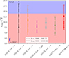 |
Fig. A.1. The mean normalized magnetic flux accumulated on the black-hole horizon (error bars indicate ±1s) for all MAD models in time windows 3000 − 5000 M (dashed error bars) and 3000 − 10000 M (solid error bars) respectively. The dashed horizontal line depicts the MAD saturation value |
Resistivity significantly impacts magnetic flux accumulation in MAD simulations due to energy dissipation at the edge of the magnetized funnel. Models with a rather low resistivity (η = 5 × 10⁻⁵) exhibit a behavior consistent with standard MAD models. At the highest resistivity run MAD.S.26.E.−3 the system settles quickly into a state with very low magnetic flux on the horizon (see left, upper and bottom panels of Fig 2).
The effect of numerical resolution was compared in two simulations with η = 5 × 10⁻⁵, where the high-resolution run is indicated as HR, MAD.S.26.E.−5.HR’. The higher resolution allows for a more accurate representation of small-scale physical processes, such as reconnection events at current sheets. As a consequence, the HR simulation exhibits more efficient magnetic energy dissipation near the edge of the funnel, resulting in a lower average accumulated flux compared to the standard resolution simulations. However, a definitive conclusion on the quantitative impact of resolution would require running the HR simulations for a longer time to ensure we capture the behavior of the system till 10000 M. In general, longer simulations could highlight whether our results remain consistent or change over extended time evolution.
Models with η = 5 × 10⁻⁶, suggest that a stronger initial magnetic field (in cyan, initial β = 26) allows the system to accumulate more flux faster and reach a state closer to the ideal MAD limit even in the presence of some resistivity. This comment must be the same for all models, meaning that initialization with higher σ will eventually bring more magnetic flux at the event horizon. The simulations reveal that resistivity plays a crucial role in magnetic flux accumulation. Lower resistivity allows for behavior consistent with the standard MAD model. However, as resistivity increases, dissipation processes become more prominent, leading to flare events and a significant reduction in the accumulated magnetic flux.
Appendix B: Appendix B. Variability for all MAD models
In this Appendix we provide details for the variability of all MAD models in our study. Fig. B.1 presents the results for s/⟨ṁ⟩ (upper panel) and s/⟨ϕBH⟩ (lower panel) for a time window of ±270 M (Event Horizon Telescope Collaboration 2022b).
 |
Fig. B.1. Upper panels: the measure of variability for the mass accretion rate s/⟨ṁ⟩, Lower panels: the measure of variability for the normalized magnetic flux accumulated on the black-hole horizon s/⟨ϕBH⟩, both for a time window of ±270 M (Event Horizon Telescope Collaboration 2022b) for all MAD models ideal and with different resistivity (see Table 1 for details.) |
The model with the highest resistivity of η = 5 × 10⁻³ (MAD.S.26.E.−3, blue line), exhibits a large bump at early times ( 3000 − 3500 M) likely corresponding to a rapid loss of magnetic flux. This is followed by a minimum variability state, which then steadily increases until the end of the simulation. Model MAD.S.26.E.−4, which has a lower resistivity (η = 5 × 10⁻⁴, orange line) shows a similar initial variability bump and continues to exhibit recurring bumps every 1000 − 2000 M.
As is seen in models MAD.S.26.E.−5 and MAD.S.26.E.−5.HR, higher resolution reduces the numerical diffusion and let only the physical resistivity to act. Another point to make for the HR run is that it reduces slightly the variability in the first window, this was expected since having HR will impact any variability imposed from reconnection events. Further reducing the resistivity to η = 5 × 10⁻⁶, results in a similar level of variability to the standard ideal MAD model.
Appendix C: Appendix C. Variability of the Power of the jet
In this appendix we explore the variability on the jet power. For the multi-loop models such discussion does not make much sense, since it has been shown that there is no production of a steady jet (Nathanail et al. 2020a). Multi-loop models exhibit periodic outbursts either from the upper or the lower hemisphere. Thus, the variability of the jet power will be discussed only for MAD models.
The power is measured through the energy flux that passes through a 2-sphere placed at 50 rg. It is defined as follows:
where the integrand in (C.1) is set to zero everywhere on the integrating surface where σ ≤ 1, in order to account only for the jet component.
The power of the jet of four MAD models is shown in the upper panel of Fig. C.1. The ideal MAD model, MAD.S.100.E.00, has a similar power output with the low resistivity model, MAD.S.100.E.−6. However, when the resistivity increases significantly the picture vastly changes. For models MAD.S.26.E.−3 and MAD.S.26.E.−4, there is an initial jump at the normalized magnetic flux at around 2500 M (see Fig. 2). A similar behavior is seen in the jet power, with an early burst followed by a steady decline in power throughout the simulation time.
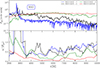 |
Fig. C.1. Upper panels: The power of the jet as defined in Eq. (C.1) in code units. Lower panel: the measure of variability for the jet power for four representative MAD models. |
To measure the variability in the jet power we make use of Eq. (5), where ki = Pjet in this case. The ideal model shows the smallest variability on the jet power, whereas all the rest resistive models, shown in the lower panel of Fig. C.1, exhibit larger variability.
Appendix D: Appendix D. MRI quality factor Qθ
We provide here the definition of the MRI quality factor Qθ and details on its calculation presented in Table 1. We evaluate the so-called “quality factor” Qθ, in terms of the ration between the grid spacing in a given direction Δxθ, (e.g., the θ-direction) and the wavelength of the fastest growing MRI mode in that direction (i.e., λθ), where both quantities are evaluated in the tetrad basis of the fluid frame  (see Takahashi 2008; Siegel et al. 2013; Porth et al. 2019, for details)

where
Ω := uϕ/ut is the angular velocity of the fluid and the corresponding grid resolution is  . Finally the average of Qθ is done in space and time, specifically in a time window of 200 M and spatially in the region of interest at angles 60o < θ < 120o and r < 40 rg, inside the heart of the disk.
All Tables
All Figures
|
Fig. 1. Dynamics of the accretion flow. The two panels show the ideal and resistive case for MAD models (left panels) and Multi-loop models (right panels). Upper panels: Mass accretion rate, Ṁ, through the black hole horizon. Middle panels: Magnetic flux accumulated on the black hole horizon, ΦBH. Lower panels: Normalized magnetic flux accumulated on the black hole horizon, ϕBH (see Table 1 for model details). |
| In the text | |
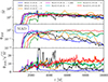 |
Fig. 2. Same as Fig. 1 for all MAD models (see Table 1 for details). |
| In the text | |
|
Fig. 3. The impact of variability. The two panels show the ideal and resistive case for MAD models (left panels) and Multi-loop models (right panels). Upper panels: Measure of the variability for the mass-accretion rate s/⟨ṁ⟩, Lower panels: Measure of the variability for the normalized magnetic flux accumulated on the black hole horizon s/⟨ϕBH⟩, both for a time window of ±270 M (Event Horizon Telescope Collaboration 2022b) (see Table 1 for details). |
| In the text | |
|
Fig. 4. Measure of the variability for the mass-accretion rate s/⟨ṁ⟩, (error bars ±1 s) for all MAD and multi-loop models in time windows 3000 − 5000 M (dashed error bars) and 8000 − 10 000 M (solid error bars) respectively. |
| In the text | |
|
Fig. A.1. The mean normalized magnetic flux accumulated on the black-hole horizon (error bars indicate ±1s) for all MAD models in time windows 3000 − 5000 M (dashed error bars) and 3000 − 10000 M (solid error bars) respectively. The dashed horizontal line depicts the MAD saturation value |
| In the text | |
|
Fig. B.1. Upper panels: the measure of variability for the mass accretion rate s/⟨ṁ⟩, Lower panels: the measure of variability for the normalized magnetic flux accumulated on the black-hole horizon s/⟨ϕBH⟩, both for a time window of ±270 M (Event Horizon Telescope Collaboration 2022b) for all MAD models ideal and with different resistivity (see Table 1 for details.) |
| In the text | |
|
Fig. C.1. Upper panels: The power of the jet as defined in Eq. (C.1) in code units. Lower panel: the measure of variability for the jet power for four representative MAD models. |
| In the text | |
Current usage metrics show cumulative count of Article Views (full-text article views including HTML views, PDF and ePub downloads, according to the available data) and Abstracts Views on Vision4Press platform.
Data correspond to usage on the plateform after 2015. The current usage metrics is available 48-96 hours after online publication and is updated daily on week days.
Initial download of the metrics may take a while.