© The Authors 2025

1. Introduction

The solar corona is the outermost layer of the sun and its dynamic is governed by the influence of the magnetic field. Various phenomena occur in the solar corona, such as coronal heating, mass ejections, prominences, flares, and sigmoidal structures, which require a better understanding of the structure and strength of the solar coronal magnetic field (Gary 2001; Priest 2014; Wiegelmann et al. 2014; Mackay et al. 2016; Aschwanden 2019). The data obtained by observations and tracking of spacecraft such as Solar Dynamics Observatory (SDO), TRACE, and Yohkoh have enabled the solar physicist to understand the working mechanisms of the magnetic field in solar coronal dynamics (Nakariakov et al. 1999; Berghmans & Clette 1999; De Moortel et al. 2000; Aschwanden et al. 1999; Wang et al. 2003; Wang & Solanki 2004; Sun et al. 2012; Chintzoglou & Zhang 2013). Nevertheless, the coronal spectral lines are optically thin, and due to low light intensity, the long-standing problem of measurement of the magnetic field still poses a challenge (Ruderman et al. 2008; Verth & Erdélyi 2008; Van Doorsselaere et al. 2008; Altschuler et al. 1977; Altschuler & Newkirk 1969; Yang et al. 2020a). Lin et al. (2004) demonstrated that the magnetic field can be measured using the Zeeman effect, but interpreting these coronal lines is highly complex due to line-of-sight complications. As an alternative to direct measurements, methods have been developed to utilise observed magnetic fields in the photosphere to infer properties of the solar corona. These methods do not consider thermal pressure and gravity forces, and employ a force-free magnetic field model where electric currents run parallel to magnetic field lines (Grad & Rubin 1958; Amari et al. 1999, 1997; Schrijver et al. 2006; Wiegelmann et al. 2006). In addition to the effort done for magnetic field reconstructions, some semi-analytical models for the coronal magnetic field over active regions were introduced by Low & Lou (1990) (L&L) and Čadež (2005). Wheatland et al. (2000) utilised the semi-analytical model proposed by Low & Lou (1990) to reconstruct the magnetic field using an artificial magnetogram for an active region through an optimisation mechanism. This optimisation technique was developed later by Wiegelmann (2004) and Wiegelmann et al. (2005b, 2012). Nasiri & Wiegelmann (2019) and Fatholahzadeh et al. (2023) employed the Lagrange multiplier technique to reconstruct the magnetic field of the solar corona. The corresponding results are consistent with those obtained by other optimisation methods. Despite the difficulties in direct observation, valuable information about physical quantities of the solar corona has been extracted through seismological studies, where a theoretical model is considered and compared with observational data (Edwin & Roberts 1983, 1988; Roberts et al. 1984; Goossens et al. 1992; Mikić et al. 1999; Verwichte et al. 2004; Aschwanden 2005).

Recent research into wave phenomena in the solar atmosphere indicates that transverse oscillations and Alfvénic motions play a significant role in coronal heating. One study, Bate et al. (2022), investigates transverse oscillations in umbral fibrils in a strongly magnetised sunspot, revealing that these oscillations carry a substantial energy flux of 7.52×10⁻²⁶ W m⁻², which is three to four orders of magnitude greater than the energy loss rate of plasma in active regions. These oscillations continuously transfer energy from the sunspot to the plasma confined in larger coronal loops, potentially contributing to coronal heating.

Another study, Skirvin et al. (2023), examines Alfvénic motions arising from asymmetric acoustic wave drivers, demonstrating how an acoustic driver can produce transverse oscillations in magnetic loops. Three-dimensional magnetohydrodynamic (MHD) simulations reveal that these motions are significant due to the breaking of azimuthal symmetry and can enhance our understanding of wave behaviour in solar structures.

Additionally, high-frequency oscillations in chromospheric spicules have been highlighted by Petrova et al. (2023), showing that their amplitude and velocity change with height, which may aid energy transfer within the solar atmosphere. Observations of high-frequency transverse motions in coronal loops also indicate significant energy fluxes that could contribute to coronal heating. The results indicate that high-frequency transverse motions observed in small coronal loops consist of two types of transverse motions: one with a period of 14 seconds and another with a period of 30 seconds (Petrova et al. 2023). The velocity amplitudes for the shorter and longer oscillations are estimated to be 72 km/s and 125 km/s, respectively. Energy flux calculations show that the energy flux for the 14-second oscillation is approximately 1.9 kW/m², while for the 30-second oscillation it is around 6.5 kW/m². These values suggest that these oscillations could serve as a significant energy source for coronal heating and lend further credibility to coronal heating models based on wave damping.

Hasan & Sobouti (1987) explored the modal structure of a polytropic star with a uniform magnetic field. Nasiri (1992) followed the same problem for a funnel-shaped flux tube with a variable cross section introducing some level of magnetic field inhomogeneity. The use of oscillation theory has been employed to find the magnetic field in the solar corona (Chen 2015; Jess et al. 2016; Yang et al. 2020b; Petrie 2024; Nakariakov & Ofman 2001), but conversely, the issue of examining coronal oscillations with the reconstructed magnetic field has not been addressed. Our aim in this paper is to focus on this topic. We used the L&L semi-analytical model to obtain an artificial magnetogram and assume the computational box over an active region on this magnetogram. Furthermore, we optimised the magnetic field using the Lagrange multiplier technique. We followed the Hassan-Sobouti mathematical procedure to obtain the modal frequencies of transverse oscillations. In the next section, we describe the techniques used for the reconstruction of the magnetic field and the corresponding numerical method is presented. In Sect. 3, the dynamical equations and oscillatory modes are studied. The numerical method and results are presented in Sect. 4, and Sect. 5 is devoted to conclusions.

2. Reconstruction of the magnetic field

In a coronal plasma, the strength and structure of the magnetic field are not precisely quantified due to the weak Zeeman splitting phenomena. Consequently, reconstruction of the magnetic field within the solar corona is employed using extrapolation methods and leveraging available magnetic data. Such reconstructions primarily draw from magnetograms directly measured on the solar photosphere. Several models and methodologies have been developed to aid these reconstructions, assuming that the coronal dynamics are governed by the force-free magnetic fields. The force-free and divergence-free conditions for the magnetic field (B) are

$$(\nabla \times B)\times B=0,$$(1)

where B≡B(x,y,z,t), and

$$\nabla ·B=0.$$(2)

The solution of the above equations is

$$\nabla \times B=\alpha (\text{r})B,$$(3)

where the force-free parameter, α(r), is a scalar function determining the degree of the force-free condition of the magnetic field. For potential field (current-free), α(r) is zero; for linear force-free fields, it remains constant; and for non-linear force-free fields, it is a function of spatial coordinates.

2.1. Review of optimisation methods

Obtaining a general solution for Eq. (1) is not feasible. To address this challenge, a semi-analytical solution known as the L&L method was proposed by Low & Lou (1990). In addition to the analytical solutions, the numerical methods were developed by Grad & Rubin (1958), Wheatland et al. (2000), Schrijver et al. (2006), Wiegelmann et al. (2006, 2014, 2017). The Wheatland et al. (2000) force-free magnetic field model (WSR) aims to minimise a function that incorporates the magnetic field and its derivatives as follows:

$$L_{\mathrm{WSR}}={\displaystyle {{\displaystyle \int }}_v}\mathrm{d}v\left((|B{|}^{-2}(\nabla \times B)\times B{)}^2+|\nabla ·B{|}^2\right),$$(4)

where L_WSR is the Lagrangian of Wheatland, Sturrock, and Roumeliotis (Wheatland et al. 2000), and v represents the volume of the computational box. Equation (4) is positive and converges to its minimum value if its variation with the iteration parameter, t, is negative:

$$\frac{\mathrm{d}{L}_{\mathrm{WSR}}}{\mathrm{d}t}<0.$$(5)

To ensure the condition of Eq. (5), one may take the derivative of Eq. (4) and use appropriate vector algebra to obtain

$$\begin{array}{c}\frac{1}{2}\frac{\partial L_{\mathrm{WSR}}}{\partial t}={{\displaystyle \int }}_v\left(\frac{\partial B}{\partial t}·F_{\mathrm{WSR}}\right)\mathrm{d}v+{{\displaystyle \int }}_s\left(\frac{\partial B}{\partial t}·G_{\mathrm{WSR}}\right)\mathrm{d}s,\hfill \end{array}$$(6)

where F_WSR is a function of the magnetic field as follows:

$$\begin{array}{cc}\hfill F_{\mathrm{WSR}}& =\nabla \times ({\mathbf{\Omega }}_{\mathrm{WSR}}\times B)-{\mathbf{\Omega }}_{\mathrm{WSR}}\times (\nabla \times B)\hfill \\ \hfill & -\nabla ({\mathbf{\Omega }}_{\mathrm{WSR}}·B)+{\mathbf{\Omega }}_{\mathrm{WSR}}(\nabla ·B)+{\mathrm{\Omega }}_{\mathrm{WSR}}^{2}B\hfill \end{array}$$(7)

and

$$G_{\mathrm{WSR}}=\hat{n}\times ({\mathbf{\Omega }}_{\mathrm{WSR}}\times B)-\hat{n}({\mathbf{\Omega }}_{\mathrm{WSR}}·B),$$(8)

where

$${\mathbf{\Omega }}_{\mathrm{WSR}}=B^{-2}[(\nabla \times B)\times B-(\nabla ·B)B].$$(9)

Assuming

$${\left(\frac{\partial B}{\partial t}\right)}_v=-\mu F_{\mathrm{WSR}},$$(10)

where μ is a positive parameter to be specified during numeric calculation, and letting the surface integral that appears in Eq. (6) vanish by considering the condition

$${\left(\frac{\partial B}{\partial t}\right)}_s=0,$$(11)

one gets the following equation:

$$\frac{\mathrm{d}{L}_{\mathrm{WSR}}}{\mathrm{d}t}=-2\int \mathrm{d}v{F}_{\mathrm{WSR}}^2.$$(12)

Equation (6) shows that L_WSR is a decreasing function of the iteration parameter, in agreement with Eq. (5). This means that the magnetic field remains constant on the surface, s, during the iteration process. One may solve Eq. (10) by an iteration procedure, and using a potential field as an input magnetic field, both terms in the integral tend towards zero, confirming the force-free condition and solenoidal nature of the magnetic field, respectively. Nasiri & Wiegelmann (2019) modified this model using a scalar Lagrange multiplier function as a constraint optimisation method (COS). Their proposed functional was

$$L_{\mathrm{COS}}={\displaystyle {\int }_v}\mathrm{d}v({\lambda }_{\mathrm{COS}}(\nabla ·B)+|B{|}^{-2}((\nabla \times B)\times B{)}^2),$$(13)

where λ_COS≡λ_COS(x,y,z,t). Taking the derivative of Equation (13) one gets:

$$\begin{array}{c}\frac{1}{2}\frac{\partial L_{\mathrm{COS}}}{\partial t}={\int }_v\frac{\partial B}{\partial t}·F_{\mathrm{COS}}\mathrm{d}v+{\int }_s\frac{\partial B}{\partial t}·G_{\mathrm{COS}}\mathrm{d}s\hspace{0.5em}+{\int }_v\frac{\partial \lambda }{\partial t}{H}_{\mathrm{COS}}\mathrm{d}v,\hfill \end{array}$$(14)

where

$$\begin{array}{c}{F}_{\mathrm{COS}}=\nabla \times ({\mathbf{\Omega }}_{\mathrm{COS}}\times B)-{\mathbf{\Omega }}_{\mathrm{COS}}\times (\nabla \times B)+\hfill \\ \hfill \\ {\mathrm{\Omega }}_{\mathrm{COS}}^{2}B+\frac{1}{2}\nabla {\lambda }_{\mathrm{COS}},\hfill \end{array}$$(15)

and

$$G_{\mathrm{COS}}=\hat{n}\times ({\mathbf{\Omega }}_{\mathrm{COS}}\times B)+\frac{1}{2}\hat{n}{\lambda }_{\mathrm{COS}},$$(16)

where

$${\mathbf{\Omega }}_{\mathrm{COS}}={\mathbf{\Omega }}_{\mathrm{WSR}}+\frac{B}{|B{|}^2}\nabla ·B.$$(17)

In this method, we have the following iterative relations for the Lagrange multiplier and magnetic field:

$${\left(\frac{\partial {\lambda }_{\mathrm{COS}}}{\partial t}\right)}_v=-{\mu }_1{H}_{\mathrm{COS}},{\left(\frac{\partial B}{\partial t}\right)}_v=-{\mu }_2{F}_{\mathrm{COS}},$$(18)

where μ₁ and μ₂ are positive parameters to be specified during numeric calculations, and

$$H_{\mathrm{COS}}=\nabla ·B.$$(19)

Assuming the following expression as input,

$${\lambda }_{\mathrm{COS}}=\nabla ·B,$$(20)

one may solve Eq. (18) iteratively.

Fatholahzadeh et al. (2023) developed the above model using the vector Lagrange multiplier function (COV), assuming the following functional:

$$L_{\mathrm{COV}}={\displaystyle {\int }_v}\mathrm{d}v(|\nabla ·B{|}^2+{\lambda }_{\mathrm{COV}}.((\nabla \times B)\times B)).$$(21)

Taking the derivative of Eq. (21) and using appropriate vector algebra, one may obtain

$$\begin{array}{cc}\frac{1}{2}\frac{\partial L_{\mathrm{COV}}}{\partial t}\hfill & ={\int }_v\left(\frac{\partial B}{\partial t}·F_{\mathrm{COV}}\right)\mathrm{d}v+{\int }_s\left(\frac{\partial B}{\partial t}·G_{\mathrm{COV}}\right)\mathrm{d}s\hfill \\ \hfill & \hfill \\ \hfill & +{\int }_v\left(\frac{\partial \lambda }{\partial t}·H_{\mathrm{COV}}\right)\mathrm{d}v,\hfill \end{array}$$(22)

where λ_COV≡λ_COV(x,y,z,t) represents the vector Lagrange multiplier, and

$$F_{\mathrm{COV}}=\nabla \times (B\times {\lambda }_{\mathrm{COV}})+(\nabla \times B)\times {\lambda }_{\mathrm{COV}}-2\nabla (\nabla ·B),$$(23)

$$H_{\mathrm{COV}}=(\nabla \times B)\times B,$$(24)

and

$$G_{\mathrm{COV}}=2(\nabla ·B)\hat{n}+(B\times {\lambda }_{\mathrm{COV}})\times \hat{n}.$$(25)

Now, the iterative equation for λ_COV and B becomes

$${\left(\frac{\partial {\lambda }_{\mathrm{COV}}}{\partial t}\right)}_v=-{\mu }_1{H}_{\mathrm{COV}}\hspace{0.5em},{\left(\frac{\partial B}{\partial t}\right)}_v=-{\mu }_2{F}_{\mathrm{COV}},$$(26)

where μ₁ and μ₂ are positive parameters to be specified during numeric calculations, and, assuming the initial value of λ_COV to be

$${\lambda }_{\mathrm{COV}}=|B{|}^{-2}((\nabla \times B)\times B),$$(27)

Equation (26) can be solved to obtain the appropriate magnetic field.

2.2. Reconstruction of magnetic field by the COV method

Despite the limitations that some authors consider for the extrapolation of force-free magnetic fields in the solar corona (Peter et al. 2015), it is believed that the results obtained from the force-free field reconstructions align well with the observations of coronal loops and active regions. Furthermore, the free magnetic energy obtained by these reconstructions is often correlated with flare activities and explains the corresponding energy storage mechanisms. Therefore, to this extent, the results obtained by reconstruction models can still be reliable and in agreement with observational data.

The nonlinear force-free field reconstruction methods that are widely used to analyse photospheric magnetic fields typically require a reference magnetic field to evaluate the force-free state of the reconstructed field. To do this, one may use a photospheric real or artificial magnetogram. The artificial magnetogram can be obtained by the semi-analytical solutions presented by Low & Lou (1990) (L&L). They derived a class of axisymmetric non-linear force-free fields which were singular at the origin. One may remove the singularity by burying the point source beneath the photosphere by depth, l, and inclining the axes of symmetry of the fields to the normal by φ. The magnetic field is obtained for the parameters φ=π/8 and l = 0.5, and the corresponding artificial magnetogram is constructed (Fig. 1). In the next step, a computational box is accomplished with dimensions of 160×160×160 grid points on this magnetogram as its lower base. The distance between the centre to centre of each neighbouring grid point in the x,y, and z directions is considered to be 720 km, according to SHO/HMI images (Wiegelmann et al. 2005a). The boundaries are preserved with a potential field, and the magnetic field inside the box is reconstructed using the COV optimisation method. To achieve this, one may use Eq. (21) to minimise L_COV using an iterative mechanism. As shown in Fig. 2, L_COV converges towards zero, indicating that both positive terms in Eq. (21) approach zero. We performed 6000 iteration steps, starting with a potential field and, finally, we obtain an almost non-linear force-free magnetic field such that the angle between the magnetic field and electric current density vectors reaches a value of 7.647° (Fig. 3). The corresponding reconstructed magnetic field is shown in Fig. 4.

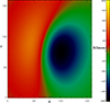Fig. 1. Artificial magnetogram of dimensions 160×160, obtained by the L&L method with parameters φ=π/8 and l = 0.5, with colour code in Gauss.

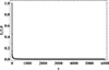Fig. 2. Behaviour of $\frac{L}{L_0}$ over 6000 iteration steps. L0 is the Lagrangian at the beginning of the iteration.

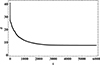Fig. 3. Angle (θ) between the magnetic field and electric current density vector, which reaches 7.647 with 6000 iteration steps.

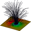Fig. 4. Reconstruction of 3D magnetic fields for the box of dimensions 160 × 160 × 160 gridpoints.

The iterative behaviour of λ_COV is plotted in Fig. 5, which shows the convergence of λ_COV to its maximum value. To normalise the graph in Fig. 5, we divided each value of lambda in different iterations by the maximum value of lambda, which is the highest value of lambda across all iterations. To ensure the accuracy of the results, we examined the following indicators defined by Schrijver et al. (2006).

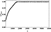Fig. 5. Behaviour of λ versus iteration parameter. λmax is the maximum value of lambda in the last iteration.

(A) Relative magnetic energy (RME):

RME is defined as the ratio of the reconstructed to the calculated magnetic field energies:

$$\mathrm{RME}\equiv \frac{{\sum }_{i=1}^N|B_i{|}^2}{{\sum }_{i=1}^N|b_i{|}^2},$$(28)

where B_i is the final non-linear force-free field, b_i is the corresponding L&L semi-analytical solution, and N denotes the total number of grid points in the computational box.

(B) Mean vector error (MVE):

MVE quantifies the average discrepancy between the reconstructed and calculated magnetic field vectors. It provides an overall measure of reconstruction accuracy but is insensitive to the direction of vectors. It is defined as

$$\mathrm{MVE}\equiv \frac{1}{N}{\displaystyle \sum _{i=1}^N}\frac{|B_i-b_i|}{|b_i|},$$(29)

and MVE approaches zero when b_i and B_i are almost identical.

(C) Vector correlation (VC):

VC is defined as

$$\mathrm{VC}\equiv \frac{{\sum }_{i=1}^N(B_i·b_i)}{\sqrt{{\sum }_{i=1}^N|B_i{|}^2{\sum }_{i=1}^N|b_i{|}^2}}·$$(30)

In contrast to MVE, the VC approaches unity when b_i and B_i are almost identical, as is clear from Eq. (30).

(D) Normalised vector error (NVE):

NVE is similar to MVE, but instead of using the vector magnitudes, it utilises their norms and is defined as

$$\mathrm{NVE}\equiv \frac{{\sum }_{i=1}^N|B_i-b_i|}{{\sum }_{i=1}^N|b_i|}·$$(31)

NVE is sensitive to the direction of vectors and provides additional insight into the error distribution.

(E) Cauchy-Schwartz correlation (CSC):

CSC measures the correlation between the reconstructed and calculated magnetic field vectors and is defined as

$$\mathrm{CSC}\equiv \frac{1}{N}{\displaystyle \sum _{i=1}^N}\frac{B_i·b_i}{|B_i||B_i|}·$$(32)

CSC ranges from 0 to 1, indicating no correlation and perfect correlation, respectively.

Table 1 provides a comparative analysis of the indicators associated with the L&L and COV methods. The results show that the two methods are in close agreement.

3. Dynamical equations and oscillatory modes

Hasan & Sobouti (1987) introduced a technique for studying the modal analysis and wave propagation inside a cubic-shaped flux tube embedded in a magnetic environment. They introduced a perturbation on a fluid element and decomposed the resultant disturbances into non-rotational and solenoidal components using a gauged version of the Helmholtz theorem. In the solar corona, despite the presence of a strong magnetic field, variations in thermal pressure, gravity, and density can be disregarded. Therefore, the pressure (p) and gravity (g) modes are not relevant in the study of coronal plasma oscillations. Instead, the focus lies on the toroidal (t) modes, which are identified through MHD waves. These waves do not induce any fluctuation in plasma thermal pressure or density but only cause changes in magnetic field lines. Our methodology involved considering a flux tube with a rectangular cross section, with its lower base on the solar photospheric surface containing an active region. Cartesian coordinates were adopted, with the origin placed at the corner of the box and z = 0. The field inside the tube was the reconstructed magnetic field, obtained through the COV method, while the field outside the lateral sides was assumed to be zero. In the active regions, the magnetic field, B(x,y,z), and the mass density of the coronal plasma, ρ(x,y,z), may satisfy the following relation (Priest 2014):

$$\rho (x,y,z)={\rho }_0\frac{B(x,y,z)}{B_0},$$(33)

where ρ₀ and B₀ represent the plasma density and magnetic field at z = 0, respectively.

3.1. Equations

If we consider a fluid element that is perturbed from its equilibrium state and let ξ(x,t) represent the small Lagrangian displacement of the fluid element, then using the momentum equation and the induction equation in the absence of pressure and gravitational forces, we can express them as

$$\rho \frac{{\partial }^2\xi (x,t)}{\partial t^2}=\frac{1}{4\pi }(\nabla \times \delta B)\times B,$$(34)

where

$$\delta B=\nabla \times (\xi \times B).$$(35)

Multiplying Eq. (34) by ξ^*, integrating over the entire volume and assuming ξ(r,t) = ξ(r)e^iωt, one gets

$${\omega }^2\int {\xi }^{*}·\rho \xi \hspace{0.5em}\mathrm{d}v=\frac{1}{4\pi }\int \mathrm{d}v{\xi }^{*}·[(\nabla \times \delta B)\times B].$$(36)

Integrating by parts, the right-hand side of Eq.(36) becomes

$$\begin{array}{cc}\hfill \frac{1}{4\pi }\int \mathrm{d}v{\xi }^{*}·[(\nabla \times \delta B)\times B]=\frac{1}{4\pi }\int \mathrm{d}v{\delta B}^{*}·\delta B+\hfill & \hfill \hfill \\ \hfill \frac{1}{4\pi }\int \mathrm{d}s[(\hat{n}·{\xi }^{*})(B·\delta B)-(B·\hat{n})({\xi }^{*}·\delta B)],\hfill & \hfill \hfill \end{array}$$(37)

where v represents the volume integral and s represents the surface integral. In compact form, Eq. (37) may be written as

$$W-{\omega }^{2}S=0,$$(38)

where

$$S=\int \mathrm{d}v\rho {\xi }^{*}·\xi .$$(39)

If we consider the reconstructed magnetic field in a box with volume, v, and denote its surfaces, s, as mathematically divided into two parts, s₁ and s₂, then in this case, we have

$$W=W_v+W_{s1}+W_{s2},$$(40)

where the volume integral

$$W_v=\frac{1}{4\pi }\int \mathrm{d}v{\delta B}^{*}·\delta B,$$(41)

and the surface integrals

$$W_{s1}=\frac{1}{4\pi }\int \mathrm{d}s(\hat{n}·{\xi }^{*})(B·\delta B)$$(42)

and

$$W_{s2}=-\frac{1}{4\pi }\int \mathrm{d}s(B·\hat{n})({\xi }^{*}·\delta B).$$(43)

W_s1 vanishes since B is normal to δB. W_s2 vanishes on the lateral surfaces since the normal components of the magnetic field are assumed to be zero on these sides. However, for the lower and upper sides, the contributions of W_s2 are negligible compared to the volume integral, W_v. It can be shown that, for our reconstructed magnetic field, the numerical values of ratio $\frac{W_{s2}}{W_v}$ are about 1.02×10⁻³ and 1.50×10⁻⁷ for the lower and upper sides, respectively.

3.2. Decomposition of Lagrangian displacements

If one lets the set of all displacements, ζ(x,t), which may not necessarily satisfy Eq. (38), be a part of the Hilbert space, H, with the inner product defined as

$$(\zeta (x,t),{\zeta }^{\prime }(x,t))={\displaystyle {\int }_V}\mathrm{d}v\zeta ·{\zeta }^{\prime },$$(44)

then by a suitable gauge transformation (Sobouti 1981), one gets

$$\rho \zeta (x,t)=-\rho \nabla {\chi }_p+\nabla \times A.$$(45)

Here, χ_p(x) is a scalar potential and A(x) is a divergence-free vector potential. The solenoidal vector, A, can be further divided into toroidal and poloidal components, $A=\nabla \times (\hat{k}{\chi }_g)+\nabla \times \nabla \times (\hat{k}{\chi }_t)$, where $\hat{k}$ is a unit vector along the z direction. Thus

$$\zeta ={\zeta }_p+{\zeta }_g+{\zeta }_t.$$(46)

By substituting Equation (46) into Equation (45), we get

$${\zeta }_p=-\nabla {\chi }_p,$$(47)

$${\zeta }_g=\frac{1}{\rho }\nabla \times \nabla \times (\hat{k}{\chi }_g),$$(48)

and

$${\zeta }_t=\frac{1}{\rho }\nabla \times \nabla \times \nabla \times (\hat{k}{\chi }_t).$$(49)

If we consider an actual mode of the fluid, ξ_s, which satisfies Eqs. (38)–(40), and expand it in terms of the basis set {ζ_p,ζ_g,ζ_t}, then

$${\xi }_s={\displaystyle \sum _r}{\zeta }_r{Z}_{\mathit{rs}},$$(50)

where Z_rs are proportionality constants and r,s=p,g, or t. Substituting Eq. (38) into Eqs. (39)–(40) and using the Rayleigh-Ritz variational technique to minimise the eigenvalues gives the matrix equation (Sobouti 1977)

$$\mathit{WZ}=\mathit{SZE},$$(51)

where E is a diagonal matrix whose elements are the eigenvalues ω² and Z=[Z_rs] is the matrix of the expansion coefficients (see Hasan & Sobouti 1987; Nasiri 1992). ζ_p and ζ_g are associated with rotational and solenoidal motions and are driven by pressure and gravity forces, respectively, which are absent in the present study. Thus, p and g modes are not excited in the flux tube and the coupling between t modes with p and g modes does not happen, giving pure toroidal motions. Toroidal modes are better represented in cylindrical coordinates, and, under the conditions of our problem, they predominantly manifest as transverse modes (Morton 2023). The elements of W and S are given in Sect. 4.

3.3. Ansatz for t motions

As outlined before, we reconstructed the magnetic field in the computational box of dimensions 160×160×160 grid points, with an artificial L&L magnetogram as the lower base. The magnetogram includes an active region with the poles linked by a loop with footpoints on the magnetogram. Above the active region, each loop side has a magnetic field predominantly in the z-direction, that is, B=(0,0,B(z)). To investigate oscillations above the active region we considered a flux tube of dimensions 20×20×100 grid points, with the lower base confined to the active region, as shown in Fig. 7. According to Eq. (33) the density of this flux tube is a function of z and is given by

$$\rho (z)={\rho }_0\frac{B(z)}{B_0}·$$(52)

For the assumed geometry, we chose the following ansatz for χ_t:

$${\chi }_t^k={\left(\frac{2}{\pi }\right)}^{\frac{3}{2}}sin(\mathit{ix})sin(\mathit{jy})cos(\mathit{kz}),$$(53)

where the superscript k denotes the mode numbers. In Eq. (53), since ρ is independent of x and y, and is only a function of z, we replaced $\frac{{\nabla }^2{\chi }_t^k}{\rho }$ with ${\chi }_t^k$. Using Eqs. (49) and (35) one gets

$${\zeta }_t^k={\left(\frac{2}{\pi }\right)}^{\frac{3}{2}}[jsin(\mathit{ix})cos(\mathit{jy})cos(\mathit{kz}),-icos(\mathit{ix})sin(\mathit{jy})cos(\mathit{kz}),0],$$(54)

$$\delta {\rho }_t^k=0,$$(55)

and

$$\begin{array}{c}\hfill \delta B_t^k={\left(\frac{2}{\pi }\right)}^{\frac{3}{2}}[cos(\mathit{kz})\frac{\partial }{{\partial }_z}B\hfill \\ \hfill -\mathit{kB}sin(\mathit{kz})]\{jsin(\mathit{ix})cos(\mathit{jy}),-icos(\mathit{ix})sin(\mathit{jy}),0\}.\hfill \end{array}$$(56)

We note that Eq. (53) satisfies the boundary conditions required for the vanishing of the first term in Eq. (37).

4. Numerical method and results

Having the basis vectors in the Hilbert space defined for the flux tube, one can introduce the corresponding matrices for S and W in Eq. (38) as follows:

$$S_{\mathit{tt}}^{\mathit{kl}}=\int \mathrm{d}v\rho {\zeta }_t^{*k}·{\zeta }_t^l=\frac{2}{\pi }(i^2+j^2)\int \mathrm{d}z\rho cos(\mathit{kz})cos(\mathit{lz})$$(57)

and

$$\begin{array}{cc}\hfill W_{\mathit{tt}}^{\mathit{kl}}& =\frac{1}{4\pi }\int \mathrm{d}v\delta B_t^{*k}·\delta B_t^l\hfill \\ \hfill & =\frac{1}{2{\pi }^2}(i^2+j^2)\int \mathrm{d}z\left(cos(\mathit{kz})\frac{\mathrm{d}{B}_z(z)}{\mathrm{d}z}-ksin(\mathit{kz})\right)\hfill \\ \hfill & \left(cos(\mathit{lz})\frac{\mathrm{d}{B}_z(z)}{\mathrm{d}z}-lsin(\mathit{lz})\right),\hfill \end{array}$$(58)

where k and l are mode numbers. It can be shown that S and W are symmetric and positive definite matrices and have the following structures:

$$S=\left[\begin{array}{cccc}\hfill s_{11}\hfill & \hfill 0\hfill & \hfill \cdots \hfill & \hfill 0\hfill \\ \hfill 0\hfill & \hfill s_{22}\hfill & \hfill \cdots \hfill & \hfill 0\hfill \\ \hfill ⋮\hfill & \hfill ⋮\hfill & \hfill \ddots \hfill & \hfill ⋮\hfill \\ \hfill 0\hfill & \hfill 0\hfill & \hfill \cdots \hfill & \hfill s_{\mathit{nn}}\hfill \end{array}\right],W=\left[\begin{array}{cccc}\hfill w_{11}\hfill & \hfill 0\hfill & \hfill \cdots \hfill & \hfill 0\hfill \\ \hfill 0\hfill & \hfill w_{22}\hfill & \hfill \cdots \hfill & \hfill 0\hfill \\ \hfill ⋮\hfill & \hfill ⋮\hfill & \hfill \ddots \hfill & \hfill ⋮\hfill \\ \hfill 0\hfill & \hfill 0\hfill & \hfill \cdots \hfill & \hfill w_{\mathit{nn}}\hfill \end{array}\right].$$(59)

To obtain ω and Z as the eigenfrequencies and expansion coefficients, respectively, one must solve the eigenvalue Equation (51). Thus, the eigenfunctions (ξ_t) could be obtained using Eq. (50). For numerical calculations, we need the numerical values of the magnetic field and density inside the flux tube with dimensions 20×20×100 gridpoints (Fig. 6). As is clear from Fig. 7, the magnetic field diverges at higher altitudes, approximately 100 grid points in the corona. To keep the dominance of the z-components of the magnetic field, we configured the tube up to 100 gridpoints. The state of the frozen magnetic field lines implies a constant magnetic field-to-density ratio, that is, B/ρ=B₀/ρ₀. The behaviour of the magnetic field and density as a function of z are shown in Figs. (8) and (9), respectively.

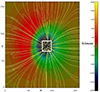Fig. 6. Artificial line of sight magnetogram of dimensions 160×160 used as the lower base for the computational box for reconstructing the magnetic field. The white square of dimensions 20×20 gridpoints indicates a portion of the active region where fluctuations were analysed. The colour bar represents the magnetic field intensity in Gauss.

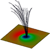Fig. 7. Reconstruction of 3D magnetic field by the COV method in the 20×20×100 flux tube.

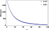Fig. 8. Average magnetic field for each layer in the x−y plane versus z for the COV and L&L models.

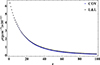Fig. 9. Behaviour of density for COV and L&L models.

Consequently, we constructed the matrices W and S, based on the magnetic field and density distributions inside the flux tube. Then, we extracted the oscillatory mode frequencies and expansion matrix according to the procedure described in Sect. 3.

The results for eigenfrequencies are shown in Table (2) and plotted in Fig. 10. The frequencies increase with mode number, k, and the corresponding periods range from 25.6 seconds for k = 1, to 3.8 seconds for k = 6. These oscillation periods may correspond to the short-period intensity oscillations observed in the solar corona (Cowsik et al. 1999; Rudawy et al. 2004; Rezaei et al. 2004; Nakariakov & Verwichte 2005; Gopalswamy et al. 2015; Mandal et al. 2016; Karampelas et al. 2019).

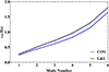Fig. 10. Illustration of the oscillatory mode frequencies versus mode number k = 1,2,…,6 and i=j = 2.

Using the results for the expansion matrix in Eq. (50), the x and y components of toroidal displacements that have opposite phases were calculated and are plotted in Fig. 11. As is clear in Fig. 11, the amplitude of these displacements decreases with increasing z.

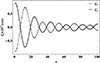Fig. 11. x and y components of displacements as a function of z.

We note that, in contrast to the unperturbed magnetic field, which has only a z-component, the perturbed magnetic field has only x and y components with opposite phases and both decrease with increasing z (see Fig. 12). Since the initial magnetic field is along the z-axis and is a function of z, the corresponding Lorentz force vanishes. However, after perturbation, the transverse motions induce the restoring Lorentz force, δF=δJ×B, which, just like δB, has only x and y components, as shown in Fig. 13. This force gives rise to the transverse Alfvén waves that propagate with the Alfvén velocity given by

$$v_A=\frac{|B|}{\sqrt{4\pi \rho }}·$$(60)

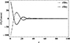Fig. 12. Illustration of the perturbed magnetic field components for i=j = 2 and k = 6.

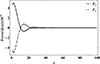Fig. 13. Lorentz force components versus z for COV and L&L models.

The variation of the Alfvén velocity in the flux tube as a function of z is shown in Fig. 14 for the COV and L&L methods, which are in agreement with Aschwanden et al. (1999).

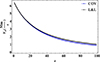Fig. 14. Alfvén velocity at different heights in COV and L&L models.

From an energy point of view, one deals with the following energies during the iterations and evolutions: (a) At the beginning of iteration, one has the potential magnetic field in the flux tube with the potential energy, E_pot, defined as

$$E_{\mathrm{pot}}=\int \mathrm{d}v\frac{B_{\mathrm{pot}}^2}{8\pi }·$$(61)

(b) At the end of the iteration, one has a non-linear force-free magnetic field, and the corresponding energy, E_nlff, is defined as

$$E_{\mathit{nlff}}=\int \mathrm{d}v\frac{B_{\mathit{nlff}}^2}{8\pi }·$$(62)

In Fig. 15, E_nlff/E_pot is plotted as a function of the iteration parameter that increases and approaches to an almost constant value 1.16 after 6000 iteration steps.

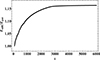Fig. 15. Variation of Enlff/Epot with iteration parameter.

(c) The energy due to the perturbation of the magnetic field, E_δB, is defined as

$$E_{\delta B}=\int \mathrm{d}\nu \frac{\delta B^2}{8\pi }·$$(63)

(d) The perturbation of the velocity field gives rise to kinetic energy, E_δv, given by

$$E_{\delta v}=\frac{1}{2}\int \mathrm{d}\nu \frac{1}{2}\rho (\delta v{)}^2.$$(64)

The values of the above energies for the COV and L&L models are given in Table 3. These values highlight the differences and similarities in energy distribution between the two methods.

The available restoring energy, E_rest, is given by the sum of magnetic free energy, E_free=E_nlff−E_pot, and perturbed energy, E_pert=E_δB+E_δv. Thus, E_rest=E_free+E_pert may contribute to the flaring and heating phenomena of the solar corona by some dissipation mechanism (Tadesse & Pevtsov 2013; Karami et al. 2002; Safari et al. 2006).

5. Conclusions

The magnetic field is the most important factor in generating the coronal phenomena. Due to the transparency of the coronal environment, direct observation of the magnetic field is still challenging. Therefore, semi-analytical or reconstruction methods may help to get insight into the coronal magnetic field. Here, we focus on reconstructing the magnetic field. Additionally, the study of coronal dynamics and fluctuations using a realistic magnetic field has not been thoroughly explored. In this work, we investigate the dynamics of the corona based on the reconstructed magnetic field according to the coronal conditions, which seems to be close to the real coronal magnetic field. One conventional method for determining the magnetic field is based on studies of solar corona fluctuations. Here, we employed a reverse method and used the reconstructed magnetic field to study the oscillations and wave propagation in the corona. The results for the oscillation periods are in agreement with observations (Bate et al. 2022; Nakariakov & Ofman 2001). The difference between the energies of non-linear force-free and potential magnetic fields has been considered as a factor in flare generation (Wiegelmann et al. 2017). In this study, by reconstructing the magnetic field and examining coronal dynamics, we also account for energy stored in MHD oscillations and mechanical waves, contributing to heating and flaring. In prior work (Fatholahzadeh et al. 2023), we proposed the COV method as an alternative for optimisation; this study validates that method. Usually, a uniform or semi-analytical magnetic field is used to examine solar corona fluctuations (Hasan & Sobouti 1987; Nasiri 1992). However, in this research, we reconstructed the magnetic field and its structure at every point within a box containing the coronal magnetic field. To do this, one can use either a real magnetogram based on photospheric data or an artificial magnetogram obtained by a semi-analytical method along with an optimisation procedure. As an optimisation technique, we used the vector Lagrangian multiplier method (COV) and placed the artificial magnetogram on the lower base of a 160×160×160 computational box. We then used Green's function method¹ to calculate the potential field based on appropriate boundary conditions, which then served as the input field in an iteration procedure. Further, we employed the vector Lagrangian multiplier technique (COV) to obtain the non-linear force-free magnetic field. The angle between the current density vector and the magnetic field was 7.647° for some 6000 iteration steps. Furthermore, the fractional increase in magnetic energy throughout the transition from the potential environment, which possesses the lowest energy value, toward the non-linear force-free state, that is,$\frac{E_{\mathit{nlff}}}{E_{\mathrm{pot}}}$, becomes 1.16. To validate our results we compared them with those of the semi-analytical L&L method, which yielded similar outcomes.

Next, we selected the active region located in the box and chose a portion of it, where the magnetic field could be assumed predominantly in the z-direction, as the lower base of a new computational box. We then induced a perturbation in this flux tube and investigated its oscillatory modes. Assuming the coronal conditions, we made the following assumptions: (a) The thermal pressure and gravitational forces were neglected, allowing us to disregard the p- and g-modes’ oscillations and focus only on the Lorentz force that generates the toroidal oscillations (t-mode). In the problem conditions of Cartesian coordinates and averaging each layer of the magnetic field and density, toroidal waves manifest themselves as transverse waves. (b) Due to the high magnetic Reynolds number, Re_m (which quantifies the ratio of magnetic advection to diffusion; see, e.g., Arfken & Weber 2012), in the solar corona, one deals with the frozen-in condition, allowing one to assume a linear relation with the mass density of the flux tube. Thus, the oscillatory mode frequencies and amplitudes of the transverse Alfvén waves were calculated using the Rayleigh-Ritz variational technique. The unperturbed current-free magnetic field is in the z direction only; however, the perturbed magnetic field coincides with the x,y plane and is no longer force free. The corresponding Lorentz force excites the transverse modes, giving rise to the transverse Alfvén waves.

In addition to magnetic free energy, which is the difference between non-linear and potential magnetic fields, there are kinetic and magnetic energies, which are caused by the perturbation and carried out by Alfvén waves. These energies, which have almost the same order of magnitude and may contribute to flaring and coronal heating by some dissipative mechanism, are calculated and given in Table (3).

Acknowledgments

The authors would like to thank the anonymous referee for their valuable comments and suggestions, which significantly improved the quality of this manuscript.

References

All Tables

All Figures

	Fig. 1. Artificial magnetogram of dimensions 160×160, obtained by the L&L method with parameters φ=π/8 and l = 0.5, with colour code in Gauss.
In the text

	Fig. 2. Behaviour of $\frac{L}{L_0}$ over 6000 iteration steps. L0 is the Lagrangian at the beginning of the iteration.
In the text

	Fig. 3. Angle (θ) between the magnetic field and electric current density vector, which reaches 7.647 with 6000 iteration steps.
In the text

	Fig. 4. Reconstruction of 3D magnetic fields for the box of dimensions 160 × 160 × 160 gridpoints.
In the text

	Fig. 5. Behaviour of λ versus iteration parameter. λmax is the maximum value of lambda in the last iteration.
In the text

	Fig. 6. Artificial line of sight magnetogram of dimensions 160×160 used as the lower base for the computational box for reconstructing the magnetic field. The white square of dimensions 20×20 gridpoints indicates a portion of the active region where fluctuations were analysed. The colour bar represents the magnetic field intensity in Gauss.
In the text

	Fig. 7. Reconstruction of 3D magnetic field by the COV method in the 20×20×100 flux tube.
In the text

	Fig. 8. Average magnetic field for each layer in the x−y plane versus z for the COV and L&L models.
In the text

	Fig. 9. Behaviour of density for COV and L&L models.
In the text

	Fig. 10. Illustration of the oscillatory mode frequencies versus mode number k = 1,2,…,6 and i=j = 2.
In the text

	Fig. 11. x and y components of displacements as a function of z.
In the text

	Fig. 12. Illustration of the perturbed magnetic field components for i=j = 2 and k = 6.
In the text

	Fig. 13. Lorentz force components versus z for COV and L&L models.
In the text

	Fig. 14. Alfvén velocity at different heights in COV and L&L models.
In the text

	Fig. 15. Variation of Enlff/Epot with iteration parameter.
In the text

References

- Altschuler, M. D., & Newkirk, G. 1969, Sol. Phys., 9, 131 [NASA ADS] [CrossRef] [Google Scholar]
- Altschuler, M. D., Levine, R. H., Stix, M., & Harvey, J. 1977, Sol. Phys., 51, 345 [NASA ADS] [CrossRef] [Google Scholar]
- Amari, T., Aly, J. J., Luciani, J. F., Boulmezaoud, T. Z., & Mikic, Z. 1997, Sol. Phys., 174, 129 [NASA ADS] [CrossRef] [Google Scholar]
- Amari, T., Boulmezaoud, T. Z., & Mikic, Z. 1999, A&A, 350, 1051 [NASA ADS] [Google Scholar]
- Arfken, G. B., & Weber, H. J. 2012, Mathematical Methods for Physicists (Academic Press) [Google Scholar]
- Aschwanden, M. 2005, Physics of the solar corona; An introduction with problems and solutions (Springer) [Google Scholar]
- Aschwanden, M. J. 2019, New Millennium Solar Physics (Springer Int. Publ.), 458 [Google Scholar]
- Aschwanden, M. J., Fletcher, L., Schrijver, C. J., & Alexander, D. 1999, ApJ, 520, 880 [Google Scholar]
- Bate, W., Jess, D. B., & Nakariakov, V. M. 2022, Astrophys. Res. Cent., 1, 1 [Google Scholar]
- Berghmans, D., & Clette, F. 1999, Sol. Phys., 186, 207 [Google Scholar]
- Čadež, V. 2005, Serb. Astron. J., 1, 171 [Google Scholar]
- Chen, P. F., et al. 2015, A&A, 581, A137 [NASA ADS] [CrossRef] [EDP Sciences] [Google Scholar]
- Chintzoglou, G., & Zhang, J. 2013, ApJ, 764, L3 [Google Scholar]
- Cowsik, R., Singh, J., Saxena, A., & Raveendran, A. 1999, Sol. Phys., 188, 89 [NASA ADS] [CrossRef] [Google Scholar]
- De Moortel, I., Walsh, R., & Ireland, J. 2000, A&A, 355, L23 [Google Scholar]
- Edwin, P., & Roberts, B. 1983, Sol. Phys., 88, 179 [Google Scholar]
- Edwin, P., & Roberts, B. 1988, A&A, 192, 343 [Google Scholar]
- Fatholahzadeh, S., Jafarpour, M. H., & Nasiri, S. 2023, A&A, 676, A120 [NASA ADS] [CrossRef] [EDP Sciences] [Google Scholar]
- Gary, G. A. 2001, Sol. Phys., 203, 71 [Google Scholar]
- Goossens, M., Hollweg, J. V., & Sakurai, T. 1992, Sol. Phys., 138, 233 [Google Scholar]
- Gopalswamy, N., Mäkelä, P., Akiyama, S., et al. 2015, ApJ, 806, 8 [Google Scholar]
- Grad, H., & Rubin, H. 1958, in Theoretical and experimental aspects of controlled nuclear fusion, Hydromagnetic equilibria and force-free fields, Second United Nations international conference on the peaceful uses of atomic energy, 31 [Google Scholar]
- Hasan, S. S., & Sobouti, Y. 1987, MNRAS, 228, 427 [Google Scholar]
- Jess, D. B., Reznikova, V. E., Ryans, R. S. I., et al. 2016, Nat. Phys., 12, 179 [NASA ADS] [CrossRef] [Google Scholar]
- Karami, K., Nasiri, S., & Sobouti, Y. 2002, A&A, 396, 993 [NASA ADS] [CrossRef] [EDP Sciences] [Google Scholar]
- Karampelas, K., Doorsselaere, T. V., Pascoe, D. J., & Guo, M. 2019, Front. Astron. Space Sci., 6, 1 [Google Scholar]
- Lin, H., Kuhn, J. R., & Coulter, R. 2004, ApJ, 613, L177 [Google Scholar]
- Low, B. C., & Lou, Y. Q. 1990, ApJ, 352, 343 [NASA ADS] [CrossRef] [Google Scholar]
- Mackay, D. H., Yeates, A. R., & Bocquet, F. -X. 2016, ApJ, 825, 131 [NASA ADS] [CrossRef] [Google Scholar]
- Mandal, S., Magyar, N., Yuan, D., Doorsselaere, T. V., & Banerjee, D. 2016, ApJ, 820, 13 [Google Scholar]
- Mikić, Z., Linker, J. A., Schnack, D. D., Lionello, R., & Tarditi, A. 1999, Phys. Plasmas, 6, 2217 [Google Scholar]
- Morton, R. J., et al. 2023, Rev. Mod. Plasma Phys., 7, 17 [NASA ADS] [CrossRef] [Google Scholar]
- Nakariakov, V. M., & Ofman, L. 2001, A&A, 372, L53 [NASA ADS] [CrossRef] [EDP Sciences] [Google Scholar]
- Nakariakov, V. M., & Verwichte, E. 2005, Living Rev. Sol. Phys., 2, 3 [Google Scholar]
- Nakariakov, V., Ofman, L., Deluca, E., Roberts, B., & Davila, J. 1999, Science, 285, 862 [Google Scholar]
- Nasiri, S. 1992, A&A, 261, 615 [NASA ADS] [Google Scholar]
- Nasiri, S., & Wiegelmann, T. 2019, J. Atmos. Sol.-Terr. Phys., 182, 181 [Google Scholar]
- Peter, H., Warnecke, J., Chitta, L. P., & Cameron, R. H. 2015, A&A, 584, A68 [NASA ADS] [CrossRef] [EDP Sciences] [Google Scholar]
- Petrie, G. J. D. 2024, J. Space Weather Space Clim., 14, 5 [Google Scholar]
- Petrova, E., Magyar, N., Doorsselaere, T. V., & Berghmans, D. 2023, ApJ, 1, 1 [Google Scholar]
- Priest, E. 2014, Magnetohydrodynamics of the Sun (Cambridge University Press) [Google Scholar]
- Rezaei, R., Singh, J., Cowsik, R., Sirinivasan, R., & Saxena, A. K. 2004, Iran. J. Phys. Res., 5, 6 [Google Scholar]
- Roberts, B., Edwin, P., & Benz, A. 1984, ApJ, 279, 857 [Google Scholar]
- Rudawy, P., Phillips, K. J. H., Gallagher, P. T., et al. 2004, A&A, 416, 1179 [NASA ADS] [CrossRef] [EDP Sciences] [Google Scholar]
- Ruderman, M. S., Verth, G., & Erdélyi, R. 2008, ApJ, 686, 694 [Google Scholar]
- Safari, H., Nasiri, S., Karami, K., & Sobouti, Y. 2006, A&A, 448, 375 [NASA ADS] [CrossRef] [EDP Sciences] [Google Scholar]
- Schrijver, C. J., De Rosa, M. L., Metcalf, T. R., et al. 2006, Sol. Phys., 235, 161 [NASA ADS] [CrossRef] [Google Scholar]
- Skirvin, S. J., Gao, Y., & Doorsselaere, T. V. 2023, ApJ, 1, 1 [Google Scholar]
- Sobouti, Y. 1977, A&A, 55, 327 [Google Scholar]
- Sobouti, Y. 1981, A&A, 100, 319 [NASA ADS] [Google Scholar]
- Sun, X., Hoeksema, J. T., Liu, Y., et al. 2012, ApJ, 748, 77 [Google Scholar]
- Tadesse, T., & Pevtsov, A. A. 2013, Sol. Phys., submitted [arXiv:1310.5790] [Google Scholar]
- Van Doorsselaere, T., Nakariakov, V. M., & Verwichte, E. 2008, ApJ, 676, L73 [Google Scholar]
- Verth, G., & Erdélyi, R. 2008, A&A, 486, 1015 [NASA ADS] [CrossRef] [EDP Sciences] [Google Scholar]
- Verwichte, E., Nakariakov, V., Ofman, L., & Deluca, E. 2004, Sol. Phys., 229, 187 [Google Scholar]
- Wang, T., & Solanki, S. 2004, A&A, 421, L33 [NASA ADS] [CrossRef] [EDP Sciences] [Google Scholar]
- Wang, T., Solanki, S., Innes, D., Curdt, W., & Marsch, E. 2003, A&A, 402, L17 [NASA ADS] [CrossRef] [EDP Sciences] [Google Scholar]
- Wheatland, M., Sturrock, P., & Roumeliotis, G. 2000, ApJ, 540, 1150 [Google Scholar]
- Wiegelmann, T. 2004, Sol. Phys., 219, 87 [NASA ADS] [CrossRef] [Google Scholar]
- Wiegelmann, T., Lagg, A., Solanki, S., Inhester, B., & Woch, J. 2005a, in Chromospheric and Coronal Magnetic Fields, eds. D. E. Innes, A. Lagg, & S. A. Solanki, ESA SP, 596, 7.1 [Google Scholar]
- Wiegelmann, T., Inhester, B., Lagg, A., & Solanki, S. K. 2005b, Sol. Phys., 228, 67 [NASA ADS] [CrossRef] [Google Scholar]
- Wiegelmann, T., Inhester, B., & Sakurai, T. 2006, Sol. Phys., 233, 215 [Google Scholar]
- Wiegelmann, T., Thalmann, J. K., Inhester, B., et al. 2012, Sol. Phys., 281, 37 [NASA ADS] [Google Scholar]
- Wiegelmann, T., Thalmann, J. K., & Solanki, S. K. 2014, A&A Rev., 22, 78 [Google Scholar]
- Wiegelmann, T., Petrie, G. J., & Riley, P. 2017, Space Sci. Rev., 210, 249 [CrossRef] [Google Scholar]
- Yang, Z., Bethge, C., Tian, H., et al. 2020a, Science, 369, 694 [Google Scholar]
- Yang, Z., Tian, H., Tomczyk, S., et al. 2020b, Sci. China Technol. Sci., 63, 2357 [CrossRef] [Google Scholar]