| Issue |
A&A
Volume 694, February 2025
|
|
|---|---|---|
| Article Number | A209 | |
| Number of page(s) | 9 | |
| Section | Planets, planetary systems, and small bodies | |
| DOI | https://doi.org/10.1051/0004-6361/202451693 | |
| Published online | 14 February 2025 | |
Background exoplanet candidates in the original Kepler field
1
Konkoly Observatory, HUN-REN Research Centre for Astronomy and Earth Sciences, MTA Centre of Excellence,
1121
Budapest,
Konkoly Thege Miklós út 15-17,
Hungary
2
Eötvös Loránd University, Institute of Physics and Astronomy,
1117
Budapest,
Pázmány Péter sétány 1/a,
Hungary
★ Corresponding author; john.bienias@csfk.org
Received:
29
July
2024
Accepted:
1
January
2025
Context. During the primary Kepler mission, between 2009 and 2013, about 150 000 pre-selected targets were observed with a 29.42 minute-long cadence. However, a survey of background stars that fall within the field of view of the downloaded apertures of the primary targets has revealed a number of interesting objects. In previous papers we have presented surveys of short-period eclipsing binaries and RR Lyrae stars.
Aims. The current survey of the Kepler background is concentrated on identifying longer-period eclipsing binaries and pulsating stars. These will be the subject of later papers. In the course of this survey, in addition to eclipsing binaries and pulsating stars, seven exoplanet candidates have been uncovered and in this paper we report on these candidates.
Methods. We used Lomb-Scargle, light curve transit search, and phase dispersion minimisation methods to reveal pixels that show significant periodicities, resulting in the identification of the seven exoplanet candidates. We prepared the light curves for analysis using Pytransit software and cross-matched the pixel coordinates with Gaia and other catalogues to identify the sources.
Results. We identify seven hot Jupiter exoplanet candidates with planet radii ranging from 0.8878 to 1.5174 RJup and periods ranging from 2.5089 to 4.7918 days.
Key words: planets and satellites: detection
© The Authors 2025
 Open Access article, published by EDP Sciences, under the terms of the Creative Commons Attribution License (https://creativecommons.org/licenses/by/4.0), which permits unrestricted use, distribution, and reproduction in any medium, provided the original work is properly cited.
This article is published in open access under the Subscribe to Open model. Subscribe to A&A to support open access publication.
1 Introduction
Since the first discovery of an exoplanet around 51 Peg (Mayor et al. 1995) and of the first transiting exoplanet in 1999 (Charbonneau et al. 2000; Henry et al. 2000), over 5600 exoplanets have been discovered. In the following decades, surveys such as the Optical Gravitational Lensing Experiment (OGLE) (Udalski et al. 1997), Convection, Rotation and planetary Transits (CoRoT) (Auvergne et al. 2009), Kepler (Borucki et al. 2010), and the ongoing Transiting Exoplanet Survey Satellite (TESS) (Ricker et al. 2015) have contributed to this dramatic rise in the number of known exoplanets.
The study of exoplanets is important for understanding how planetary systems form and evolve and for understanding whether and where life might exist elsewhere in the Universe. In addition, they give clues to how our own Solar System was formed.
In 2009, the Kepler photometric space telescope was launched into an Earth-trailing heliocentric orbit and was designed to detect exoplanets (and Earth-analogues in particular) by observing around 150000 target stars in a fixed 105 square degree area of the sky in the Cygnus, Lyra, and Draco constellations. A 4″ pixel size was used to provide a large full-well capacity and enable the high signal-to-noise ratio needed to detect Earth-sized planets. The observations were made with a 29.42 minute-long cadence over a period of 17 quarters from 2009 to 2013, at which time a second reaction control wheel failed and this part of the mission was terminated. For telemetry bandwidth reasons, only pixels of the target stars and their immediate surroundings were downloaded, and analysis of these images has focused on the pixels within the optimal apertures of the target stars. However, a pixel-by-pixel analysis of these images reveals a variety of interesting objects in the background.
In previous papers, we described detections of eclipsing binary stars (Bienias et al. 2021 and Forró & Szabó 2020) and RR Lyrae stars (Forró et al. 2022). The current survey was carried out with the primary objective of identifying longer-period eclipsing binary stars and pulsating stars, with periods up to approximately 90 days, and these will be the subjects of future papers. However, in the course of this survey, seven exoplanet candidates were identified and these are the subject of this paper.
In Sect. 2 we discuss data processing, including light curve processing and search methods, candidate selection, and the identification of host stars. In Sect. 3 we discuss the analysis of the candidates, including transit modelling, vetting, transit timing variation (TTV), stellar and planetary parameters, comparisons with known exoplanets, and selection biases. In Sect. 4 we briefly discuss our findings, and in Sect. 5 we give a summary of our work.
We note that in this paper the candidates are referred to by the Gaia EDR3 catalogue reference of the host star, followed by the Kepler Input Catalog (KIC) reference of the aperture in which they were found in brackets; for example, ‘Gaia DR3 2128959007378441472 (KIC 4459924)’.
2 Processing of Kepler data
2.1 Detrending procedure
The Kepler observations were made quasi-continuously over a 4-year period. However, the data are provided in discrete quarterly sets due to the 90-degree rolls required to maintain the correct orientation of the solar panels. Our initial search was restricted to the quarter 4 (Q4) observations, since this was the first relatively quiet quarter. All the individual pixels belonging to long-cadence Q4 KIC target apertures were used in the search.
The light curves were extracted for each individual pixel for each main target (denoted by KIC numbers) and detrended. This is a necessary precursor to generating the periodograms, as the drift in the light curves generates spurious frequencies in the area of interest. Searching individual pixels allows targets not located on a KIC aperture to be identified, as long as their Point Spread Functions (PSFs) overlap the aperture.
The quarterly light curves are subject to discontinuities and so each light curve was split into segments that could be detrended separately. Each segment was then detrended and normalised by fitting, and dividing by, a quadratic (one quadratic per segment) and the individual segments were then re-combined into a single light curve. A quadratic fit was used as some of the segments are relatively short and use of a higher order polynomial would likely remove any low frequency cyclic variation in such segments.
2.2 Search procedure
After detrending, a low-resolution Lomb-Scargle (Lomb 1976 and Scargle 1982) algorithm with a frequency interval of ≈0.01 cycles/day was employed to generate a periodogram for each pixel light curve. The resulting periodograms were searched for individual pixels showing a significant dominant frequency of less than four cycles/day (equivalent to a period of 6 hours for an exoplanet). ‘Significant’ means the amplitude is greater than four times the local background, that is
 (1)
(1)
where ad is the dominant frequency amplitude, aave is the average amplitude of the frequencies within ±0.5 c/d of the dominant frequency, and drms is the RMS deviation from aave of the frequencies within ±0.5 c/d of the dominant frequency. In many cases the dominant frequency was less than 0.5 cycles/day, and in these cases the background was measured between 0 and 1 cycle/day.
Even with detrending, the level of noise in the periodogram below approximately 0.13 cycles/day means that the effective upper period limit to the periodogram search is approximately 8 days for an exoplanet (16 days for an eclipsing binary). For this reason, we used a second routine to search the light curves and look for significant dips in the flux. As an experiment, we developed a simple search routine rather than using the more usual box least squares (BLS) approach. Testing showed this to be as sensitive as BLS analysis.
In this case, ‘a significant dip’ means an observation where the difference between the flux level and the average flux level is more than 3.5 times the RMS deviation of the observations, that is
 (2)
(2)
where fd is the flux of a single observation, fave is the average flux across the detrended light curve, and frms is the RMS deviation from fave of the flux across the light curve. A minimum of three such dips were required to select the light curve as a candidate. No requirement was made for the dips to be equally spaced, but subsequently, light curves and periodograms for all the candidates, found by either method, were visually inspected and false positives were discarded. We note that all of the exoplanet candidates in this paper were found with this second search method.
Checks were made for known objects, false positives (arising from bleeding, ghosting, or crosstalk), rotational variables, and duplicates (where a candidate PSF is detected in two KIC apertures) and these light curves were discarded. The individual pixel light curves for each remaining candidate were merged and detrended using the procedure described above.
For each candidate, a search was carried out on the relevant Q2–Q16 pixel light curves to identify the pixels that fold at the same frequency as the identified candidates. Between one and four pixels were found for each candidate for each quarter (though in some quarters no pixels were found or there were no data for the KIC aperture in question). Quarters 0, 1, and 17 were discarded as they are truncated and give rise to a disproportionate number of frequencies that differ significantly from those obtained from quarters 2 to 16. The resulting pixel light curves were then merged, detrended, and normalised to provide a set of quarterly light curves. These were then merged into a single Q2–Q16 light curve.
2.3 Exoplanet candidate selection
Initial candidate selection was based on the Q4 individual pixel light curves only. Light curves were classified as possible exoplanets if they met a number of criteria:
The light curve must have the correct morphology, that is, the continuum flux of the phase-folded light curve must be constant between transits.
The transit depth must be less than 2.5%.
There must be no apparent secondary eclipse.
The host star must be unambiguously identifiable (the source identification process is described in Sect. 2.7).
The Gaia catalogue entry for the host star must provide sufficient data to allow the radius of the star (and thus the exoplanet candidate radius and orbital radius) to be estimated.
Finally, after the quarterly light curves were combined into a single Q2–Q16 light curve, only those candidates were retained that had the typical planetary U-shaped transits. An example of a qualifying folded light curve is given in Fig. 1, which shows the Q4 light curve found in the background of the KIC 4459924 aperture and the folded Q2–Q16 light curve that shows the typical U-shaped exoplanet transit. Vetting of the selected candidates is described in Sect. 3.2.
2.4 Light curve de-blending
The candidate host stars all lie between approximately 5″ and 23″ from the (generally brighter) Kepler main targets, and are thus subject to light contamination from these same main targets. The effect of such contamination is to reduce the apparent fractional transit depths and thus the apparent radii of the candidate exoplanets.
PSFmachine is a software package specifically designed to de-blend Kepler light curves (Hedges & Martínez-Palomera 2023), and we employed it to generate de-blended light curves for each candidate and each quarter. Unfortunately, a number of issues arose, including a failure to produce some light curves, a lack of reproducibility in the generated light curves, and a lack of consistency across quarters, with quarterly light curves having quite wide variations in flux and transit depth. We speculate that this is due to the candidates mostly being located adjacent to, rather than on, their respective KIC apertures and the generally weak flux levels of the light curves. In one extreme case, Gaia DR3 2085335681690420608 (KIC 9674230), PSFmachine was unable to generate any light curves at all, possibly because of a weak light curve: only one pixel in each quarter exhibits a usable signal.
However, where PSFmachine was able to generate light curves, it enabled verification of the source stars. One candidate was eliminated as PSFmachine was able to show that the incorrect source star had been selected.
Instead of using PSFmachine, the candidate light curves were obtained by selecting and merging the pixel light curves that exhibited the best signals, that is, those with the deepest transit depths, and discarding those with lower transit depths, thus effectively minimising the light contamination from the main target. The residual main target contamination was then estimated for each quarterly light curve by plotting the distribution of the main target flux as a function of distance from the main target sky location. To a reasonable approximation, the main target flux decreases logarithmically with distance from the main target location. Figure 2 shows a typical example of this for the KIC 4459924 Q14 aperture. The estimated contamination obtained via this method was subtracted from the quarterly light curves for each candidate.
In some instances, particularly if the main target comprises only two or three pixels, this approach produces unrealistic results. In these cases, the contamination was taken from the corresponding quarters (that is, quarter numbers that differ by 4, 8, or 12 from the quarter in question), or, if this was not possible, the quarterly light curve was discarded. The contamination flux is significant, ranging from 10 to 40% of the total candidate flux.
Two of the candidate light curves, Gaia DR3 2100325529865507712 (KIC 4543171) and Gaia DR3 2079369937757906688 (KIC 9040849), have also been published by Martínez-Palomera et al. (2023), and we used these as a means of verifying the light curves we obtained. The results are shown in Sect. 3.1.
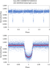 |
Fig. 1 (Top) Q4 light curve of the candidate found in the background of the KIC 4459924 aperture (before calculation of the zero epoch, BJD0), phase-folded as though it were an eclipsing binary. This meets the first three qualifying criteria for an exoplanet candidate. (Bottom) Phase-folded Q2–Q16 light curve of the candidate showing the U shape typical of a planetary transit. Blue dots are individual observations, and red circles are the phase bin mean fluxes. |
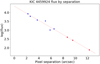 |
Fig. 2 Quarter 14 main-target average flux per pixel as a function of the separation (distance) of the pixel centre location from the main target location in arcsec (blue circles). The red line is the fit to log(flux), and the red circles indicate the extrapolation of the fitted line to the locations of the exoplanet candidate pixels. |
2.5 Determination of orbital periods
An initial estimate of the period was made by the light curve search routine, using the intervals between successive transits. This was not always accurate due to spurious dips in the flux. The smallest period value was selected to allow for missing transits. The estimates obtained were progressively improved, using the method we previously employed for eclipsing binary stars (Bienias et al. 2021) as follows:
-
For each quarterly light curve, a phase dispersion minimisation (PDM) algorithm was employed to search for the frequency (in a range of ±0.01 cycles/day around the initially obtained frequency), which yields the minimum dispersion (scatter) for the phase-folded light curve, that is, the minimum value of
 (3)
(3)where n = 30 is the number of phase bins, Oij is the jth observed flux value for the ith bin, and Ei is the average flux value for the ith bin. The average frequency thus obtained was used as the starting point for the following step.
The same PDM algorithm was employed, but with 500 phase bins and using the Q2–Q16 combined light curve to search for the best frequency in a range of ±0.01 cycles/day around the starting frequency. A fine adjustment was then made to the resulting frequency by fitting a parabola to the dispersion curve close to the minimum value. Figure 3 shows an example of a dispersion variation by frequency. The top panel shows a typical dispersion curve with a clearly defined minimum. The fit to the fine dispersion curve is shown in the bottom panel.
A further small adjustment was made to the period obtained using the TTV measurements described in Sect. 3.3.
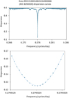 |
Fig. 3 (Top) Variation in PDM dispersion with frequency for the candidate in the background of the KIC 8293539 aperture. (Bottom) Dispersion points around the minimum, fitted with a parabola that gives a frequency = 0.2760227 cycles/day (period = 3.6228904 days). |
2.6 Determination of zero epoch
The phase-folded and binned light curves were used to determine the zero epoch of the exoplanet candidates. A quadratic was fitted to the transit, and the lowest point of this was assigned a phase value of zero. The last date before the start of the light curve that corresponded to this phase was assigned to the zero epoch, BJD0. However, we see from Fig. 4 that the transit shape does not lend itself well to a parabolic fit, and this initial value of BJD0 had to be corrected. This was done using the transit modelling described in Sect. 3.1 with a further correction obtained from the TTV analysis described in Sect. 3.3. These values are shown in Table A.4.
2.7 identification of host stars
The potential host stars for the exoplanet candidates were found from the right ascension (RA) and declination (Dec) of the main pixel, that is, the brightest pixel from the matching set. Candidates for the host stars are those at, or close to, the main pixel coordinates. In the majority of cases, the pixels found lie on the edge of the KIC aperture mask and the centre of the candidate PSF lies outside the mask. As a result, in some cases, there were several possible host stars for a single exoplanet candidate. These were discarded since it is not possible to reliably estimate the candidate planetary parameters.
An example is shown in Figs. 5 and 6. Figure 5 shows the pixel-by-pixel aperture mask for KIC 8175131. The RA and Dec. for the main pixel (row 695, column 305) were obtained using Astropy, and we searched the Gaia catalogue for all stars within 12″ (three pixels) of this location. These were then checked with Aladin to find the actual source. Figure 6, obtained from Aladin, shows the area of sky around this location, with the main pixel location, KIC 8175131 and the host star (Gaia DR3 2078315162505745920) marked. The identified Gaia catalogue references for the candidates are listed in Table A.1 together with their RA and Dec. and any alias identifiers.
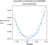 |
Fig. 4 Parabolic fit to a phase-folded and binned transit light curve used to calculate the initial value of BJD0 for the candidate. |
3 Candidate analysis
3.1 Transit modelling
Modelling of the exoplanet candidate light curves was performed using the PyTransit software package (Parviainen 2015). The software incorporates log posterior functions for transit modelling and parameter estimation. These store the observations and model priors to create a basis for Bayesian parameter estimation from transit light curves. They also contain methods for posterior optimisation and Markov chain Monte Carlo sampling.
PyTransit implements the quadratic limb darkening model of Mandel & Agol (2002) and Agol et al. (2020), so that, in general terms,
 (4)
(4)
where F is the observed fractional flux, I* is the stellar flux, Ī(k, ɡ) is the average limb-darkening-corrected flux covered by the planet, and A(k, ɡ) is the planet-star intersection area. The values Ī and A are expressed as functions of the planet-star radius ratio, k, and the grazing factor, ɡ, which is equal to b/(1 + k), where b is the impact parameter.
The principal parameters calculated by the model are (using the PyTransit notation):
b: the impact parameter, that is, the projected height of the transit above the stellar midline as a fraction of the stellar radius,
k: the ratio of the planet radius to the stellar radius,
u and v: the quadratic model limb-darkening coefficients,
a: the ratio of the orbital radius to the stellar radius,
i: the orbital inclination,
t14: the total duration of the transit,
t23: the duration of the complete transit,
e: the orbital eccentricity,
w: the argument of periastron.
The model was executed using the phase-folded individual observations of the normalised light curve, that is, with the orbital period set to 1.0 days. Given the probabilistic nature of the modelling, the model was executed twice for each candidate, with the same light curve data, to ensure that consistent results were obtained; that is, the differences in the transit parameters between executions were much smaller than the standard deviations of the parameters. In the worst case, the ratio of the difference between the values obtained from the two runs to the standard deviation value was 0.1142. This was for the value of k, for Gaia DR3 2100980735718445312 (KIC 4459924).
The results (that is, the average values of the two runs for each candidate) are shown in Table A.2. We note that, in all cases, the orbital eccentricity was negligibly small (of the order of 10−10) and is assumed to be zero. Thus e and w have been omitted from the table. It is noticeable that the sum of the impact parameter (b) and the planet-star radius ratio (k) is less than one in all cases, indicating that the transits are all full and there are no grazing transits.
In Appendix B we show the light curves obtained from the model. Each shows the individual observations and the model light curve overlaid with the phase-bin mean fluxes. The light curves all show the characteristic shape of a full, rather than grazing, transit, lending support to the calculated planetary radii.
In addition to the planetary and orbital parameters, the model identifies discrepancies between the zero phase point in the observations and the fitted model, and these discrepancies provide a correction to the value of BJD0. These corrections, and subsequent corrections identified by TTV analysis, are shown in Table A.4.
Two of the candidate light curves, Gaia DR3 2100325529865507712 (KIC 4543171) and Gaia DR3 2079369937757906688 (KIC 9040849), have also been published by Martínez-Palomera et al. (2023), and we modelled these with Pytransit as a means of assessing the reasonability of our light curves. The comparison of the principal Pytransit parameters (i, k and a) is shown in Table A.3. These are in reasonable agreement and lend confidence to our candidate light curves.
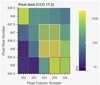 |
Fig. 5 KIC 8175131 aperture mask with the exoplanet candidate pixels outlined in red. The four bright pixels used in the Kepler pipeline to extract the main target light curve are outlined in white. (source: Lightkurve). |
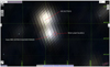 |
Fig. 6 Aladin sky map showing the area around KIC 8175131. The main pixel locations for the exoplanet candidate and the host star (Gaia DR3 2078315162505745920) are marked. The field of view is 34.31″ across. |
3.2 Candidate vetting
3.2.1 Odd-even transit comparison
The odd-numbered and even-numbered transits for each candidate were subjected to separate PyTransit fits to ensure that the transit depths were the same in each case. A significant difference would indicate that the candidate is an eclipsing binary rather than an exoplanet. The results are shown in Table A.7. For each candidate we show the difference between the odd-and even-numbered transit depths and the full light curve transit depth expressed as a fraction of the 1σ uncertainty in the full light curve transit depth. In all cases, the transit depth differences fall within the 1σ range.
The odd- and even-numbered Pytransit model fits are also shown graphically in Appendix C. For each candidate, we show the model fit to the odd- and even-numbered transits, the minimum flux obtained from the full light curve, and the estimated 1σ error in the minimum flux.
3.2.2 Centroid vetting
Centroid vetting is the means by which a candidate star is verified as being the true source of an interesting signal, rather than being contaminated by a background star. A significant centroid offset is evidence that the selected candidate is a false positive.
For this purpose, we employed the Vetting python package (Hedges 2021), which was constructed specifically for Kepler light curves and carries out in-transit and out-of-transit tests to ensure that a light curve signal is centred on the selected candidate. The test was run for each candidate and quarter, and generally confirmed the candidate host stars. However, there are limitations that prevent Vetting from analysing some light curves:
The pixel mask for the candidate cannot be in a 1xn format. Thus a minimum of three pixels, which must not be in a single row or column, is required for the test to work. For a number of candidates and quarters, only one or two pixels are available.
The KIC aperture must not be too crowded.
In cases where centroid testing could be carried out, that is, where there were sufficient pixels and the KIC aperture was not too crowded, the candidates were mostly confirmed to be the source. However, there were exceptions:
Gaia DR3 2078315162505745920 (KIC 8175131): offsets were detected in Q8 and Q16, but not in Q4 and Q12. The same pixel mask was used in each case. There were insufficient pixels in the other quarters.
Gaia DR3 2126910621514995968 (KIC 8293539): offsets were detected in Q3 and Q7, but not in Q4, Q8, Q12, and Q16. This is illustrated in Fig. 7, which shows the Q3 and Q4 Vetting output for this candidate. There were insufficient pixels in other quarters.
Gaia DR3 2079369937757906688 (KIC 9040849): the KIC aperture was too crowded. No testing could be carried out.
Gaia DR3 2085335681690420608 (KIC 9674230): there was only one relevant pixel in each of the quarters. No testing could be carried out.
3.3 Transit timing variation (TTV)
In a multi-planet system the gravitational effects of the planets on each other can perturb the timings of their transits, and by measuring these timing variations in one planet, it may be possible to infer the existence of other planets. On this subject, we refer the reader to Ballard et al. (2011), for example. Typically, a cyclic variation in the transit timing would indicate the presence of another planet. We carried out such a TTV analysis on the candidate light curves and no such variations were observed; we have therefore found no evidence for more planets in any of the systems examined.
However, all of the TTV analyses showed a small linear trend and small non-zero values for the average variation. These are assumed to arise from errors in the orbital period and BJD0. Corrections were made to the period using the linear trend gradient and to BJD0 using the average timing variation. After re-running the TTV with the corrected values, these discrepancies were mostly removed. Figure 8 shows a TTV chart before corrections were applied to BJD0 and the orbital period, and the trend is clear. The trend line has a gradient of −1.577E-06 and the average variation = −7.585E-05 (equivalent to a BJD0 correction of −2.475E-04 days). The results of the corrections are shown in Table A.4.
3.4 Host star parameters
The Gaia catalogue provides values of apparent magnitude, mG*, effective temperature, T* and gravity, log(ɡ*), of the candidate host stars. In addition, we have taken the photogeometric distance, d, to each star as calculated by Bailer-Jones et al. (2021).
Together, these allow estimations to be made of the stellar absolute magnitude, MG*, luminosity, L*, radius, R*, and mass, M*, using the standard equations:
 (5)
(5)
 (6)
(6)
 (7)
(7)
![${{{M_*}} \over {{M_ \odot }}} = {\left( {{{{R_*}} \over {{R_ \odot }}}} \right)^2} \cdot {10^{\left[ {\log \left( {{_*}} \right) - \log \left( {{_ \odot }} \right)} \right]}}.$](/articles/aa/full_html/2025/02/aa51693-24/aa51693-24-eq8.png) (8)
(8)
With these, estimates of the absolute (rather than relative) values of the exoplanet-candidate planetary and orbital radii have been obtained. In addition, from the stellar mass together with the orbital period, PP, the orbital radius, aP, in AU can be estimated independently of the PyTransit model using the standard equation:
![${a_P} = {\left[ {{{\left( {{{{P_P}} \over {{P_ \oplus }}}} \right)}^2} \cdot \left( {{{{M_*}} \over {{M_ \odot }}}} \right)} \right]^{1/3}}.$](/articles/aa/full_html/2025/02/aa51693-24/aa51693-24-eq9.png) (9)
(9)
The stellar parameters derived are shown in Table A.5. The planetary radius estimates and both orbital radius estimates are included in Table A.6.
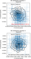 |
Fig. 7 Vetting output for Gaia DR3 2126910621514995968 (KIC 8293539) Q3 (top) where an offset was detected and Q4 (bottom) where no offset was detected. |
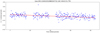 |
Fig. 8 Initial TTV analysis for Gaia DR3 2100325529865507712 (KIC 4543171) showing the observed − calculated (O - C) values of the transit times before the BJD0 and period corrections were applied. The gradient of the red trend line = −1.577E-06 and the average variation = −7.585E-05. We note that the time values are in orbital periods (= 3.2630113 days). |
3.5 Comparison with confirmed planets
The exoplanet candidates described in this work were compared with the confirmed exoplanets listed in the NASA Exoplanet Archive (NEA)1. Figure 9 shows the exoplanet radii plotted as a function of orbital radii. All the candidates lie within the clump of confirmed planets with radii between approximately 1 and 2 RJup and with orbital radii between 0.01 and 0.1 AU. Similarly, Figs. 10 and 11 show the exoplanet radii plotted as functions of the orbital period and transit depth, respectively.
There is no generally accepted definition of a hot Jupiter, but Fressin et al. (2013) define it as having 0.8 ≤ P ≤ 10.0 days and 6.0 R⊕ ≤ RP ≤ 22.0 R⊕, and Howard et al. (2012) define it as having P ≤ 10.0 days and 8.0 R⊕ ≤ RP ≤ 32.0 R⊕. If we accept these definitions, then the candidates are all hot Jupiters.
3.6 Selection bias
The exoplanet candidates described in this work all conform to the definition of a hot Jupiter. In this section we consider whether this narrow range may be due to selection bias.
3.6.1 Planet radius bias
The maximum radius limit for an exoplanet detection is determined by the arbitrary transit depth limit of 2.5% described in Sect. 2.3. This equates to a planet with a radius of approximately 1.6 RJup, assuming a solar-sized host star. However, this does not allow for correction for light contamination or for larger-sized host stars. Assuming a typical light contamination level of 20% and a maximum host star radius of 1.5 R⊙, then the largest detectable exoplanet will have a radius of approximately 2.6 RJup.
The minimum radius limit for exoplanet detection is determined principally by the quality of the individual pixel light curves: from Eq. (2) we see that the lower the level of scatter in the light curve, the shallower the transit depth that can be detected. The stars examined in this work are generally fainter than the main target stars: the host stars for the eight candidates have an average mG of 15.96, about two magnitudes dimmer than the average main target. Moreover, the host star locations mostly lie outside of the main target apertures, and only the edges of their PSFs are detected. As a result, the light curves are generally weak and noisy in comparison with the main targets, and the possibility of detecting small planets is remote.
A realistic test for the smallest detectable planet was made by using the individual Q4 pixel light curves from which the exoplanet candidates were originally identified. For each light curve, the transit depths were progressively reduced until the search routine described in Sect. 2.2 could no longer detect the transits. Figure 12 shows the results of this, with the minimum detectable fractional transit depth plotted as a function of the standard deviation, σ, of the normalised light curve (blue circles). The red line is the expected lower detection limit of 3.5σ. The minimum detection levels are mostly close to this line. The lowest detectable transit depth is 0.0025 for Gaia DR3 2100980735718445312 (KIC 4459924). The corresponding minimum and maximum planet sizes depend on the stellar radius, and Table 1 shows the minimum and maximum planet radii for a range of stellar radii from 0.1 to 1.5 R⊙. These are based on an upper limit of 0.025 fractional transit depth and a lower limit of 0.0025 fractional transit depth and include a correction for a typical light-contamination level of 20%.
A similar calculation was carried out using the full Q2–Q16 light curves. The minimum detectable fractional transit depth is 0.0018 for Gaia DR3 2100325529865507712 (KIC 4543171), resulting in slightly smaller minimum detectable planet sizes (shown in the right-hand column of Table 1). The results are also shown in Fig. 12 (orange triangles). We note that one candidate was not detected at all in the Q2–Q16 light curves: Gaia DR3 2085335681690420608 (KIC 9674230). This arises from the merging of the Q4 (and Q8, Q12, and Q16) light curves with the Q3, Q7, Q11, and Q15 light curves, which are of relatively poor quality, thus increasing the level of scatter in the Q2–Q16 light curve.
In principle then, Earth-sized planets orbiting small stars should be detectable. However, Fig. 13 shows the radii of the known exoplanets listed in the NEA database plotted as a function of their host star radii, along with the exoplanet candidates. Lines on the chart show the Q4 and the Q2 - Q16 minimum detectable planet radii given in Table 1. These clearly indicate that planets with a radius <0.5RJup are almost entirely outside the detectable range.
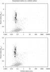 |
Fig. 9 Confirmed exoplanets in the NEA database with radii up to 2.5 RJup (open grey circles) and the seven exoplanet candidates identified in this work (black circles). The top panel shows the orbital radii calculated using the orbital period and stellar mass in Table A.5, i.e. Column “Orb. Rad.(1)” in Table A.6, and the bottom panel shows those calculated using the planet orbit-star radius ratio and the stellar radius in A.5, i.e. Column “Orb. Rad. (2)” in Table A.6. The error bars reflect the low and high values shown in the table. |
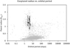 |
Fig. 10 Confirmed exoplanets in the NEA database with radii up to 2.5 RJup (open grey circles) and the seven exoplanet candidates identified in this work (black circles). The orbital periods are those shown in Table A.6. The error bars reflect the low and high values shown in the table. |
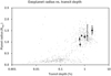 |
Fig. 11 Confirmed exoplanets in the NEA database with radii up to 2.5 RJup (open grey circles) and the seven exoplanet candidates identified in this work (black circles). The transit depths are taken from the minimum flux values derived from the Pytransit model for each candidate. The error bars reflect the 1σ uncertainty in the transit depth. |
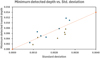 |
Fig. 12 Minimum detectable fractional transit depth for the exoplanet candidates as a function of the standard deviation, σ, of the normalised pixel light curves (blue circles) and the normalised Q2–Q16 light curves (orange triangles). The red line is the expected lower limit of 3.5σ. |
Minimum and maximum detectable planet radii.
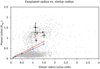 |
Fig. 13 Confirmed exoplanets on the NEA database with radii up to 2.5 RJup (open grey circles) and the seven exoplanet candidates identified in this work (black circles) plotted against their host star radii. The minimum detectable planet radii derived from the Q4 light curves (red circles and line) and from the Q2–Q16 light curves (blue circles and line) given in Table 1 are also shown. |
3.6.2 Orbital period bias
The search routine used requires a minimum of three transits to be detected within the Q4 light curves. Thus, in principle, all exoplanets with periods of up to 30 days should be detected (assuming a light curve of sufficiently good quality) and up to 45 days if the transits are fortuitously located within the light curve. Clearly, this has not happened, with the maximum detected period being 4.791774 days for Gaia DR3 2100980735718445312 (KIC 4459924). However, Fig. 10 shows that known Jupiter-sized planets are concentrated in the period range 1 ≤ P ≤ 10 days and comparatively few have longer periods. The chances of detecting one are low.
4 Results
The results of the PyTransit modelling are shown in Table A.2. These, combined with the stellar parameters shown in Table A.5 were used to calculate the planetary parameters shown in Table A.6. These clearly indicate that all the candidates are hot-Jupiter types, with planet radii ranging from 0.8878 to 1.5174 RJup and orbital radii ranging from 0.0437 to 0.0653 AU or 0.0293 - 0.0495 AU depending on which calculations are used.
The light curves, together with the fitted PyTransit models, are shown in Appendix B. The fits are good, with the phase-bin mean fluxes generally within one standard error of the model fit. The light curves all exhibit the characteristic shape of a full, rather than grazing, transit, thus supporting the planetary radii obtained from the Pytransit modelling.
Transit timing variation analysis was applied to the light curves, but no evidence was found of second planets. Comparison of the candidates with confirmed planets in the NEA database shows that the planetary parameters of the exoplanet candidates are all consistent with confirmed hot-Jupiter exoplanets. It should be noted that work by Santerne et al. (2012) suggests a false positive rate of approximately 35% for close-in Jupiter candidates, and it must be expected that only perhaps four or five of the candidates in this paper will eventually be confirmed.
5 Summary
We conducted a survey searching for pulsating stars and eclipsing binaries in the background pixels of the observed KIC targets in the original Kepler field in the period range up to ~90 days. In the course of this search, we found seven exoplanet candidates, which we have presented in this paper.
We prepared the light curves for each quarter and each candidate for further analysis, that is, we detrended and normalised the quarter light curves and then combined them to form ~3.5 yearlong datasets (excluding quarters 0,1, and 17). We cross-matched the pixel coordinates with the Gaia catalogue to identify the host star candidates.
We analysed the transit light curves using the PyTransit software package and determined the planetary parameters. Using the stellar data available from the Gaia catalogue, we estimated the candidate planet radii and orbital radii. All of the seven candidates are consistent with hot-Jupiter-type planets. The planetary parameters are also consistent with the known exoplanets listed in the NEA database.
We carried out candidate vetting, including odd-even transit modelling and centroid analysis, to strengthen the case for the candidates being exoplanets.We carried out TTV analysis to search for second planets in the systems, but no evidence for these was found. The candidate light curves taken together with the Pytransit models and the comparison with known exoplanets provide strong support for these candidates being exoplanets. The results of the survey for pulsating variables and long-period eclipsing binaries will be presented in subsequent papers.
Data availability
Appendix B: Pytransit model fits
Appendix C: PyTransit odd and even transit model fits
Acknowledgements
This paper includes data collected by the Kepler mission. Funding for the Kepler mission is provided by the NASA Science Mission directorate. This research was supported by the KKP-137523 ‘SeismoLab’ Élvonal grant and the SNN-147362 grant of the Hungarian Research, Development and Innovation Office (NKFIH). This work has made use of data from the European Space Agency (ESA) mission Gaia (https://www.cosmos.esa.int/gaia), processed by the Gaia Data Processing and Analysis Consortium (DPAC, https://www.cosmos.esa.int/web/gaia/dpac/consortium). Funding for the DPAC has been provided by national institutions, in particular the institutions participating in the Gaia Multilateral Agreement. This research has made use of the NASA Exoplanet Archive, which is operated by the California Institute of Technology, under contract with the National Aeronautics and Space Administration under the Exoplanet Exploration Program. We have also made use of the VizieR catalogue access tool, CDS, Strasbourg, France (DOI: 10.26093/cds/vizier). The original description of the VizieR service was published in A&AS 143, 23. The research was also carried out with the use of a number of other facilities which we gratefully acknowledge: PyTransit, a Python package for the analysis and modelling of transiting exoplanet light curves (Parviainen 2015). Lightkurve, a Python package for Kepler and TESS data analysis (Lightkurve Collaboration et al. 2018). The “Aladin sky atlas” developed at CDS, Strasbourg Observatory, France (Bonnarel et al. 2000). Astropy2, a community-developed core Python package for Astronomy (Astropy Collaboration 2013). PSFmachine, a Python package for deblending Kepler light curves (Hedges & Martínez-Palomera 2023). Vetting, a Python package for centroid testing of transits and eclipses (Hedges 2021).
References
- Agol, E., Luger, R., & Foreman-Mackey, D. 2020, AJ, 159, 123 [Google Scholar]
- Astropy Collaboration (Robitaille, T. P., et al.) 2013, A&A, 558, A33 [NASA ADS] [CrossRef] [EDP Sciences] [Google Scholar]
- Auvergne, M., Bodin, P., Boisnard, L., et al. 2009, A&A, 506, 411 [NASA ADS] [CrossRef] [EDP Sciences] [Google Scholar]
- Bailer-Jones, C. A. L., Rybizki, J., Fouesneau, M., Demleitner, M., & Andrae, R. 2021, AJ, 161, 147 [Google Scholar]
- Ballard, S., Fabrycky, D., Fressin, F., et al. 2011, ApJ, 743, 200 [NASA ADS] [CrossRef] [Google Scholar]
- Bienias, J., Bódi, A., Forró, A., Hajdu, T., & Szabó, R. 2021, ApJS, 256, 11 [CrossRef] [Google Scholar]
- Bonnarel, F., Fernique, P., Bienaymé, O., et al. 2000, A&AS, 143, 33 [NASA ADS] [CrossRef] [EDP Sciences] [Google Scholar]
- Borucki, W. J., Koch, D., Basri, G., et al. 2010, AAS Meeting Abstracts, 215, 101.01 [NASA ADS] [Google Scholar]
- Charbonneau, D., Brown, T. M., Latham, D. W., & Mayor, M. 2000, ApJ, 529, L45 [Google Scholar]
- Forró, A., & Szabó, R. 2020, Contrib. Astron. Observ. Skal. Pleso, 50, 405 [Google Scholar]
- Forró, A., Szabó, R., Bódi, A., & Császár, K. 2022, ApJS, 260, 20 [CrossRef] [Google Scholar]
- Fressin, F., Torres, G., Charbonneau, D., et al. 2013, ApJ, 766, 81 [NASA ADS] [CrossRef] [Google Scholar]
- Hedges, C. 2021, Res. Notes AAS, 5, 262 [NASA ADS] [CrossRef] [Google Scholar]
- Hedges, C., & Martínez-Palomera, J. 2023, Astrophysics Source Code Library [record ascl:2306.056] [Google Scholar]
- Henry, G. W., Marcy, G. W., Butler, R. P., & Vogt, S. S. 2000, ApJ, 529, L41 [Google Scholar]
- Howard, A. W., Marcy, G. W., Bryson, S. T., et al. 2012, ApJS, 201, 15 [Google Scholar]
- Lightkurve Collaboration, Cardoso, J. V. d. M., Hedges, C., et al. 2018, Astro physics Source Code Library [record ascl:1812.013] [Google Scholar]
- Lomb, N. R. 1976, Ap&SS, 39, 447 [Google Scholar]
- Mandel, K., & Agol, E. 2002, ApJ, 580, L171 [Google Scholar]
- Martínez-Palomera, J., Hedges, C., & Dotson, J. 2023, AJ, 166, 265 [CrossRef] [Google Scholar]
- Mayor, M., Queloz, D., Marcy, G., et al. 1995, IAU Circ., 6251, 1 [Google Scholar]
- Parviainen, H. 2015, MNRAS, 450, 3233 [Google Scholar]
- Ricker, G. R., Winn, J. N., Vanderspek, R., et al. 2015, J. Astron. Teles. Instrum. Syst., 1, 014003 [Google Scholar]
- Santerne, A., Díaz, R. F., Moutou, C., et al. 2012, A&A, 545, A76 [NASA ADS] [CrossRef] [EDP Sciences] [Google Scholar]
- Scargle, J. D. 1982, ApJ, 263, 835 [Google Scholar]
- Udalski, A., Kubiak, M., & Szymanski, M. 1997, Acta Astron., 47, 319 [NASA ADS] [Google Scholar]
All Tables
All Figures
|
Fig. 1 (Top) Q4 light curve of the candidate found in the background of the KIC 4459924 aperture (before calculation of the zero epoch, BJD0), phase-folded as though it were an eclipsing binary. This meets the first three qualifying criteria for an exoplanet candidate. (Bottom) Phase-folded Q2–Q16 light curve of the candidate showing the U shape typical of a planetary transit. Blue dots are individual observations, and red circles are the phase bin mean fluxes. |
| In the text | |
|
Fig. 2 Quarter 14 main-target average flux per pixel as a function of the separation (distance) of the pixel centre location from the main target location in arcsec (blue circles). The red line is the fit to log(flux), and the red circles indicate the extrapolation of the fitted line to the locations of the exoplanet candidate pixels. |
| In the text | |
|
Fig. 3 (Top) Variation in PDM dispersion with frequency for the candidate in the background of the KIC 8293539 aperture. (Bottom) Dispersion points around the minimum, fitted with a parabola that gives a frequency = 0.2760227 cycles/day (period = 3.6228904 days). |
| In the text | |
|
Fig. 4 Parabolic fit to a phase-folded and binned transit light curve used to calculate the initial value of BJD0 for the candidate. |
| In the text | |
|
Fig. 5 KIC 8175131 aperture mask with the exoplanet candidate pixels outlined in red. The four bright pixels used in the Kepler pipeline to extract the main target light curve are outlined in white. (source: Lightkurve). |
| In the text | |
|
Fig. 6 Aladin sky map showing the area around KIC 8175131. The main pixel locations for the exoplanet candidate and the host star (Gaia DR3 2078315162505745920) are marked. The field of view is 34.31″ across. |
| In the text | |
|
Fig. 7 Vetting output for Gaia DR3 2126910621514995968 (KIC 8293539) Q3 (top) where an offset was detected and Q4 (bottom) where no offset was detected. |
| In the text | |
|
Fig. 8 Initial TTV analysis for Gaia DR3 2100325529865507712 (KIC 4543171) showing the observed − calculated (O - C) values of the transit times before the BJD0 and period corrections were applied. The gradient of the red trend line = −1.577E-06 and the average variation = −7.585E-05. We note that the time values are in orbital periods (= 3.2630113 days). |
| In the text | |
|
Fig. 9 Confirmed exoplanets in the NEA database with radii up to 2.5 RJup (open grey circles) and the seven exoplanet candidates identified in this work (black circles). The top panel shows the orbital radii calculated using the orbital period and stellar mass in Table A.5, i.e. Column “Orb. Rad.(1)” in Table A.6, and the bottom panel shows those calculated using the planet orbit-star radius ratio and the stellar radius in A.5, i.e. Column “Orb. Rad. (2)” in Table A.6. The error bars reflect the low and high values shown in the table. |
| In the text | |
|
Fig. 10 Confirmed exoplanets in the NEA database with radii up to 2.5 RJup (open grey circles) and the seven exoplanet candidates identified in this work (black circles). The orbital periods are those shown in Table A.6. The error bars reflect the low and high values shown in the table. |
| In the text | |
|
Fig. 11 Confirmed exoplanets in the NEA database with radii up to 2.5 RJup (open grey circles) and the seven exoplanet candidates identified in this work (black circles). The transit depths are taken from the minimum flux values derived from the Pytransit model for each candidate. The error bars reflect the 1σ uncertainty in the transit depth. |
| In the text | |
|
Fig. 12 Minimum detectable fractional transit depth for the exoplanet candidates as a function of the standard deviation, σ, of the normalised pixel light curves (blue circles) and the normalised Q2–Q16 light curves (orange triangles). The red line is the expected lower limit of 3.5σ. |
| In the text | |
|
Fig. 13 Confirmed exoplanets on the NEA database with radii up to 2.5 RJup (open grey circles) and the seven exoplanet candidates identified in this work (black circles) plotted against their host star radii. The minimum detectable planet radii derived from the Q4 light curves (red circles and line) and from the Q2–Q16 light curves (blue circles and line) given in Table 1 are also shown. |
| In the text | |
Current usage metrics show cumulative count of Article Views (full-text article views including HTML views, PDF and ePub downloads, according to the available data) and Abstracts Views on Vision4Press platform.
Data correspond to usage on the plateform after 2015. The current usage metrics is available 48-96 hours after online publication and is updated daily on week days.
Initial download of the metrics may take a while.