| Issue |
A&A
Volume 691, November 2024
|
|
|---|---|---|
| Article Number | A223 | |
| Number of page(s) | 14 | |
| Section | Stellar structure and evolution | |
| DOI | https://doi.org/10.1051/0004-6361/202451247 | |
| Published online | 15 November 2024 | |
Advanced classification of hot subdwarf binaries using artificial intelligence techniques and Gaia DR3 data
1
Institute of Theoretical Physics and Astronomy, Vilnius University, Sauletekio av. 3, 10257 Vilnius, Lithuania
2
Centro de Astrobiología (CSIC-INTA), Camino Bajo del Castillo s/n, E-28692 Villanueva de la Cañada, Madrid, Spain
3
Applied Physics Department, Universidade de Vigo, Campus Lagoas-Marcosende, s/n, E-36310 Vigo, Spain
4
Centro de Investigación Mariña, Universidade de Vigo, GEOMA, Edificio Olimpia Valencia, Campus Lagoas-Marcosende, E-36310 Vigo, Spain
5
CIGUS CITIC – Department of Computer Science and Information Technologies, University of A Coruña, s/n, E-15071 A Coruña, Spain
6
CIGUS CITIC – Department of Nautical Sciences and Marine Engineering, University of A Coruña, Paseo de Ronda 51, E-15011 A Coruña, Spain
7
INAF – Osservatorio Astrofisico di Arcetri, Largo E. Fermi 5, 50125 Firenze, Italy
8
IES de Beade, Consellería de Educación e Ordenación Universitaria, Camino do Outeiro 10, E-36312 Vigo, Spain
9
Observatorio Astronómico Nacional (OAN), Alfonso XII 3, 28014 Madrid, Spain
⋆ Corresponding author; carlos.viscasillas@ff.vu.lt
Received:
25
June
2024
Accepted:
24
September
2024
Context. Hot subdwarf stars are compact blue evolved objects, burning helium in their cores surrounded by a tiny hydrogen envelope. In the Hertzsprung-Russell Diagram they are located by the blue end of the Horizontal Branch. Most models agree on a quite probable common envelope binary evolution scenario in the Red Giant phase. However, the current binarity rate for these objects is yet unsolved, but key, question in this field.
Aims. This study aims to develop a novel classification method for identifying hot subdwarf binaries within large datasets using Artificial Intelligence techniques and data from the third Gaia data release (GDR3). The results will be compared with those obtained previously using Virtual Observatory techniques on coincident samples.
Methods. The methods used for hot subdwarf binary classification include supervised and unsupervised machine learning techniques. Specifically, we have used Support Vector Machines (SVM) to classify 3084 hot subdwarf stars based on their colour-magnitude properties. Among these, 2815 objects have Gaia DR3 BP/RP spectra, which were classified using Self-Organizing Maps (SOM) and Convolutional Neural Networks (CNN). In order to ensure spectral quality, previously to SOM and CNN classification, our 2815 BP/RP set were pre-analysed with two different approaches: the cosine similarity technique and the Uniform Manifold Approximation and Projection (UMAP) technique. Additional analysis onto a golden sample of 88 well-defined objects, is also presented.
Results. The findings demonstrate a high agreement level (∼70–90%) with the classifications from the Virtual Observatory Sed Analyzer (VOSA) tool. This shows that the SVM, SOM, and CNN methods effectively classify sources with an accuracy comparable to human inspection or non-AI techniques. Notably, SVM in a radial basis function achieves 70.97% reproducibility for binary targets using photometry, and CNN reaches 84.94% for binary detection using spectroscopy. We also found that the single–binary differences are especially observable on the infrared flux in our Gaia DR3 BP/BR spectra, at wavelengths larger than ∼700 nm.
Conclusions. We find that all the methods used are in fairly good agreement and are particularly effective to discern between single and binary systems. The agreement is also consistent with the results previously obtained with VOSA. In global terms, considering all quality metrics, CNN is the method that provides the best accuracy. The methods also appear effective for detecting peculiarities in the spectra. While promising, challenges in dealing with uncertain compositions highlight the need for caution, suggesting further research is needed to refine techniques and enhance automated classification reliability, particularly for large-scale surveys.
Key words: methods: data analysis / techniques: spectroscopic / binaries: general / subdwarfs
© The Authors 2024
 Open Access article, published by EDP Sciences, under the terms of the Creative Commons Attribution License (https://creativecommons.org/licenses/by/4.0), which permits unrestricted use, distribution, and reproduction in any medium, provided the original work is properly cited.
This article is published in open access under the Subscribe to Open model. Subscribe to A&A to support open access publication.
1. Introduction
Hot subdwarf stars (hot sds) are a unique stellar class characterized by their luminosity, which is lower than that of main-sequence stars of the same spectral type. Kuiper (1939) and Humason & Zwicky (1947) were the first to detect and catalogue these stars, mainly classified into B (sdB) and O (sdO) types based on their atmospheric composition, with dominance of hydrogen (H) or helium (He), respectively (Drilling et al. 2013; Heber 2016).
Initially found at high galactic latitudes (e.g. Bixler et al. 1991; Moehler et al. 1990), more comprehensive searches (Luo et al. 2021; Culpan et al. 2022a; Dawson et al. 2024, and earlier) have shown that hot sds are found in all Galactic populations. In addition, hot sds in globular clusters have been studied in detail by Latour et al. (2023). On the other hand, asteroseismology has provided relevant insights into the internal structure and evolution of hot sds (see Lynas-Gray 2021, for a comprehensive review of hot subdwarf pulsations).
In the Hertzsprung-Russell Diagram, hot sds are located near the blue end of the horizontal branch (Greenstein & Sargent 1974), near the extended horizontal branch (EHB). With effective temperatures (Teff) exceeding ∼19 000 K, surface gravities (log g) in the range 4.5 ≤ log g ≤ 6.5 dex, masses around 0.5 M⊙, and a fraction of about 0.2 of the solar radius, they represent a late stage in stellar evolution, often formed when a red giant loses its outer hydrogen layers (Heber 2009, 2016). As a consequence, these stars lack the capacity for sustaining hydrogen shell burning, and they deviate from the conventional evolution path, do not ascend the asymptotic giant branch (AGB), and proceed directly onto the white dwarf (WD) cooling track (Heber 2016). This suggests enhancement of mass-loss efficiency (D’Cruz et al. 1996) or companion-driven mass transfer or coalescence. While Luo et al. (2024) conclude that the merging of double helium WD binaries cannot explain the formation of C-deficient He-rich hot sds, most models agree on a quite probable common envelope binary evolution scenario in the red giant (RG) phase (e.g. Kramer et al. 2020) because it is virtually impossible for a single RG to lose so much of its total mass on its own. The Pelisoli et al. (2020) results suggest that the involvement of binary interaction is always necessary for the formation of hot sdBs. Decades of observations seem to support this assumption (e.g.Dworetsky et al. 1977; Paczynski 1980; Ferguson et al. 1984; Kawka et al. 2015). For sdOs, less common and hotter than sdB stars, and which are believed to have a carbon and oxygen core surrounded by a helium-burning shell, some examples have been found as central stars of planetary nebulae (CSPNe), and even as binary systems (Aller et al. 2013, 2015).
As the main objectives of our work deal with the classification of composite hot subdwarf systems, it is worth indicating here some specific information on their formation and observational properties. In particular, composite subdwarf B (sdB) + main-sequence (MS) systems are critical for understanding the formation and observational properties of sdB stars. The different scenarios of sdB/Os and binary evolution are described in detail in Han et al. (2002) and Han et al. (2003). From population synthesis, a high binary fraction, up to 80%, was predicted by these authors. A more recent work on the helium-WD merger channel is Zhang & Jeffery (2012), among others.
Companions to hot sds are of varied nature, from A-type stars to degenerate objects. These systems typically form through binary interaction, as demonstrated in the works of Vos et al. (2012, 2013, 2017, 2018, 2020), which characterized long-period sdB binaries and their evolution histories. Pelisoli et al. (2020) further provided evidence that binary interaction is necessary for the formation of hot sds, highlighting the absence of wide sdB binaries that would suggest single-star formation scenarios. Additionally, recent findings by Lei et al. (2023) identified new long-period composite sdB binaries and emphasized the importance of binary interactions in their formation. Although inconclusive, the search for other types of companions to sdBs, including supermassive WDs (M > 1.0 M⊙), neutron stars, black holes, brown dwarfs, or even exoplanets, has been addressed over the years (e.g. Silvotti et al. 2007; Geier et al. 2011; Van Grootel et al. 2021; Thuillier et al. 2022; Schaffenroth et al. 2022, 2023).
From an observational perspective, composite hot sds have been extensively studied. Early works, for example those by Thejll et al. (1995) and Ulla & Thejll (1998), indicated that infrared flux excesses in the JHK bands were found to be mostly due to companion stars, typically of spectral types A-K, for about 44% of their sample. More recent studies (see e.g. Németh 2020), indicate that hot sds in close binaries have either low-mass K–M-type or WD companions; instead, when they are in wide binaries, they have more massive F–G-type companions. Typical binary periods of systems with low-mass MS companions are less than 30 days, with the detection of reflection effects at the shortest periods, especially for M-type companions. For the case of WD companions, ellipsoidal modulation and Doppler beaming have been found (Schaffenroth et al. 2023). On the other hand, wider hot sd binaries with orbital periods ranging from about 400 to 1500 days are where more massive F–G-type companions are found. In this case, double-lined composite spectra are often displayed and, in general, spectral decomposition techniques are required for proper analysis (Németh 2020). With regard to He content, radial velocity (RV) variability studies by Geier et al. (2022) reveal that He-poor hot sds display a high fraction of close binaries, while the He-rich hot sds RV variability values are almost not significant, probably indicating different evolutionary channels. Among other striking results found, these authors also indicate the possible existence of a new binary subpopulation of hot sds cooler than about 24 000 K, with long orbital periods, but late-type or compact companions. Further studies using space-based missions like the Transiting Exoplanet Survey Satellite (TESS, Ricker et al. 2015) have led to the discovery variable hot sds, both binary and pulsating, allowing the detailed analysis of their light curves, companion masses, and orbital parameters (Sahoo et al. 2020; Schaffenroth et al. 2023; Uzundag et al. 2024). These ongoing efforts are gradually improving our understanding of the binary nature and evolution of hot sds, and highlight the importance of refining classification methods.
The first catalogues including hot sds date back several decades (see e.g. Green et al. 1986; Kilkenny et al. 1988; Boyle et al. 1990; Kleinman et al. 2004; Mickaelian 2008). With the advent of the new spectroscopic surveys like the Massive Unseen Companions to Hot Faint Underluminous Stars project (MUCHFUSS, Geier et al. 2011; Schaffenroth et al. 2018) from the Sloan Digital Sky Survey (SDSS), or the Large Sky Area Multi-Object Fibre Spectroscopic Telescope (LAMOST, Cui et al. 2012; Luo et al. 2016), and space missions like Gaia (Geier et al. 2019; Culpan et al. 2022a), or combinations of them (Lei et al. 2018), the census of hot sds has increased significantly. This means that methodologies to analyse photometry and spectra must adapt to the large amounts of data provided (see e.g. Ambrosch et al. 2023).
Simultaneously with the exponential growth of data, initiatives such as the Virtual Observatory1 (VO) have proven to be very useful in facing new frontiers in the field of massive data analysis. Oreiro et al. (2011), using the VO methodology, designed a custom procedure to discover previously uncatalogued hot sds within blue object samples. This approach minimizes contamination on WDs, cataclysmic variables, and OB stars. Pérez-Fernández et al. (2016) further refined the methodology and successfully identified new hot sds with SDSS spectra. Next, Solano et al. (2022) presented a method for identifying binary systems involving hot sds, utilizing the VOSA Virtual Observatory tool (Bayo et al. 2008). The approach involves constructing the spectral energy distribution (SED) from ultraviolet to infrared wavelengths, identifying binaries through flux excess towards redder bands, and estimating physical parameters for both individual and composite hot sds based on the optimal fitting model (Rodrigo et al. 2020).
Recent studies have leveraged artificial intelligence (AI) techniques for the identification and classification of hot subdwarf stars, significantly enhancing automation and accuracy. Bu et al. (2019) employed a method combining convolutional neural networks (CNN) and support vector machines (SVM) to analyse LAMOST DR4 spectra, achieving an F1 score of 76.98% and outperforming other machine learning algorithms. Similarly, Tan et al. (2022) developed a robust identification method using a hybrid CNN model on LAMOST DR7-V1 data, attaining an accuracy of 87.42% in identifying new candidates. These approaches highlight the effectiveness of AI in the large-scale spectral classification and discovery of hot subdwarf stars. As a continuation, we conducted an in-depth analysis of binary-single hot sds classification utilizing the datasets provided by Solano et al. (2022) addressed with machine learning techniques, which are becoming indispensable in many branches of astronomy. Our analysis incorporates the use of the recently released Gaia DR3 data, with a particular focus on the processing of red and blue photometer (BP/RP) spectra through state-of-the-art machine learning (ML) and AI techniques. This is the first instance of using Gaia BP/RP spectra for this purpose, leveraging the most comprehensive dataset to date.
Specifically, we used support vector machines (SVMs) to classify 3084 hot sd stars based on their colour-magnitude properties, as well as Self-Organizing Maps (SOMs) and Convolutional Neural Networks (CNNs) to classify GDR3 BP/RP spectra for a subsample of 2815 objects for which spectra were available. CNNs and SVMs have emerged as a powerful tool in astronomy (see e.g. Ball & Brunner 2010, for a review), showcasing its increasing potential in recent years of which our study could be taken as example. Our methodology also includes the Gaia Utility for the Analysis of self-organizing maps (GUASOM) (Fustes et al. 2014; Álvarez et al. 2022) specially designed for the treatment and analysis of massive Gaia data. Additionally, we applied the cosine similarity technique and the Uniform Manifold Approximation and Projection (UMAP) technique to scrutinize the BP/RP spectra and a golden sample of 88 well-defined hot subdwarf stars, both single and binary.
Given the above, and addressing the different classification methods employed, this paper is structured as follows. In Sect. 2 we discuss the photometry, tackled with SVMs. In Sect. 3 we discuss the spectroscopy: Sects. 3.1, 3.2, and 3.3 for the spectral pre-analysis and for the SOM and CNNs techniques, respectively. In Sect. 4 we compare all methods with the results previously obtained with VOSA, using different prediction metrics to evaluate the performance of our classification models. In section 5 we apply the cosine similarity method to our smaller and well-defined golden subsample. Finally, in Sect. 6, we summarize the major outcome of this work and present out conclusions.
2. Single-binary classification of hot sds based on Gaia BP/RP photometry using ML techniques
Machine learning has yielded several algorithms proficient in effectively handling large datasets for classification tasks. Some common classification algorithms include random forest, decision trees, k-nearest neighbours (k-NN), and Naive Bayes. One method, called support vector machines (SVMs) and developed at Bell Laboratories for other purposes (Cortes & Vapnik 1995), has also proven to be a very useful tool for classification tasks in astronomy (see e.g. Zhang & Zhao 2014, for a review). Some examples include its use in classification of stars, galaxies, quasars, AGNs, and gravitational lenses (see e.g. Huertas-Company et al. 2008, 2011; Hartley et al. 2017; Marton et al. 2019; Wang et al. 2022; Viscasillas Vázquez et al. 2023; Hassanshahi et al. 2023). After testing several algorithms, we evaluated their accuracy, finding that the SVMs yielded the highest validation accuracy for our case. Given that model accuracy is our primary concern, we opted for the SVM algorithm for the photometry case. In essence, the SVM algorithm constructs a hyperplane in the feature space to maximize a margin, effectively partitioning data points into separate regions. The margin refers to the distance between the separating hyperplane and the closest data points from each class, also known as support vectors. The main objective of SVM is then to maximize that margin by finding the optimal hyperplane that best separates the classes in the feature space. This partitioning enables the algorithm to assign labels to each region, and it subsequently assesses label accuracy by comparing them against actual samples and computing the loss function (see e.g. Boser et al. 1992; Cristianini & Shawe-Taylor 2000, for a detailed explanation and further reading).
2.1. The single-binary classification boundary based on the colour-magnitude diagram
Geier et al. (2019) proposed a single-binary hot sds frontier based on a colour-magnitude diagram (CMD) where, mainly, single stars are located at GBP − GRP ≤ 0.0 and the binaries with cooler companions are found in the redder region. We are now trying to optimize that margin with the help of ML. Starting from the sample of Solano et al. (2022), composed of 3084 hot sds (2469 singles and 615 binaries classified using VOSA), we computed a new single-binary separation and membership probability to each class using the aforementioned SVMs analysis. This allowed us to find the optimal hyperplane that best captures the training data and separates the stars into singles and binaries, maximizing the margin between the two classes. Since the separation of the two classes is not perfect and singles and binaries appear mixed, we use a soft margin, which allows some points to be misclassified. This is done by including a penalty parameter to control the tolerance of the classification, and allowing outliers to exist in the opponent classification, and as shown in Figs. 1 and 2, there is some overlap in the colour-magnitude diagram proposed by Geier et al. (2019) between objects classified as singles and binaries (this is specially visible in the central part of the CMD). On the other hand, in datasets with skewed class distributions imbalanced like ours (single/binary ratio of approx. 80/20%), the margin tends to favour the majority class, in our case singles. For this reason, we used a weighted (cost-sensitive) SVM, which improved the classification results. We trained the SVM using different SVM Kernels (Scholkopf et al. 1997) and implemented it using the SCIKIT-LEARN package (Pedregosa et al. 2011). We found that the accuracy of the models compared with that of VOSA is better when we use a linear kernel (Fig. 1) and a Gaussian radial basis function (RBF) (Fig. 2) than when we use a 3-degree polynomial and a sigmoid-shaped curve kernel. In Sect. 4 we quantify the classification results using various prediction and quality metrics.
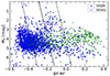 |
Fig. 1. Colour-magnitude diagram showing the 3084 objects included in Solano et al. (2022). Single stars are plotted as blue triangles, while binaries are plotted as green stars. The central line is the optimal hyperplane that best separates the two populations, computed using support vector machines (SVMs) with a linear kernel. The dashed lines are the positive and negative bounding hyperplanes that separate the soft margin. |
In Eq. (1) we show the decision function f(x) for the weighted-SVM (w-SVM) linear case, which determines the membership of a star to one of the classes in the feature space. It follows the general form f(x) = wT ⋅ x + b, where w is the vector of coefficients that weights the features, x1 and x2 the colour BP-RP and absolute magnitude MG respectively, and b is the bias term that adjusts the location of the decision function relative to the origin. This decision function represents a linear separation between classes single-binary, where the signs of the resulting values of f(x) indicate which class the star belongs to: if f(x) > 0, the point is classified as binary, and if f(x) < 0, it is classified as single:

Due to the nonlinear transformation induced by the RBF kernel, expressing the decision boundary as a simple linear equation is not feasible.
2.2. Extrapolation to a larger catalogue
We applied the two previous methods (w-SVM RBF and w-SVM linear), trained with the aforementioned sample of 3084 hot sds of Solano et al. (2022), to a larger catalogue which contains ∼39 800 hot subluminous star candidates selected in Gaia DR2 (Geier et al. 2019, see Figs. 3 and 4). When we use the w-SVM linear we get a single/binary ratio of 51/49 while if we use the w-SVM RBF we get 70/30.
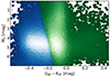 |
Fig. 3. Colour-magnitude diagram with the sample of 39 800 hot subluminous star candidates selected in Gaia DR2 by Geier et al. (2019) using a linear w-SVM classification. The stars in blue correspond to a prediction of singles, and those in green to binaries. The data are coloured using a point density function. |
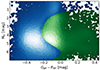 |
Fig. 4. Colour-magnitude diagram with the sample of 39 800 hot subluminous star candidates selected in Gaia DR2 by Geier et al. (2019) using a radial basis function (RBF) for the w-SVM classification (colours as in Fig. 3). |
Since we are testing candidates, all of the above proves to be effective for a first and raw classification and statistical separation of large amounts of stars into possible single-binaries, for a subsequent detailed analysis of the spectra using other techniques, as we show below. Even so, the prediction accuracy may decrease when extrapolating beyond the feature space region covered by the training samples (Wang et al. 2022). Combining photometry and spectroscopy for star classification offers advantages over only using spectra. It reduces initial complexity by employing less computationally intensive photometric data for a preliminary classification and enhances precision by leveraging complementary information from both data types, providing flexibility for optimizing each stage independently.
3. Single-binary classification of hot sds based on Gaia DR3 BP/RP spectroscopy using SOM and CNN
In the previous section, our investigation primarily delved into photometry. However, the transition to spectroscopy with Gaia’s BR/RP spectra was prompted by the need for more detailed insights into stellar characteristics. Spectroscopic data offer richer information, which are crucial for distinguishing between single and binary systems. Notably, the use of Gaia’s spectra for this purpose is novel, as previous studies have predominantly relied on photometric observations. Therefore, our exploration utilizing Gaia’s spectra for discriminating between single and binary stars fills a notable gap in the field, offering a promising avenue for enhanced stellar characterization. In the next sections, we address this by employing two techniques, Self-Organizing Maps (SOMs) and Convolutional Neural Networks (CNN), to effectively analyse Gaia’s BR/RP spectra. To train the SOM and CNN, we used 2815 objects of the Geier (2020) catalogue having binary/single classification in Solano et al. (2022) and with Gaia DR3 BP/RP spectra (De Angeli et al. 2023). The Gaia DR3 BP and RP spectra span the wavelength ranges of 330–680 nm and 640–1050 nm, respectively, with resolutions ranging from 100 to 30 for BP and from 100 to 70 for RP (De Angeli et al. 2023). To normalize these spectra, we divided each flux value by the maximum flux value within that spectrum. By doing this, we ensure that the highest flux value in each of the spectra is scaled to 1, while all other flux values are proportionally reduced, allowing a consistent comparison between different spectra.
Both the SOM and CNN techniques are purely data-driven. This means that their classification is only based on the numeric flux values in the spectra, with no additional input physics or other information about the nature of the spectra involved.
3.1. Pre-analysis of the spectra
To ensure that SOM and CNN will be trained on good quality data, initially we pre-analysed our BP/RP spectra with two different approaches: A Uniform Manifold Approximation and Projection (UMAP) method and the cosine similarity analysis.
The UMAP tool is a method to visualize similarities between high-dimensional data points in large datasets (McInnes et al. 2018). In our context, every spectrum is a 308 dimensional data point (one dimension for every wavelength bin in a spectrum) in a dataset of size 2815. In a UMAP projection, each of the high-dimensional data points is represented by a single point in a two-dimensional plane. The distance between two points in this plane is a measure of the similarity of the represented spectra. Close points in the UMAP projection represent similar spectra, while a large distance between points shows that the spectra are different from each other. Figure 5 shows the UMAP projection of our 2815 sample spectra. We can see that there is a variety of spectral shapes in our dataset, with an isolated group of 98 spectra. Our investigation of this group shows that all of them show atypically low flux values at wavelengths < 400 nm. These low flux values emerge during Gaia’s data reduction process and are not of physical origin (see e.g. van Leeuwen et al. 2022; De Angeli et al. 2023). We show in Sect. 5.2 that the difference between single and binary spectra increases towards larger wavelengths, and that they are indistinguishable at wavelengths < 400 nm. We concluded that for the single-binary classification, the spectral flux at these low wavelengths is not significant. Therefore, we decided to keep these 98 anomalous spectra for the training of our SOM and CNN. We also see in Fig. 5 that single and binary spectra cover the same space in the UMAP projection. There is a concentration of binary spectra along a filament in the projection, but this filament also contains a significant number of single spectra. Binary spectra are also found outside of the mentioned filament, distributed more or less uniformly among the single spectra. This UMAP approach is therefore not able to reliably classify individual, unlabelled spectra into single or binary.
 |
Fig. 5. UMAP projection of our 2815 sample spectra. Every data point in the map represents a spectrum. The colours indicate whether the spectrum has been classified as single or binary by VOSA. The dashed ellipse marks the position of the 98 anomalous spectra in the projection. The axis dimensions have no direct physical meaning. |
The cosine similarity measure is a different method to assess the similarity between data points in high-dimensional sets. We implemented the method with the SCIKIT-LEARN package (Pedregosa et al. 2011). To do this, we considered the 2815 normalized spectra as vectors and derived the cosine similarity by using the following Euclidean dot product formula (Eq. (2)),
where Ai and Bi are the i-th components of vectors A and B, respectively. For every pair of spectra in our dataset, this method returns a value between 0 (very dissimilar) and 1 (identical). We can average the cosine similarity values between a given spectrum and all other spectra, to find how similar this single spectrum is to the whole dataset. Outlier spectra will then have a low mean cosine similarity value. The vast majority of spectra (96%) have similarity values > 0.97, meaning that they are very similar to each other. Only a few spectra are dissimilar to the rest.
We compare the results from our cosine similarity analysis and the UMAP projection in Fig. 6. Here, we colour-code the data points in the UMAP by the mean cosine similarity for every spectrum. The colour-coding shows that the two methods agree well with each other: Spectra at the edges of the UMAP also have lower values of the mean cosine similarity. The 98 anomalous spectra, identified in the UMAP, also have low cosine similarity values. The average cosine similarity of the group of anomalous spectra is 0.971, while the average similarity of the rest of the spectra is 0.988. This comparison shows that the cosine similarity and UMAP analysis complement each other and are effective in finding outliers in a large set of spectra.
 |
Fig. 6. Same UMAP projection as in Fig. 5. The colour-coding indicates the mean cosine similarity of every projected spectrum. |
For future projects, we aim to apply SOM and CNN to sets of unlabelled spectra that are much larger than our current set of 2815. Then it will be impossible to visually inspect all spectra prior to the training. The cosine similarity and UMAP analysis will therefore be valuable tools to assess the quality of our initial dataset.
3.2. SOM classification based on the GDR3 BP/RP spectra
With the aim of classifying stars based on their nature, without any other a priori knowledge that could bias the results, we have used an unsupervised learning technique called Self-Organizing Maps (SOM). SOM is a technique that unifies the concepts of clustering and dimensionality reduction, since it groups objects based on their similarity and, in turn, performs a non-linear reduction of dimensionality by projecting the data into a certain number of groups, called neurons, and retaining the information on the distribution of the data in their topology. Each neuron has a prototype, that is the representative pattern of the objects that belong to that group, and normally the neurons are arranged in a two-dimensional structure,
The optimal configuration of the SOM, presented in this paper, is found to be around 100 clusters in a 10 × 10 lattice, and it has been trained for 200 iterations. We train the SOM on our sample of 2815 Gaia DR3 BP/RP spectra together with their classification from the Geier (2020) catalogue. We then analyse and visualize the SOM outputs with the Gaia Utility for the Analysis of self-organizing maps (GUASOM) (Fustes et al. 2014; Álvarez et al. 2022).
Figure 7 presents a visualization of the results obtained showing how the technique has been able to satisfactorily group the different types of stars using their spectra. Furthermore, by labelling the different neurons we can easily identify the region of neurons that mostly represents the binaries and the region of the single stars. Labelling is carried out by absolute majority; therefore, to determine the probabilities that each neuron has of representing a binary or a single star, Fig. 8 should be analysed.
 |
Fig. 7. Category plot, showing the representative label of each neuron according to classification given in Solano et al. (2022). |
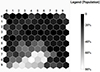 |
Fig. 8. Binary probability distribution showing the probability that each neuron represents a binary star. Lighter colours represent higher probabilities (see colour bar at right). |
 |
Fig. 9. Distribution of SOM output probabilities that spectra are binary. Top panel: Distribution of probabilities for spectra that have been labelled binary by VOSA. Bottom panel: Same as top panel, but for VOSA single spectra. The numbers in the plot show how many spectra fall above or below the 50% probability threshold. The green bars highlight the agreement between the SOM and VOSA labels; the red bars show the disagreement between the two methods. |
Figure 9 shows that our SOM method is able to identify single stars in our dataset with high accuracy. More than 97% of the VOSA single stars have been labelled correctly. This in turn means that the number of VOSA single stars that have wrongly been labelled binary by SOM is only 3%. We provide a more in-depth analysis of the prediction metrics in Sect. 4.
3.3. CNN classification based on the GDR3 BP/RP spectra
Convolutional neural networks have been successfully used to classify objects in large astronomical datasets. Examples are the morphological classification of galaxies based on 2D images (Khalifa et al. 2018) and the prediction of stellar spectral and luminosity classes from 1D spectra (Sharma et al. 2019). Tan et al. (2022) use a CNN to identify hot sds in a large sample of spectra of mixed spectral types from the LAMOST survey. We further specialize the CNN approach to classify subdwarf spectra into single and binary.
The convolution layers enable a CNN to identify extended features in input data. The network can then learn the connections between these features and the class of the object which is represented by the data. With network gradients it is possible to visualize the importance of different features in the input data on the network output class.
We trained a CNN to classify our sample of 2815 GDR3 BP/RP spectra into single and binary. Neural networks are a class of supervised machine learning techniques. Supervised techniques require a training set with pre-determined labels, from which the network can learn. In our case, this training set consists of GDR3 BP/RP spectra and their associated labels (these are single or binary). Once the training is finished, we can use the trained network to classify new, previously unlabelled spectra. Our trained CNN behaves like a function, that returns a value between 0 and 1 for every input spectrum. This value can be interpreted as a membership probability to the binary class.
For the training of our network, we used a set of 700 spectra and their VOSA labels. To avoid the complications that arise from training on imbalanced training data (see e.g. Krawczyk 2016), our training set contains as many binary stars as single stars. The number of available training spectra was therefore restricted by the relatively low number of spectra labelled as binary in our overall sample.
To monitor the learning progress of the network during the training, and to detect possible overfitting to the training set, we also constructed a validation set of 300 spectra and labels. This validation set is also balanced with respect to single and binary samples. Spectra from our overall sample were assigned at random to either the training set or validation set. We tested different network architectures and hyperparameters to optimize the performance of our CNN. The final architecture and the chosen hyperparameters are listed in Table 1.
Architecture and most important hyperparameters of our CNN.
The convolution layer is designed to identify features in the input spectra, such as absorption lines and positive or negative slopes. Based on these found features, the following dense layers calculate the output probability that a spectrum is binary. The optimal pixel values of the convolution filters and the weights and biases of the dense layer units (neurons) are learned during the network training phase (for more details about CNN architectures and training, see e.g. Indolia et al. 2018).
Our network has been trained for 200 epochs, using mini-batch training with a batch-size of 16. Training for more epochs does not significantly improve the training accuracy and leads to overfitting. For the network training, every network output with a value > 0.5 is assigned to the label binary. As the training progresses, the fraction of correctly labelled spectra increases. We show the improvement of the training and validation set accuracies during the 200 training epochs in Fig. 10. The labelling accuracies for the two sets increase together to a final value of ∼90%. This close match between the two sets shows that our CNN does not overfit to the training data at any point during the training.
 |
Fig. 10. Evolution of the accuracy of the network predictions during the training process. The validation set accuracy (orange) closely follows the training set accuracy (black), showing that the network does not overfit. |
When we use our trained network to classify our full sample of 2815 spectra (of which 558 are labelled binary by VOSA), the accuracy decreases to ∼85%. As can be seen from Fig. 11, the reason for this drop in accuracy is that our network wrongly labels some VOSA single spectra as binary.
 |
Fig. 11. Distribution of CNN output probabilities that spectra are binary. Top panel: Distribution of probabilities for spectra that have been labelled binary by VOSA. Bottom panel: Same as top panel, but for VOSA single spectra. The numbers in the plot show how many spectra fall above or below the 50% probability threshold. The green bars highlight the agreement of the CNN and VOSA labels; the red bars show the disagreement between the two methods. |
Network gradients have been used to show that CNNs can label stellar spectra in a physically meaningful way (for example, Ambrosch et al. 2023 and Nepal et al. 2023). These gradients describe how individual flux values in the input spectra influence the values of the CNN outputs. In our case, the network gradients show which parts of an input spectrum have the most influence on the probability for being binary. A positive gradient at a certain wavelength indicates that there is a positive correlation between flux value and output probability. The higher the flux at this wavelength, the higher the probability for being binary. Negative gradients indicate negative correlation between flux and output probability. Gradients are close to zero at parts of the spectrum that do not have an influence on the CNN output. Figure 12 shows the gradients for the probability of being binary together with an average spectrum from our sample. At lower wavelengths, the gradient is close to zero. This means that in this part of the spectra, our CNN cannot effectively identify features that help it to decide whether a spectrum is binary or not. At wavelengths larger than 700 nm however, the gradient is positive and increases steadily. We can therefore conclude that our network assigns binary probabilities based on the infrared flux in our GDR3 BP/BR spectra. This is consistent with how VOSA identifies binaries based on flux excess towards redder bands.
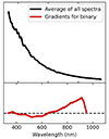 |
Fig. 12. Network gradients showing the sensitivity of our CNN to different parts of the input spectra. Top panel: Average of all GDR3 BP/RP spectra. Bottom panel: Network gradients for the prediction binary at every wavelength pixel. |
4. Evaluation and comparison of the prediction metrics for the different classification methods.
In our analysis, we adopted several key metrics to evaluate the performance of our classification models (see e.g. Stehman 1997). This has been done considering the VOSA classification as the true one. Thus, TP are the true positives, which occur when the model accurately predicts a binary while FP are the false positives, that is, when a binary is predicted incorrectly; on the contrary, the TN are the true negatives, which occur when a single is correctly predicted, while the false negatives (FN) occur when a single is predicted incorrectly. These metrics include the true positive rate (TPR) (Eq. (3)), which measures the proportion of binary stars correctly identified as such, and the true negative rate (TNR) (Eq. (4)), which measures the proportion of single stars correctly identified. Additionally, we assessed Accuracy (Eq. (5)), which represents the overall proportion of correctly classified instances, considering both binary and single stars. The Balanced Accuracy (Eq. (6)) accounts for the imbalance between the two classes by taking the average of TPR and TNR. The precision predictive value (PPV) (Eq. (7)) focuses on the proportion of correctly predicted binary stars among all predicted binary stars, while the negative predictive value (NPV) (Eq. (8)) focuses on the proportion of correctly predicted single stars among all predicted single stars. Lastly, the F1 Score (Eqs. (9) and 10) provides a balance between precision and recall, considering both the proportion of correctly predicted binary stars and the ability to capture all binary and single stars:


In Fig. 13 we present the confusion matrix, showcasing the true positives (binaries) and negatives (singles), along with the false positives and negatives, resulting from the predictions made by the four methods relative to the classification provided by VOSA. In Figs. A.1 and A.2 we compare the labels obtained with the 5 methods (including VOSA) with each other as a colour-coded matrix, where the number represents the common stars with the same label (true positives and negatives). For instance, based on these figures, it is evident that CNNs and linear w-SVMs are the most effective in identifying binaries (543 objects classified as binaries in common). In Table 2 we show the prediction quality metrics, containing the percentages of true labels with respect to those obtained individually with VOSA. These results represent the performance of each method’s classifications and how well they align with those of VOSA in classifying stars as binaries or singles based on photometry (SVM) and spectroscopy (SOM and CNN). As we can see, SVM (linear) and SVM (rbf) achieve similar True Positive Rates (TPR) around 68–70%, indicating their ability to correctly identify binary stars using photometric data. SOM shows a lower TPR of 42%, suggesting it may struggle more with binary classification based on spectroscopic data. In Fig. A.3, we present the classification results of SOMs and CNNs on a CMD, thus combining spectroscopy with photometry. As evident, single stars predominantly occupy the bluest region, while binaries are predominantly found in the redder region, as expected. It is notable that CNNs exhibit a superior capability in classifying binaries compared to SOMs, which appears more conservative. CNN demonstrates the highest TPR, 85%, indicating strong binary classification capabilities using spectroscopic information. True Negative Rates (TNR) are consistently high across all methods, ranging from 86% to 97%, indicating their proficiency in identifying single stars based on both photometric and spectroscopic data. Overall Accuracy rates vary between 83% and 89%, with CNN showing the highest accuracy, suggesting its effectiveness in both binary and single star classification using spectroscopic data. However, our sample of singles/binaries is unbalanced at approximately 80/20%. The balanced accuracy considers the balance between TPR and TNR, that is, the contribution of the two classes equally (50/50%), giving the same weight to the accuracy in the classification of both classes. We got values ranging from 78% to 87%, reflecting the overall performance in both binary and single star classification using photometric and spectroscopic data. Positive Predictive Value (PPV) ranges from 56% to 79%, indicating the proportion of correctly identified binary stars among all stars classified as binaries using photometric and spectroscopic data. Negative Predictive Value (NPV) ranges from 87% to 96%, showing the proportion of correctly identified single stars among all stars classified as singles using photometric and spectroscopic data. F1 Score (P), which considers both precision and recall, varies from 55% to 75%, providing a combined measure of binary classification performance using photometric and spectroscopic data. F1 Score (N) indicate strong performance across all methods in correctly classifying the negative (binary) instances, with values ranging from approximately 88% to 93%. All these metrics together offer insights into the effectiveness of each method in distinguishing between binary and single stars, with CNN exhibiting the most promising performance across multiple evaluation criteria when utilizing spectroscopic data.
 |
Fig. 13. Confusion matrix for the different classification methods. Each matrix displays the performance of a method in distinguishing between single and binary classes. The cells shaded in green represent true positive and true negative predictions, indicating correct classifications, while the cells shaded in red represent false positive and false negative predictions, indicating incorrect classifications. |
Prediction quality metrics for different methods with respect to VOSA.
We emphasize that to classify a star as single or binary in the methods described in this work, we have considered that the probability of belonging to one class is greater than 50%. However, to classify a star as single or binary robustly we recommend only considering those stars that agree on the classification by all methods or with a high probability in several of them. Upon analysing 2815 stars, we identified 260 objects that meet the criteria for binary classification based on all four of our photometric and spectroscopic methods, while 1947 are classified as single stars. This shows a strong concordance rate of 78% across all four classification techniques (linear and RBF SVMs based in photometry, as well as spectroscopy using SOM and CNNs), with a 22% discrepancy in classifications. This criterion of agreement in the classification offers statistical reliability, diminishes classification errors, ensures consistency among methods, and enhances the trustworthiness of result interpretation. In the appendix we provide an extract from the online table (Table A.1) with the predicted label by the different methods and probability of each object being binary. In the same table we also provide a column with a quality flag with values between 0-5, where a value of 0 means that all 5 methods classify the object as single and a value of 5 means that all 5 methods classify it as binary. It is worth mentioning again that each method tested has a different approach to the problem, so the SOM is an unsupervised method that does not know the labels “a priori”, while SVM and CNN are supervised methods. While for the SVMs we have used photometry, for the other methods we have used spectroscopy.
Finally, a statistical comparison was conducted among the probabilities of being a binary star across the spectroscopic methods. In Fig. A.4 we show the cumulative distribution function (CDFs) and the results of the Kolmogorov-Smirnov (K-S) statistic test (Kolmogorov 1933; Smirnov 1939) applied to the probability of being binary and computed using scipy.stats (Virtanen et al. 2020). The K-S test provides an objective measure of how similar or different these probability distributions are and allows the consistency to be evaluated between the results obtained by the two classification methods. Additionally, it can help to identify regions within the distributions where significant discrepancies exist. We obtained a good agreement between the probability distribution using both methods, with very low p-values (< 0.05). This means that there is a very low probability that those results occurred by random chance, and we have stronger evidence to reject the null hypothesis. We also found that the maximum absolute difference between the cumulative distributions of probabilities of being binary is at about P = 0.5. As we can see in Fig. A.4, the SOMs reach a probability of being binary > 0.5 at a higher density than the CNNs, which indicates that the latter classify more stars as binary than the former, which is more conservative in its predictions.
5. Possible unveiling of outliers in large Gaia DR3 spectra sets.
In this section, we explore further ways to analyse and categorize larger sets of spectra. When applying machine learning techniques to unlabelled spectra, it is important to understand the structure and internal properties of the full set. This allows us, for example, to identify outlier spectra or other special groups of spectra that may need to be treated separately. This type of pre-analysis enables us to interpret the outputs of our various ML techniques, specially when dealing with very large datasets. We tested this idea with a selected and well-known hot subdwarf sample with the objective of laying groundwork for future steps, as we aim at further analysing (in preparation, in a separate work) the ∼61 000 candidates identified by Culpan et al. (2022a), by means of their Gaia spectra, enabling us to initially distinguish objects that do not fit the hot sds profile.
5.1. The cosine similarity of single and binary spectra of a hot sds ’golden sample’.
In Sect. 3 we made a pre-analysis of the 2815 GDR3 BP/RP spectra, finding a small percentage of them as anomalous. In order to investigate these spectra in more detail, we chose a so-called golden sample of 88 targets, to which we applied the same technique. These well-defined hot sds are 35 binaries (from Solano et al. 2022) and 53 singles (from Drilling et al. 2013), which were selected as follows. Drilling et al. (2013) provided an MK (Morgan-Keenan)-like classification system which is still used as a reference for single hot sd spectral classification. Binary contamination was excluded from their study and the targets retained by the authors are considered a representative single hot subdwarfs and blue horizontal-branch stars sample. 53 objects out of their Table 1 were found to have Gaia DR3 BP/RP spectra and, therefore, suitable for our analysis. For the case of binary hot sds classification, we are not aware of a similar published system to the one provided by Drilling et al. (2013) for single objects. Therefore, we selected 35 binary hot sds from the work by Solano et al. (2022), with Gaia BP/RP spectra. That is to say, that, after a careful final data inspection, Solano et al. (2022) retained 42 targets with sufficiently good SEDs for two-body fitting attempts and for effective temperature determinations. Out of a cross-match of those 42 binaries with GDR3, we retained the above-mentioned 35 of them to have BP/RP spectra. For these selected hot sds, 53 singles from Drilling et al. (2013) and 35 binaries from Solano et al. (2022), we compared the 88 normalized Gaia DR3 BP/RP spectra with each other using the cosine similarity measure implemented using the SCIKIT-LEARN package (Pedregosa et al. 2011). To do this, we considered these 88 normalized spectra as vectors and derived the cosine similarity by using Eq. (2) as defined in Sect. 3. The results are shown in a colour-coded matrix in Fig. 14 for binaries and in Fig. 15 for singles. This similarity matrix provides a visual representation of the degree of similarity between each pair of spectra, highlighting patterns and relationships within the dataset. As can be seen, one star (LAMOSTJ112914.11+471501.7) stands out especially among the binaries and 4 stars (HD14829, Feige98, PG0304+184 and PG1510+635) among the singles, with a few more in between. For these, the mean value of the cosine similarity is significantly lower than the others (≤0.95), which indicates that the angle of the vectors that represent their spectra is greater and therefore they differ more from the others. LAMOSTJ112914.11+471501.7 had been classified by the SVMs and CNNs in the preceding sections as binary, which is in agreement with VOSA. Gaia’s spectra are reconstructed from a series of basis functions, and these deviations (which are not real) occasionally emerge, particularly in the spectra of the five stars under discussion. Thus, the cosine similarity method proves effective in detecting outliers or stars significantly different from the rest.
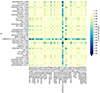 |
Fig. 14. Heatmap of 35 binary stars from a chosen subsample from Solano et al. (2022) and colour-coded according to their cosine similarity. |
 |
Fig. 15. Heatmap of 53 single stars from a chosen subsample from Drilling et al. (2013) and colour-coded according to their cosine similarity. |
After this, the next step is to inspect the spectra of those more differentiated stars, which is shown in Figs. A.5 to A.9. As we can see, those five stars fit into a common category, with characteristics that differentiate them. This is especially seen in the features at shorter wavelengths (λ < ∼400 nm) and because for larger intervals of the spectra, the flux is higher than the others. This leads us to classify the spectra into different categories according to their common features in their spectra.
Thus, in search of patterns within the spectra, we also used the UMAP technique to reduce the dimensionality of the similarity matrix (from 88 × 88 to a two-dimensional space) and then applied the Density-Based Spatial Clustering of Applications with Noise (DBSCAN) algorithm through the SCIKIT-LEARN package (Pedregosa et al. 2011) to perform clustering on the reduced data. This method is able of differentiating the spectra into several groups, which is shown in Fig. 16. As we can see, clusters 0 and 4, which are closest in the aforementioned Fig. 16, are characterized by having a decreasing spectrum at increasing wavelength, occupying the lowest fluxes compared to the others (Figs. A.10 to A.15). Then we have clusters 1, 2 and 3, with higher fluxes than clusters 0 and 4 at longer wavelengths, and more pronounced features below at around 400–450 nm. Cluster −1 would correspond to outlier or noise spectra, since they do not meet the criteria to be part of a cluster and they are difficult to classify. Finally, the 5 stars that we mentioned above with peculiar patterns would be included in cluster 2, which are characterized by having the highest fluxes, and in most of the cases with the special feature at short wavelengths (λ < ∼400 nm).
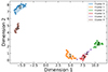 |
Fig. 16. Visualization of the similarity matrix reduced to two dimensions using UMAP. Groups of spectra that follow similar patterns are clustered using DBSCAN. |
When confronting the clusters with the detailed spectral types from Drilling et al. (2013), we observe distinct patterns in the distribution of spectral subtypes. Clusters 4 and 0 are dominated by early subtypes of sdO and sdB, as well as sdBN types. Clusters 1 and 3 features intermediate subtypes of sdB. Finally, cluster 2, with the highest mean fluxes, includes a variety of later subtypes of sdB and features sdA and sdOC types. Clusters with lower mean fluxes (4 and 0) contain more early subtypes, whereas clusters with higher mean fluxes (1, 3 and especially 2) include more late subtypes and varied types, according to Drilling et al. (2013) classification. The outliers are identified as blue horizontal branch (BHB) stars, distinguishable by their prominent Balmer lines that can be clearly detected in the low-resolution BP/RP spectra, as shown in the appendix figures.
5.2. The relative difference between singles and binaries.
On the other side, we conducted an analysis of spectral flux data for the 88 stars differentiating between single and binary stars. After processing the data, we computed the mean flux for the two types and calculated the relative difference. Visualization was achieved through a dual-axis plot, with the left axis displaying relative differences in percentages and the right axis showing mean flux values (see Fig. 17). Visualizing this relative difference across the spectrum helps to identify specific wavelengths where the two types of stars exhibit significant distinctions in their average flux values. The results show that the two classes become more differentiated as the wavelength increases, reaching relative differences of 60–80% beyond 800 nm. This is in agreement with what we saw in Sect. 3.3 for the whole sample and is consistent with the conclusions of Solano et al. (2022) using VOSA tools. The increasing trend in relative difference, coupled with a relatively constant difference between mean flux values of single and binary stars, may suggest heightened sensitivity or distinct spectral features at specific wavelengths. This indicates that certain wavelengths play a crucial role in distinguishing between single and binary stars, possibly due to pronounced spectral characteristics, the presence of specific chemical elements, or unique physical processes.Basically, what we are noticing here is the contribution of the secondary to the net flux. If the secondary is cooler, it will mostly emit at redder wavelengths, making this range quite appropriate to detect its contribution. The different nature of the companion on binary systems with hot sds would support this. The observed trends underscore the potential utility of certain wavelengths for discerning between binary and single stars based on their spectral features. Further exploration of these distinct regions can contribute to a more detailed understanding of the distinguishing factors between these stellar types.
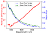 |
Fig. 17. Relative difference and mean fluxes between single and binary stars for our subsample of 53 singles and 35 binaries. |
6. Summary and conclusions
In this study we investigated the classification of single and binary hot subdwarf sources using various supervised and unsupervised classification criteria along with different Gaia DR3 datasets (both photometry and BP/RP spectroscopy). Our goal is to assess the extent to which we can replicate the classification provided in Solano et al. (2022) using VOSA and visual inspection of SEDs. Our findings reveal that, in general, all methods used demonstrates a high level of agreement with VOSA’s manual classification, achieving a reproducibility rate of near ∼70–90% for all cases. This suggests that SVM, SOM and CNN techniques can effectively classify single/binary bona-fide sources with accuracy comparable to human inspection using VOSA tools. The method based on spectroscopy using the CNN technique deserves special attention, which reaches 84.94% reproducibility for the detection of binaries. In global terms, the CNN reaches the best accuracy with near ∼90% of successes for the unbalanced and balanced samples. Techniques based on photometry using SVMs reach a ∼80% of accuracy. We also found an agreement of 78% in the classification using the four methods (through photometry and spectroscopy). The single/binary classification ratios achieved by the different methods are as follows: VOSA (80/20), linear w-SVM (75/25), RBF w-SVM (77/22), SOM (89/11) and CNN (75/25). Other techniques such as the cosine similarity and UMAP have also been applied, for pre-analysis of the 2815 sources with Gaia DR3 spectra and, to gain further insight, to a smaller and well-defined (88) subsample, proving very effective for the detection of outliers and peculiar spectra.
For future studies, we plan to leverage the Culpan et al. (2022a) sample, which provides improved accuracy and a larger dataset compared to Geier et al. (2019). The Culpan et al. (2022b) catalogue addresses issues with Gaia astrometry, particularly for close-by stars, thereby reducing the risk of misclassifying A-type MS stars as composite sdB binary candidates, as highlighted by Dawson et al. (2024). Taking advantage of this, our next step (in preparation) is to tackle the ∼61 000 candidates in Culpan et al. (2022a) to identify objects whose spectra significantly differ from those expected of singles or binaries. In extensive datasets, such as those in the aforementioned Culpan et al. (2022a), we anticipate significant contamination with DA white dwarfs, which also exhibit strong Balmer lines. Accurate identification of these DA white dwarfs is crucial. This pre-analysis aims to create a more refined subset of hot subdwarf candidates, which can then be analysed further using their GDR3 BP/RP spectra and the classification methods described in this paper. The methods above can also prove useful for finding misclassified objects. All techniques are complementary to each other and allow the comparison and/or the validation of results using different sources, whether photometry or spectroscopy.
Furthermore, our analysis highlights the challenges associated with classifying a large sample of sources where the composition is uncertain. While the classification accuracy is promising, caution is warranted when dealing with potentially contaminated samples. Future research could focus on refining classification techniques to mitigate the effects of contamination and improve the reliability of automated classification methods. Overall, this study contributes to the ongoing efforts in automating the classification of astronomical sources like single/binary hot sds, providing insights into the effectiveness of different methodologies and their applicability in large-scale surveys. Further investigations are able to explore additional techniques and validate the robustness of the classification results, especially in the presence of complex datasets and ambiguous source compositions.
Data availability
Full Table A.1 is available at the CDS via anonymous ftp to cdsarc.cds.unistra.fr (130.79.128.5) or via https://cdsarc.cds.unistra.fr/viz-bin/cat/J/A+A/691/A223
Figures A.1–A.15 are available in the Zenodo platform at https://doi.org/10.5281/zenodo.13841865
Acknowledgments
We sincerely thank the anonymous referee for her/his valuable guidelines and insightful comments, which have significantly enhanced the quality of this work. This research has made use of the Spanish Virtual Observatory (https://svo.cab.inta-csic.es) project funded by MCIN/AEI/10.13039/501100011033/ through grant PID2020-112949GB-I00. Also made use of GUASOM (Fustes et al. 2014; Álvarez et al. 2022), Scikit-learn Machine Learning (Pedregosa et al. 2011), NetworkX (Hagberg et al. 2008), Seaborn (Waskom 2021), TopCat (Taylor 2005), Pandas (The pandas development team 2020) and Matplotlib (Hunter 2007). This research has made extensive use of NASA’s Astrophysics Data System Bibliographic Services. This work has made use of data from the European Space Agency (ESA) Gaia mission, processed by the Gaia Data Processing and Analysis Consortium (DPAC). Funding for the DPAC has been provided by national institutions, in particular, the institutions participating in the Gaia Multilateral Agreement. This research has made use of the Simbad database and the Aladin sky atlas, operated at CDS, Strasbourg, France. The authors have also made use of the VOSA software, developed under the Spanish Virtual Observatory project supported by the Spanish MINECO through grant PID2020-112949GB-I00. Funding from Spanish Ministry project PID2021-122842OB-C22, Xunta de Galicia ED431B 2021/36 and PDC2021-121059-C22 is acknowledged by the authors. This work was funded by the Spanish MCIN/AEI/10.13039/501100011033 and European Union Next Generation EU/PRTR through grant PID2021-122842OB-C22 and the Horizon Europe [HORIZON-CL4-2023-SPACE-01-71], SPACIOUS project funded under Grant Agreement no. 101135205. CVV and AU thank the MW-Gaia COST Action “Revealing the Milky Way with Gaia” CA18104 for its support through a Short-term scientific mission (STSM) at the University of Vigo and to Erasmus+Staff for supporting a scientific visit of CVV to the aforementioned university. MAA, MM, RSG and JCD also acknowledge support from CIGUS CITIC, funded by Xunta de Galicia and the European Union (FEDER Galicia 2021-2027 Program) through grant ED431G 2023/01. This work is in the memory of Carlos Rodrigo (†), deceased during the preparation of this work.
References
- Aller, A., Miranda, L. F., Ulla, A., et al. 2013, A&A, 552, A25 [NASA ADS] [CrossRef] [EDP Sciences] [Google Scholar]
- Aller, A., Montesinos, B., Miranda, L. F., Solano, E., & Ulla, A. 2015, MNRAS, 448, 2822 [NASA ADS] [CrossRef] [Google Scholar]
- Álvarez, M. A., Dafonte, C., Manteiga, M., Garabato, D., & Santoveña, R. 2022, Neural Comput. Appl., 34, 1993 [CrossRef] [Google Scholar]
- Ambrosch, M., Guiglion, G., Mikolaitis, Š., et al. 2023, A&A, 672, A46 [NASA ADS] [CrossRef] [EDP Sciences] [Google Scholar]
- Ball, N. M., & Brunner, R. J. 2010, Int. J. Mod. Phys. D, 19, 1049 [Google Scholar]
- Bayo, A., Rodrigo, C., Barrado Y Navascués, D., et al. 2008, A&A, 492, 277 [NASA ADS] [CrossRef] [EDP Sciences] [Google Scholar]
- Bixler, J. V., Bowyer, S., & Laget, M. 1991, A&A, 250, 370 [NASA ADS] [PubMed] [Google Scholar]
- Boser, B. E., Guyon, I. M., & Vapnik, V. N. 1992, Proceedings ofthe Fifth Annual Workshop on Computational Learning Theory, COLT ’92 (New York, NY, USA: Association for Computing Machinery), 144 [CrossRef] [Google Scholar]
- Boyle, B. J., Fong, R., Shanks, T., & Peterson, B. A. 1990, MNRAS, 243, 1 [NASA ADS] [Google Scholar]
- Bu, Y., Zeng, J., Lei, Z., & Yi, Z. 2019, ApJ, 886, 128 [NASA ADS] [CrossRef] [Google Scholar]
- Cortes, C., & Vapnik, V. 1995, Mach. Learn., 20, 273 [Google Scholar]
- Cristianini, N., & Shawe-Taylor, J. 2000, An Introduction to Support Vector Machines and Other Kernel-based Learning Methods (Cambridge University Press) [CrossRef] [Google Scholar]
- Cui, X.-Q., Zhao, Y.-H., Chu, Y.-Q., et al. 2012, RAA, 12, 1197 [NASA ADS] [Google Scholar]
- Culpan, R., Geier, S., Reindl, N., et al. 2022a, A&A, 662, A40 [NASA ADS] [CrossRef] [EDP Sciences] [Google Scholar]
- Culpan, R., Geier, S., Reindl, N., et al. 2022b, VizieR Online Data Catalog: J/A+A/662/A40 [Google Scholar]
- Dawson, H., Geier, S., Heber, U., et al. 2024, A&A, 686, A25 [NASA ADS] [CrossRef] [EDP Sciences] [Google Scholar]
- D’Cruz, N. L., Dorman, B., Rood, R. T., & O’Connell, R. W. 1996, ApJ, 466, 359 [CrossRef] [Google Scholar]
- De Angeli, F., Weiler, M., Montegriffo, P., et al. 2023, A&A, 674, A2 [NASA ADS] [CrossRef] [EDP Sciences] [Google Scholar]
- Drilling, J. S., Jeffery, C. S., Heber, U., Moehler, S., & Napiwotzki, R. 2013, A&A, 551, A31 [NASA ADS] [CrossRef] [EDP Sciences] [Google Scholar]
- Dworetsky, M. M., Lanning, H. H., Etzel, P. B., & Patenaude, D. J. 1977, MNRAS, 181, 13P [CrossRef] [Google Scholar]
- Ferguson, D. H., Green, R. F., & Liebert, J. 1984, ApJ, 287, 320 [NASA ADS] [CrossRef] [Google Scholar]
- Fustes, D., Manteiga, M., Dafonte, C., et al. 2014, EAS Pub. Ser., 67–68, 373 [CrossRef] [EDP Sciences] [Google Scholar]
- Geier, S. 2020, A&A, 635, A193 [NASA ADS] [CrossRef] [EDP Sciences] [Google Scholar]
- Geier, S., Hirsch, H., Tillich, A., et al. 2011, A&A, 530, A28 [NASA ADS] [CrossRef] [EDP Sciences] [Google Scholar]
- Geier, S., Raddi, R., Gentile Fusillo, N. P., & Marsh, T. R. 2019, A&A, 621, A38 [NASA ADS] [CrossRef] [EDP Sciences] [Google Scholar]
- Geier, S., Dorsch, M., Pelisoli, I., et al. 2022, A&A, 661, A113 [NASA ADS] [CrossRef] [EDP Sciences] [Google Scholar]
- Green, R. F., Schmidt, M., & Liebert, J. 1986, ApJS, 61, 305 [NASA ADS] [CrossRef] [Google Scholar]
- Greenstein, J. L., & Sargent, A. I. 1974, ApJS, 28, 157 [Google Scholar]
- Hagberg, A. A., Schult, D. A., & Swart, P. J. 2008, in Proceedings of the 7th Python in Science Conference, eds. G. Varoquaux, T. Vaught, & J. Millman, 11 Pasadena, CA USA [Google Scholar]
- Han, Z., Podsiadlowski, P., Maxted, P. F. L., Marsh, T. R., & Ivanova, N. 2002, MNRAS, 336, 449 [Google Scholar]
- Han, Z., Podsiadlowski, P., Maxted, P. F. L., & Marsh, T. R. 2003, MNRAS, 341, 669 [NASA ADS] [CrossRef] [Google Scholar]
- Hartley, P., Flamary, R., Jackson, N., Tagore, A. S., & Metcalf, R. B. 2017, MNRAS, 471, 3378 [NASA ADS] [CrossRef] [Google Scholar]
- Hassanshahi, M. H., Jastrzebski, M., Malik, S., & Lahav, O. 2023, RAS Techn. Instrum., 2, 752 [NASA ADS] [CrossRef] [Google Scholar]
- Heber, U. 2009, ARA&A, 47, 211 [Google Scholar]
- Heber, U. 2016, PASP, 128, 082001 [Google Scholar]
- Huertas-Company, M., Rouan, D., Tasca, L., Soucail, G., & Le Fèvre, O. 2008, A&A, 478, 971 [NASA ADS] [CrossRef] [EDP Sciences] [Google Scholar]
- Huertas-Company, M., Aguerri, J. A. L., Bernardi, M., Mei, S., & Sánchez Almeida, J. 2011, A&A, 525, A157 [NASA ADS] [CrossRef] [EDP Sciences] [Google Scholar]
- Humason, M. L., & Zwicky, F. 1947, ApJ, 105, 85 [NASA ADS] [CrossRef] [Google Scholar]
- Hunter, J. D. 2007, Comput. Sci. Eng., 9, 90 [NASA ADS] [CrossRef] [Google Scholar]
- Indolia, S., Goswami, A. K., Mishra, S., & Asopa, P. 2018, Procedia Comput. Sci., 132, 679 [CrossRef] [Google Scholar]
- Kawka, A., Vennes, S., O’Toole, S., et al. 2015, MNRAS, 450, 3514 [Google Scholar]
- Khalifa, N. E., Hamed Taha, M., Hassanien, A. E., & Selim, I. 2018, in 2018 International Conference on Computing Sciences and Engineering (ICCSE), 1 [Google Scholar]
- Kilkenny, D., Heber, U., & Drilling, J. S. 1988, South Afr. Astron. Obs. Circ., 12, 1 [NASA ADS] [Google Scholar]
- Kleinman, S. J., Harris, H. C., Eisenstein, D. J., et al. 2004, ApJ, 607, 426 [NASA ADS] [CrossRef] [Google Scholar]
- Kolmogorov, A. 1933, Giornale dell’ Istituto Italiano degli Attuari, 4, 83 [Google Scholar]
- Kramer, M., Schneider, F. R. N., Ohlmann, S. T., et al. 2020, A&A, 642, A97 [NASA ADS] [CrossRef] [EDP Sciences] [Google Scholar]
- Krawczyk, B. 2016, Prog. Artif. Intell., 5, 221 [CrossRef] [Google Scholar]
- Kuiper, G. P. 1939, ApJ, 89, 548 [NASA ADS] [CrossRef] [Google Scholar]
- Latour, M., Hämmerich, S., Dorsch, M., et al. 2023, A&A, 677, A86 [NASA ADS] [CrossRef] [EDP Sciences] [Google Scholar]
- Lei, Z., Zhao, J., Németh, P., & Zhao, G. 2018, ApJ, 868, 70 [Google Scholar]
- Lei, Z., He, R., Németh, P., et al. 2023, ApJ, 942, 109 [CrossRef] [Google Scholar]
- Luo, Y.-P., Németh, P., Liu, C., Deng, L.-C., & Han, Z.-W. 2016, ApJ, 818, 202 [NASA ADS] [CrossRef] [Google Scholar]
- Luo, Y., Németh, P., Wang, K., Wang, X., & Han, Z. 2021, ApJS, 256, 28 [NASA ADS] [CrossRef] [Google Scholar]
- Luo, Y., Németh, P., Wang, K., & Pan, Y. 2024, ApJS, 271, 21 [NASA ADS] [CrossRef] [Google Scholar]
- Lynas-Gray, A. E. 2021, Front. Astron. Space Sci., 8, 19 [NASA ADS] [Google Scholar]
- Marton, G., Ábrahám, P., Szegedi-Elek, E., et al. 2019, MNRAS, 487, 2522 [Google Scholar]
- McInnes, L., Healy, J., Saul, N., & Grossberger, L. 2018, J. Open Source Software, 3, 861 [CrossRef] [Google Scholar]
- Mickaelian, A. M. 2008, AJ, 136, 946 [NASA ADS] [CrossRef] [Google Scholar]
- Moehler, S., Heber, U., & de Boer, K. S. 1990, A&A, 239, 265 [NASA ADS] [Google Scholar]
- Németh, P. 2020, Contrib. Astron. Obs. Skalnate Pleso, 50, 546 [Google Scholar]
- Nepal, S., Guiglion, G., de Jong, R. S., et al. 2023, A&A, 671, A61 [NASA ADS] [CrossRef] [EDP Sciences] [Google Scholar]
- Oreiro, R., Rodríguez-López, C., Solano, E., et al. 2011, A&A, 530, A2 [NASA ADS] [CrossRef] [EDP Sciences] [Google Scholar]
- Paczynski, B. 1980, Acta Astron., 30, 113 [NASA ADS] [Google Scholar]
- Pedregosa, F., Varoquaux, G., Gramfort, A., et al. 2011, J. Mach. Learn. Res., 12, 2825 [Google Scholar]
- Pelisoli, I., Vos, J., Geier, S., Schaffenroth, V., & Baran, A. S. 2020, A&A, 642, A180 [NASA ADS] [CrossRef] [EDP Sciences] [Google Scholar]
- Pérez-Fernández, E., Ulla, A., Solano, E., Oreiro, R., & Rodrigo, C. 2016, MNRAS, 457, 3396 [CrossRef] [Google Scholar]
- Ricker, G. R., Winn, J. N., Vanderspek, R., et al. 2015, J. Astron. Telesc. Instrum. Syst., 1, 014003 [Google Scholar]
- Rodrigo, C., Bayo Arán, A., Solano, E., & Cortés-Contreras, M. 2020, in XIV.0 Scientific Meeting (virtual) of the Spanish Astronomical Society, 181 [Google Scholar]
- Sahoo, S. K., Baran, A. S., Sanjayan, S., & Ostrowski, J. 2020, MNRAS, 499, 5508 [Google Scholar]
- Schaffenroth, V., Geier, S., Heber, U., et al. 2018, A&A, 614, A77 [NASA ADS] [CrossRef] [EDP Sciences] [Google Scholar]
- Schaffenroth, V., Pelisoli, I., Barlow, B. N., Geier, S., & Kupfer, T. 2022, A&A, 666, A182 [NASA ADS] [CrossRef] [EDP Sciences] [Google Scholar]
- Schaffenroth, V., Barlow, B. N., Pelisoli, I., Geier, S., & Kupfer, T. 2023, A&A, 673, A90 [NASA ADS] [CrossRef] [EDP Sciences] [Google Scholar]
- Scholkopf, B., Sung, K.-K., Burges, C. J. C., et al. 1997, IEEE Trans. Signal Process., 45, 2758 [CrossRef] [Google Scholar]
- Sharma, K., Kembhavi, A., Kembhavi, A., et al. 2019, MNRAS, 491, 2280 [Google Scholar]
- Silvotti, R., Schuh, S., Janulis, R., et al. 2007, Nature, 449, 189 [NASA ADS] [CrossRef] [Google Scholar]
- Smirnov, N. V. 1939, Bull. Moscow Univ., 2, 3 [Google Scholar]
- Solano, E., Ulla, A., Pérez-Fernández, E., et al. 2022, MNRAS, 514, 4239 [NASA ADS] [CrossRef] [Google Scholar]
- Stehman, S. V. 1997, Remote Sens. Environ., 62, 77 [NASA ADS] [CrossRef] [Google Scholar]
- Tan, L., Mei, Y., Liu, Z., et al. 2022, ApJS, 259, 5 [NASA ADS] [CrossRef] [Google Scholar]
- Taylor, M. B. 2005, ASP Conf. Ser., 347, 29 [Google Scholar]
- The pandas development team 2020, https://doi.org/10.5281/zenodo.3509134 [Google Scholar]
- Thejll, P., Ulla, A., & MacDonald, J. 1995, A&A, 303, 773 [Google Scholar]
- Thuillier, A., Van Grootel, V., Dévora-Pajares, M., et al. 2022, A&A, 664, A113 [NASA ADS] [CrossRef] [EDP Sciences] [Google Scholar]
- Ulla, A., & Thejll, P. 1998, A&AS, 132, 1 [NASA ADS] [CrossRef] [EDP Sciences] [Google Scholar]
- Uzundag, M., Krzesinski, J., Pelisoli, I., et al. 2024, A&A, 684, A118 [NASA ADS] [CrossRef] [EDP Sciences] [Google Scholar]
- Van Grootel, V., Pozuelos, F. J., Thuillier, A., et al. 2021, A&A, 650, A205 [NASA ADS] [CrossRef] [EDP Sciences] [Google Scholar]
- van Leeuwen, F., de Bruijne, J., Babusiaux, C., et al. 2022, Gaia DR3 documentation, Gaia DR3 documentation, European Space Agency; Gaia Data Processing and Analysis Consortium, https://gea.esac.esa.int/archive/documentation/GDR3/index.html [Google Scholar]
- Virtanen, P., Gommers, R., Oliphant, T. E., et al. 2020, Nat. Meth., 17, 261 [Google Scholar]
- Viscasillas Vázquez, C., Magrini, L., Spina, L., et al. 2023, A&A, 679, A122 [NASA ADS] [CrossRef] [EDP Sciences] [Google Scholar]
- Vos, J., Østensen, R. H., Degroote, P., et al. 2012, A&A, 548, A6 [NASA ADS] [CrossRef] [EDP Sciences] [Google Scholar]
- Vos, J., Østensen, R. H., Németh, P., et al. 2013, A&A, 559, A54 [NASA ADS] [CrossRef] [EDP Sciences] [Google Scholar]
- Vos, J., Østensen, R. H., Vučković, M., & Van Winckel, H. 2017, A&A, 605, A109 [NASA ADS] [CrossRef] [EDP Sciences] [Google Scholar]
- Vos, J., Németh, P., Vučković, M., Østensen, R., & Parsons, S. 2018, MNRAS, 473, 693 [NASA ADS] [CrossRef] [Google Scholar]
- Vos, J., Bobrick, A., & Vučković, M. 2020, A&A, 641, A163 [NASA ADS] [CrossRef] [EDP Sciences] [Google Scholar]
- Wang, C., Bai, Y., López-Sanjuan, C., et al. 2022, A&A, 659, A144 [Google Scholar]
- Waskom, M. L. 2021, J. Open Source Software, 6, 3021 [NASA ADS] [CrossRef] [Google Scholar]
- Zhang, X., & Jeffery, C. S. 2012, MNRAS, 419, 452 [NASA ADS] [CrossRef] [Google Scholar]
- Zhang, Y., & Zhao, Y. 2014, ASP Conf. Ser., 485, 239 [NASA ADS] [Google Scholar]
Appendix A: Complementary material
Figures A.1 - A.15 are available in the Zenodo platform at https://doi.org/10.5281/zenodo.13841865.
Classification labels for the different methods used in this work, where 0 means single and 1 binary. The probabilities of being binary and a flag that indicates the agreement between the different methods are also provided.
All Tables
Classification labels for the different methods used in this work, where 0 means single and 1 binary. The probabilities of being binary and a flag that indicates the agreement between the different methods are also provided.
All Figures
|
Fig. 1. Colour-magnitude diagram showing the 3084 objects included in Solano et al. (2022). Single stars are plotted as blue triangles, while binaries are plotted as green stars. The central line is the optimal hyperplane that best separates the two populations, computed using support vector machines (SVMs) with a linear kernel. The dashed lines are the positive and negative bounding hyperplanes that separate the soft margin. |
| In the text | |
 |
Fig. 2. Same as Fig. 1, but using a radial basis function (RBF). |
| In the text | |
|
Fig. 3. Colour-magnitude diagram with the sample of 39 800 hot subluminous star candidates selected in Gaia DR2 by Geier et al. (2019) using a linear w-SVM classification. The stars in blue correspond to a prediction of singles, and those in green to binaries. The data are coloured using a point density function. |
| In the text | |
|
Fig. 4. Colour-magnitude diagram with the sample of 39 800 hot subluminous star candidates selected in Gaia DR2 by Geier et al. (2019) using a radial basis function (RBF) for the w-SVM classification (colours as in Fig. 3). |
| In the text | |
|
Fig. 5. UMAP projection of our 2815 sample spectra. Every data point in the map represents a spectrum. The colours indicate whether the spectrum has been classified as single or binary by VOSA. The dashed ellipse marks the position of the 98 anomalous spectra in the projection. The axis dimensions have no direct physical meaning. |
| In the text | |
|
Fig. 6. Same UMAP projection as in Fig. 5. The colour-coding indicates the mean cosine similarity of every projected spectrum. |
| In the text | |
|
Fig. 7. Category plot, showing the representative label of each neuron according to classification given in Solano et al. (2022). |
| In the text | |
|
Fig. 8. Binary probability distribution showing the probability that each neuron represents a binary star. Lighter colours represent higher probabilities (see colour bar at right). |
| In the text | |
|
Fig. 9. Distribution of SOM output probabilities that spectra are binary. Top panel: Distribution of probabilities for spectra that have been labelled binary by VOSA. Bottom panel: Same as top panel, but for VOSA single spectra. The numbers in the plot show how many spectra fall above or below the 50% probability threshold. The green bars highlight the agreement between the SOM and VOSA labels; the red bars show the disagreement between the two methods. |
| In the text | |
|
Fig. 10. Evolution of the accuracy of the network predictions during the training process. The validation set accuracy (orange) closely follows the training set accuracy (black), showing that the network does not overfit. |
| In the text | |
|
Fig. 11. Distribution of CNN output probabilities that spectra are binary. Top panel: Distribution of probabilities for spectra that have been labelled binary by VOSA. Bottom panel: Same as top panel, but for VOSA single spectra. The numbers in the plot show how many spectra fall above or below the 50% probability threshold. The green bars highlight the agreement of the CNN and VOSA labels; the red bars show the disagreement between the two methods. |
| In the text | |
|
Fig. 12. Network gradients showing the sensitivity of our CNN to different parts of the input spectra. Top panel: Average of all GDR3 BP/RP spectra. Bottom panel: Network gradients for the prediction binary at every wavelength pixel. |
| In the text | |
|
Fig. 13. Confusion matrix for the different classification methods. Each matrix displays the performance of a method in distinguishing between single and binary classes. The cells shaded in green represent true positive and true negative predictions, indicating correct classifications, while the cells shaded in red represent false positive and false negative predictions, indicating incorrect classifications. |
| In the text | |
|
Fig. 14. Heatmap of 35 binary stars from a chosen subsample from Solano et al. (2022) and colour-coded according to their cosine similarity. |
| In the text | |
|
Fig. 15. Heatmap of 53 single stars from a chosen subsample from Drilling et al. (2013) and colour-coded according to their cosine similarity. |
| In the text | |
|
Fig. 16. Visualization of the similarity matrix reduced to two dimensions using UMAP. Groups of spectra that follow similar patterns are clustered using DBSCAN. |
| In the text | |
|
Fig. 17. Relative difference and mean fluxes between single and binary stars for our subsample of 53 singles and 35 binaries. |
| In the text | |
Current usage metrics show cumulative count of Article Views (full-text article views including HTML views, PDF and ePub downloads, according to the available data) and Abstracts Views on Vision4Press platform.
Data correspond to usage on the plateform after 2015. The current usage metrics is available 48-96 hours after online publication and is updated daily on week days.
Initial download of the metrics may take a while.