| Issue |
A&A
Volume 691, November 2024
|
|
|---|---|---|
| Article Number | A17 | |
| Number of page(s) | 14 | |
| Section | Stellar structure and evolution | |
| DOI | https://doi.org/10.1051/0004-6361/202451092 | |
| Published online | 25 October 2024 | |
Anomalously low-mass core-He-burning star in NGC 6819 as a post-common-envelope phase product
1
Department of Physics & Astronomy “Augusto Righi”, University of Bologna, via Gobetti 93/2, 40129 Bologna, Italy
2
INAF-Astrophysics and Space Science Observatory of Bologna, via Gobetti 93/3, 40129 Bologna, Italy
3
Department of Physics, University of Surrey, Guildford, Surrey GU2 7XH, UK
⋆ Corresponding author; This email address is being protected from spambots. You need JavaScript enabled to view it.
Received:
12
June
2024
Accepted:
14
August
2024
Abstract
Precise masses of red giant stars enable a robust inference of their ages, but there are cases where these age estimates are very precise but also very inaccurate. Examples are core-helium-burning (CHeB) stars that have lost more mass than predicted by standard single-star evolutionary models. Members of star clusters in the Kepler database represent a unique opportunity to identify such stars because they combine exquisite asteroseismic constraints with independent age information (members of a star cluster share a similar age and chemical composition). We focus on the single metal-rich (Z ≈ Z⊙) Li-rich low-mass CHeB star KIC4937011, which is a member of the open cluster NGC 6819 (turn-off mass of ≈1.6 M⊙, i.e. an age of ≈2.4 Gyr). This star has a lower mass by ≈1 M⊙ than expected for its age and metallicity, which might be explained by binary interactions or mass loss along the red giant branch (RGB). To infer formation scenarios for this object, we performed a Bayesian analysis by combining the binary stellar evolutionary framework BINARY_C V2.2.3 with the dynamic nested-sampling approach contained in the DYNESTY V2.1.1 package. We find that this star probably is the result of a common-envelope evolution (CEE) phase during the RGB stage of the primary star in which the low-mass (< 0.71 M⊙) main-sequence companion does not survive. The mass of the primary star at the zero-age main sequence is in the range [1.46, 1.71] M⊙, with a log-orbital period in the range [0.06, 2.4] log10(days). During the CEE phase, ≈1 M⊙ of material is ejected from the system, and the final star reaches the CHeB stage after helium flashes as if it were a single star with a mass of ≈0.7 M⊙, which is what we observe today. Although the proposed scenario is consistent with photometric and spectroscopic observations, a quantitative comparison with detailed stellar evolution calculations is needed to quantify the systematic skewness of the radius, luminosity, and effective temperature distributions towards higher values than observations.
Key words: stars: evolution / stars: fundamental parameters / stars: horizontal-branch / stars: interiors / stars: mass-loss / stars: oscillations
© The Authors 2024
 Open Access article, published by EDP Sciences, under the terms of the Creative Commons Attribution License (https://creativecommons.org/licenses/by/4.0), which permits unrestricted use, distribution, and reproduction in any medium, provided the original work is properly cited.
This article is published in open access under the Subscribe to Open model. This email address is being protected from spambots. You need JavaScript enabled to view it. to support open access publication.
1. Introduction
The advent of the space mission Kepler has enabled us to study the oscillation spectra of tens of thousands of red giant stars in great detail, and thus, to constrain their internal structures, properties, and evolutionary phases. These asteroseismic constraints, coupled with information on photospheric chemical abundances and temperature, have also enabled us to precisely measure their radii and masses (De Ridder et al. 2009; Hekker et al. 2011; Huber et al. 2011; Miglio et al. 2013; Stello et al. 2013; Mosser et al. 2014; Yu et al. 2018; García & Ballot 2019; Kallinger 2019).
Precise masses of red giant stars enable a robust inference of their ages (Anders et al. 2016; Casagrande et al. 2016; Pinsonneault et al. 2018; Silva Aguirre et al. 2018; Miglio et al. 2021; Montalbán et al. 2021), but in some cases in the field and in open star clusters, these estimates are significantly different from the age predicted by standard single-star evolutionary models. For example, the masses of some members of open clusters are higher than the observed average mass for their evolutionary phase (Brogaard et al. 2016, 2018, 2021; Handberg et al. 2017). This means that these stars appear to be younger than they actually are, and this in turn means that they must have experienced mass transfer or merger events in the past (Izzard et al. 2018). Despite potential insights from observations that could assist in distinguishing between different formation scenarios (Brogaard et al. 2018), the evolutionary history of many observed systems with masses that deviate from their expected mass remains uncertain. The limited support from other stars in the age determination makes it challenging to identify non-standard evolutionary paths for field stars. An exception to this is the thick disc, which has a well-defined turn-off mass that allows us to track the evolutionary history of these stars (Chiappini et al. 2015; Martig et al. 2015; Izzard et al. 2018; Grisoni et al. 2024).
While systems are observed with masses that are significantly higher than the average mass in the cluster for their evolutionary phase, the opposite is true as well. The mass of some red giant members of open clusters is lower than the observed average mass for their evolutionary phase (Handberg et al. 2017; Brogaard et al. 2021). When we consider their mass and metallicity, they have lost more mass than expected, most likely via interaction with a companion star (Li et al. 2022; Bobrick et al. 2024) or because of mass loss along the red giant branch (RGB). Undermassive stars like this have also been observed in the field (Miglio et al. 2021; Li et al. 2022; Matteuzzi et al. 2023). Some of them are low-mass core-helium-burning (CHeB) stars that are located in the colour-magnitude diagram between RR Lyrae and red clump (RC) stars, that is, they are red horizontal branch (rHB) stars. By modelling their structure and pulsation spectra, Matteuzzi et al. (2023) found that these low-mass objects have a helium-core mass of ≈0.5 M⊙ and a hydrogen-rich envelope of ≈0.1 − 0.2 M⊙, that is, the envelopes of these stars are less massive than those of other stars in the same evolutionary phase and with similar metallicity, but they are slightly more massive than the RR Lyrae stars with a similar metallicity. This means that these undermassive stars are partially stripped, probably as a result of a past binary interaction. The investigation of plausible formation scenarios for these stars is critical to constrain their actual ages better and to potentially provide another piece of the puzzle in the sequence between RC stars, metal-rich RR Lyrae and subdwarf B (sdB) stars, or other stripped stars.
In binary stars, mass transfer is possible by direct Roche-lobe overflow (RLOF) or by wind mass loss (see De Marco & Izzard 2017, for a review). When mass is transferred from red giant stars and low-mass main-sequence (MS) stars on a dynamical timescale, the companion may be engulfed, and a common-envelope evolution begins (CEE; e.g. Paczyński 1976; Ivanova et al. 2013; Röpke & De Marco 2023). This can occur when mass transfer is unstable, that is, the transfer of mass by the donor leads to an increase in the mass-transfer rate. Whether the mass transfer becomes unstable is usually determined based on a critical mass ratio, qcrit, between the primary mass and the companion mass. When the system exceeds this mass ratio (q1 > qcrit, Hurley et al. 2002), it will undergo unstable mass transfer followed by a CEE. At this stage, drag forces transfer part of the orbital energy to the common envelope (CE), which shrinks the orbit and ejects at least part of the CE (Shima et al. 1985; Kim 2010; MacLeod & Ramirez-Ruiz 2015; Ohlmann et al. 2016; Chamandy et al. 2019; Reichardt et al. 2019; Sand et al. 2020). The consequence of this CE phase is that stars either merge or end up much closer than before this phase. The easiest way to model the CEE is using the α-formalism (van den Heuvel 1976; Webbink 1984; Livio & Soker 1988; de Kool 1990; Han et al. 1994; Dewi & Tauris 2000; Xu & Li 2010a,b; Ivanova & Chaichenets 2011; Wang et al. 2016), also called the energy formalism. This formalism can be described by the following equation:
 (1)
(1)
where
 (2)
(2)
and
 (3)
(3)
are the binding energy of the envelope of the primary star (the donor star) and the difference in orbital energy after and before the CEE, respectively. Ebind depends on the mass (m1), the envelope mass (m1, env), and the Roche-lobe radius (R1) of the primary star, and it also contains a numerical factor λce that characterises the central concentration of the envelope. ΔEorb also depends on the core mass of the primary star (m1, core = m1 − m1, env), the mass of the companion star (the accretor star), and on the orbital separation before (ai) and after (af) the CEE. Finally, αce indicates the fraction of orbital energy that is converted into energy that is used to eject the envelope. It therefore is the efficiency of the CE ejection. Unfortunately, there are no direct observations of CEE events with which we would be able to constrain λce and αce. Nonetheless, observations of post-CEE systems and 3D hydrodynamical simulations suggest that the value of αce is not universal and depends on many factors, such as the donor mass, the mass ratio, and the evolutionary stage (Taam & Sandquist 2000; Podsiadlowski et al. 2003; Politano 2004; De Marco et al. 2011; Davis et al. 2012; Iaconi & De Marco 2019; Belloni et al. 2024). Moreover, many works (Han et al. 1994; Dewi & Tauris 2000, 2001; Podsiadlowski et al. 2003; Webbink 2008; Xu & Li 2010a,b; Wong et al. 2014) suggested that λce varies as the star evolves and significantly deviates from a constant value. However, from an analysis of Eqs. (1), (2) and (3), it is evident that the properties of the post-CEE system do not change when the product αce ⋅ λce is held constant. Despite our limited understanding of the variables λce and αce, we can effectively constrain the post-CEE phase by using αce ⋅ λce. Conversely, a better knowledge of the post-CEE phase gives us a constraint on the possible αce ⋅ λce values.
Members of star clusters observed by the Kepler space telescope represent a unique opportunity to constrain formation channels of undermassive stars because they combine exquisite asteroseismic constraints with age information: The members of a star cluster share a similar age and chemical composition. In this paper, we focus on the red giant star KIC4937011, which is a member of the Galactic star cluster NGC 6819 and has a turn-off mass of ≈1.6 M⊙ (i.e. an age of ≈2.4 Gyr, Burkhead 1971; Lindoff 1972; Auner 1974; Rosvick & Vandenberg 1998; Kalirai et al. 2001; Basu et al. 2011; Yang et al. 2013; Jeffries et al. 2013; Bedin et al. 2015; Brewer et al. 2016). Based on the scaling relation between the mean large frequency separation and the frequency of maximum power, Handberg et al. (2017) determined that KIC4937011 has a mass of 0.71 ± 0.08 M⊙. This value is consistent within the errors with the mass calculated using the scaling relation involving the luminosity and the frequency of maximum power (Matteuzzi et al. 2023). Additionally, the analysis of the asymptotic period spacing of the dipole modes indicates that KIC4937011 is currently in the RC phase (Matteuzzi et al. 2023). Based on spectroscopy (Anthony-Twarog et al. 2013; Carlberg et al. 2015; Lee-Brown et al. 2015), we know that it is a single star with near-solar metallicity, a high lithium and oxygen content, and a rotational velocity of 8.3 ± 0.3 km/s (i.e. a higher value than the other red giant stars in this cluster). The mass of this star is lower by ≈1 M⊙ than the average mass of RC stars in NGC 6819 (i.e. 1.64 M⊙, Handberg et al. 2017), which could be explained by binary interactions.
The paper is organised as follows. We briefly describe the observational properties of KIC4937011 in Sect. 2. In Sect. 3 we describe the theoretical framework that permits us to predict the formation channel, and how we simulated binary interactions. In Sect. 4 we present our results, namely the most credible formation channels for this star, which is the consequence of a common-envelope evolution phase in which the companion does not survive. Section 5 concludes the paper.
2. Observational data
In Sect. 1 we stated that KIC4937011 is an RC member of the open cluster NGC 6819 (HRD in Figure 1, observational properties in Table 1). This is suggested by its radial velocity (Hole et al. 2009; Anthony-Twarog et al. 2013; Carlberg et al. 2015), CMD position (Anthony-Twarog et al. 2013), and proper motion (Gaia Collaboration 2016, 2023; Babusiaux et al. 2023). This allows us an independent estimation of the age of KIC4937011 regardless of its mass. We use the age estimate 2.38 ± 0.05 ± 0.22 Gyr1, which is based on eclipsing binaries of Brewer et al. (2016), but with an error of 0.27 Gyr2 (Sect. 3.2).
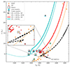 |
Fig. 1. HRD of NGC 6819 showing RC and RGB member stars. Except for standard single stars, some are members of binary systems, some are overmassive stars, and one star (KIC4937011) is undermassive. The solid lines show evolutionary tracks from the RGB phase until the first thermal pulse in the AGB phase for a 1.60 M⊙ and a 2.50 M⊙ star with solar metallicity, and the dotted line represents a 0.70 M⊙ star with solar metallicity from the beginning of the CHeB stage until the first thermal pulse in the AGB phase. KIC4937011 is dimmer and cooler than other member stars at the same evolutionary stage, and it would be compatible with a 1.60 M⊙ RGB star if we had no information about its evolutionary state and mass. For a full description of the models used in the figure, see Handberg et al. (2017). |
The metallicity of the cluster is similar to that of the Sun (Rosvick & Vandenberg 1998; Anthony-Twarog et al. 2014; Lee-Brown et al. 2015; Slumstrup et al. 2019), but other works suggested super-solar metallicities ([Fe/H] = 0.09 ± 0.03, Bragaglia et al. 2001). This is in line with the metallicity of KIC4937011, which is approximately solar ([Fe/H] = 0.04, Carlberg et al. 2015; [Fe/H] = −0.05, Lee-Brown et al. 2015). We used a metallicity Z = 0.02 for KIC4937011 (Sect. 3.2). The observed 12C/14N of KIC4937011 is consistent with its other more massive (i.e. ≈ 1.64 M⊙) counterparts in the RC phase, although the lower the mass, the higher 12C/14N is expected in a star that evolves in isolation (^12C/^14N > 3 for such a low-mass, metal-rich star, Salaris et al. 2015). Past mass-transfer events may provide an explanation for the peculiar 12C/14N observed in the envelope of KIC4937011. The envelope might originate from a star that was more massive during its first dredge-up than the current KIC4937011 (Hekker & Johnson 2019; Tayar et al. 2023).
Handberg et al. (2017) derived masses in NGC 6819 in the RGB and RC phases using asteroseismic data from Kepler. They obtained average masses of 1.61 ± 0.02 M⊙ and 1.64 ± 0.02 M⊙, respectively. This means that the integrated mass loss in the RGB phase in this cluster is compatible with a Reimers mass-loss law (Reimers 1975; Kudritzki & Reimers 1978) with an efficiency ηRGB = 0.1. However, the mass of KIC4937011 is lower by almost 1 M⊙ than that of its other counterparts in the RC phase. As a result, an efficiency ηRGB > 1 is required in order to explain the isolated evolution of this star. A high efficiency like this is highly improbable because it far exceeds the average value measured in NGC 6819. Therefore, it is unlikely that mass loss in the RGB phase through winds alone can account for the mass discrepancy observed in KIC4937011. Carlberg et al. (2015) proposed an interaction between a ≈1.7 M⊙ red giant star and a brown dwarf with a mass of 45 MJup to explain the enrichment in lithium [A(Li) = 12 + log(NLi/NH) = +2.3 dex, Anthony-Twarog et al. 2013] and the loss of almost 1 M⊙. However, alternative explanations exist for the observed Li-enrichment in red giant stars. Some observations suggested that R-stars with a similar chemical composition and lithium content may have interacted with a companion star instead of a brown dwarf (Zamora et al. 2006). Another possibility is that lithium-rich RC stars could have been created through the merging of a helium white dwarf (HeWD) star and a RGB star (Zhang et al. 2020). Several mechanisms have been proposed to account for the Li-enrichment in red giant stars, including planet or brown dwarf engulfment (Ashwell et al. 2005; Aguilera-Gómez et al. 2016a,b), accretion from an asymptotic giant branch (AGB) star or a nova (José & Hernanz 1998), and the Cameron & Fowler (1971) mechanism with some additional mixing (Denissenkov & Herwig 2004; Guandalini et al. 2009; Denissenkov 2010; Aguilera-Gómez et al. 2023), such as the HeWD-RGB merger mentioned above. Therefore, the lithium content alone is not a reliable indicator for distinguishing between formation channels. However, considering all available pieces of information, we need to incorporate binary interactions into evolutionary models of KIC4937011.
Carlberg et al. (2015) performed multiple checks to determine whether the spectroscopic analysis is affected by either a companion to the Li-rich star or an unrelated background object. They reported that the radial velocity is constant within 0.1 − 0.2 km/s in nearly one month of observations. Even when they considered 20 years of observations with other surveys, they did not obtain variations in its radial velocity. They also searched for a secondary spectrum, but did not identify any significant secondary peaks. Furthermore, there is no indication of infrared excess, which is observed in other Li-rich red giant stars (Rebull et al. 2015; Mallick et al. 2022). Even the currently available Gaia-DR3 astrometry data (non-single star processing in Halbwachs et al. 2023) lack evidence of companion stars. We also tested the non-single star hypothesis using the FIDELITY_V2 table (Rybizki et al. 2022) and the RUWE value3. All this information together suggests that KIC4937011 has no companion.
3. Bayesian inference of formation scenarios
In this section, we describe the Bayesian approach we adopted to infer the most probable formation scenario for KIC4937011, for which we used an evolutionary code for binary stars (Sect. 3.1) coupled with a Monte Carlo (MC) method (Sect. 3.2).
3.1. Evolutionary code for binary stars
The software BINARY_C V2.2.34 (Izzard et al. 2004, 2006, 2009, 2018; Izzard & Jermyn 2023) makes synthetic populations of single, binary, and multiple stars. It is based upon the code called binary star evolution (BSE) (Hurley et al. 2002), which uses analytic fits to rapidly follow the properties of a system as a function of time (Hurley et al. 2000). In addition, BINARY_C V2.2.3 rapidly calculates nucleosynthetic yields from these synthetic populations, adopting the supernova yields from massive stars from Woosley & Weaver (1995), Chieffi & Limongi (2004), and adopting first, second, and third dredge-up and thermally pulsing asymptotic giant branch (TPAGB) prescriptions from Izzard et al. (2006), which are based on Karakas et al. (2002). These prescriptions are very useful for globular cluster and Galactic chemical evolution simulations (Izzard et al. 2018; Yates et al. 2024). The physics implemented in the code (De Marco & Izzard 2017, for a review about relevant physical processes in binary systems) is mainly described in the papers cited above. The code allows the incorporation of alternative models beyond those used in the BSE code, such as different RLOF (Claeys et al. 2014), wind Roche-lobe overflow (WRLOF; Abate et al. 2013, 2015), accretion and thermohaline mixing (Stancliffe et al. 2007; Izzard et al. 2018), supernovae (Boubert et al. 2017a,b), tides (Siess et al. 2013), rejuvenation (de Mink et al. 2013; Schneider et al. 2014), stellar rotation (de Mink et al. 2013), stellar lifetimes (Schneider et al. 2014), CEE (Wang et al. 2016), and circumbinary discs (Izzard & Jermyn 2023). This algorithm operates about 107 times faster than full evolution and nucleosynthesis calculations, which makes it very useful for a Bayesian approach to parameter estimation.
We adopted a Python interface to BINARY_C V2.2.3, BINARY_C-PYTHON V0.9.65 (Hendriks & Izzard 2023). We mainly adopted the binary-physics prescriptions of the BSE code, but the model of the properties of the AGB comes from Karakas et al. (2002), the RLOF modelling onto a white dwarf from Claeys et al. (2014), and the critical mass ratios qcrit from Table 2.
Critical mass ratio qcrit for stable RLOF for different types of donor stars in the case of a non-degenerate and a degenerate accretor.
We fixed to 0.5 the fraction of the recombination energy in the CE that participates in the ejection of the envelope (i.e. λionisation = 0.5 in BINARY_C V2.2.3), and we considered αce ⋅ λce to be a single free parameter of the model. We forced a first dredge-up in the Hertzsprung gap (HG) and RGB stars that undergo a CEE phase, but not for MS stars, because the dynamical mixing effects owing to the spiral-in process are assumed to completely mix the envelope in red giant stars (Izzard et al. 2006). Furthermore, we did not include mass loss enhanced by rotation, tides, and He flashes. We also ignored thermohaline mixing, WRLOF, and the lithium abundance change over time.
3.2. Monte Carlo simulations
To constrain binary systems that best explain the current state of KIC4937011, we need to efficiently estimate the posterior of a set of parameters for a given model obtained with BINARY_C V2.2.3 and BINARY_C-PYTHON V0.9.6. We used the dynamic nested sampling approach contained in the DYNESTY V2.1.16 package (Speagle 2020).
The initial conditions of all MC simulations are a binary system formed by zero-age main-sequence (ZAMS) stars with circular orbits, Z = 0.02 and ηRGB = 0.1, where we choose the metallicity and mass loss to be compatible with observations (Sect. 2). Our main results do not change when we allowed Z and/or ηRGB to vary freely within the observational uncertainties. The main difference is that the density distributions become broader and less predictive. We did not consider initially eccentric binaries because the evolution of close binary populations is almost independent of the initial eccentricity (Hurley et al. 2002).
We used uniform priors for αce ⋅ λce (Sects. 1 and 3.1), the logarithm7 of the initial period, log P0, and the initial mass ratio, qZAMS = M2, ZAMS/M1, ZAMS. For the initial mass of the primary star, M1, ZAMS, we employ the probability density distribution of Chabrier (2003)8. We calculated the likelihood function given the current evolutionary phase (CHeB), mass (M1, CHeB = 0.71 ± 0.08 M⊙) and age (tage = 2.38 ± 0.27 Gyr) of the star (Sects. 1 and 2). For more details on the likelihood we used and the intervals chosen for our priors, we refer to Appendix A and Table A.1.
In Fig. 2 the corner plot shows the age and primary mass density distributions of our MC simulations at the CHeB stage (see also Table 1), compared with the observed values for KIC4937011 (red lines). Our modelling correctly fits the observed current age and mass of KIC4937011 within the errors.
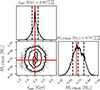 |
Fig. 2. Corner plot showing the age and primary mass density distributions at the CHeB stage for the full sample as described in Sect. 3.2. The contours refer to the 1, 2, and 3σ credible regions. The observed values for KIC4937011 are plotted in red (see also Table 1). We see that our modelling correctly fits, within errors, the observed current age and mass of KIC4937011. As explained in Appendix A, we take as the reference time for the CHeB of each MC simulation the age that gives the highest likelihood. |
4. Results
In this section, we present significant results derived from our Monte Carlo simulations (Sect. 4.1), and we discuss the most credible formation channel (Sect. 4.2).
4.1. Formation channels constrained by age and mass observations
Figure 3 shows the estimated posterior density distributions of Monte Carlo simulations discussed in Sect. 3.2 and presented in Table 1.
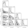 |
Fig. 3. Corner plot showing the posterior density distributions of the MC simulations described in Sect. 3.2. The contours refer to 1, 2, and 3 σ. |
A strong anti-correlation is observed between the product αce ⋅ λce and log P0, with a Pearson correlation coefficient of approximately −0.69. There are also weaker anti-correlations between log P0 and the other parameters. Equation (1) indicates that as the period increases, so does the orbital radius, while the surface gravity of the CE decreases, requiring a lower αce for the mass ejection. This suggests that certain areas of the log P0 − αce ⋅ λce plane can be excluded (Figure 3 and Table 1), but we are unable to provide stricter constraints on the individual values of log P0 and αce ⋅ λce. Furthermore, αce ⋅ λce here tends to higher values than suggested by other systems (Sect. 1). A plausible physical interpretation for this phenomenon is related to recombination energy. Specifically, high αce ⋅ λce values can be obtained when αce is constrained to values below one, and λce is calculated according to the Wang et al. (2016) prescriptions, using a high λionisation value. Nonetheless, we cannot rule out the influence of additional energy sources, including dust formation or nuclear burning, that occur during the CEE phase. They may also contribute to the observed high αce ⋅ λce values.
Our estimated M1, ZAMS (Figure 3 and Table 1) is slightly higher than but still consistent with the observed average mass of RGB stars in NGC6819 (1.61 ± 0.02 M⊙, Handberg et al. 2017). This implies that an RGB star with a mass of 1.87 M⊙ (i.e. the upper limit of our 68% credible interval for M1, ZAMS) would begin the RGB phase about 0.82 Gyr9 earlier than the current RGB stars in NGC6819. Therefore, any binary interaction and evolution that occurred between a primary RGB star and a companion should last less than ≈1 Gyr to be consistent with the observations. Moreover, the qZAMS posterior distribution lower limit in the 99.7% credible interval is very close to the lower limit of our prior distribution (Table A.1), and limits in the prior below 0.08 M⊙ are probably necessary for the companion mass.
4.1.1. Common-envelope phases create distinct pathways
In this section, we summarise the results concerning the number of CEE phases up to the CHeB stage of the primary star for the full sample. Every MC simulation considered (i.e. 65 225 simulations) had one CEE phase, and a negligible percentage (0.006%, i.e. 4 out of 65 225 simulations) had two. This implies that our modelling predicts that KIC4937011 is the product of a post-common-envelope phase. The majority of the binary systems (i.e. 99.92%) evolves without mass transfers until the primary star is in the subgiant or in the RGB phase and the companion in the MS phase. At this point, an unstable mass transfer begins, leading to a CEE phase and to the shrinkage of the orbits (Sect. 1). The loss of orbital energy causes the probability for another CEE phase to decrease significantly. Finally, in all our sample of MC simulations, the companion star merges with the primary star and leaves as the final product a single CHeB star. This is in line with the observations (Sect. 2).
4.1.2. Physical properties of the primary star
In Fig. 4 and Table 1 we present the helium-core mass, radius, luminosity, and effective temperature posterior density distributions of the primary star at the CHeB stage estimated by the MC simulations. The helium-core masses of the primary stars in our simulations lie in the 99.7% credible interval [0.32, 0.60] M⊙. Moreover, panel (a) shows three main peaks: at around 0.32 M⊙, 0.47 M⊙, and 0.52 M⊙. The first helium-core mass peak is expected for a secondary clump star and the second peak for a RC star (Girardi 2016). However, helium-core masses above ≈0.50 M⊙ are expected during the early asymptotic-giant branch (EAGB) stage and not during the CHeB stage. These high helium-core masses lead to much higher radii (> 15 R⊙) and luminosities (> 100 L⊙) than expected of CHeB stars of mass ≈0.7 M⊙, and they also lead to effective temperatures well below 4500 K. Moreover, these high luminosities would not be consistent with the behaviour of the mixed dipole modes observed in KIC4937011. It is worth noting that BINARY_C V2.2.3 is based on the Pols et al. (1998) evolutionary models, which predict higher radii, luminosities, and effective temperatures for these low-mass CHeB stars than more recent evolutionary models (Girardi 2016). These systematic effects must be taken into account for a comparison with observations (Sect. 4.2.1).
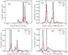 |
Fig. 4. Helium-core mass (panel a), radius (panel b), luminosity (panel c), and effective temperature (panel d) posterior density distributions of the primary star during the CHeB stage for the full sample described in Sect. 3.2. We show the histogram (black lines) and the kernel density estimate with a Gaussian kernel (KDE, red lines). The dashed line and the grey area represent the KIC4937011 observations and their 1σ errors (Table 1). Effective temperatures above 8000 K are omitted from the figure for clarity. As explained in Appendix A, we take the age that gives the highest likelihood as the reference time for the CHeB of each MC simulation. |
4.1.3. Dichotomy in the chemical space
In Fig. 5 and Table 1 the 12C/13C, 12C/14N, and 14N/16O density distributions of the primary star at the CHeB stage estimated from the MC simulations. A dichotomy is clearly visible in the chemical space because simulations with the highest 12C/13C also have the highest 12C/14N and the lowest 14N/16O. These two peaks are the consequence of the two different paths a binary system can follow after the CEE phase. In this section, we discuss the channel that produces the highest 12C/14N peak, and in Sect. 4.2.2, we discuss the channel that produces the lowest 12C/14N peak.
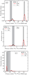 |
Fig. 5. Surface 12C/13C (panel a), 12C/14N (panel b), and 14N/16O (panel c) posterior density distributions of the primary star in the CHeB stage for the full sample as described in Sect. 3.2. In particular, we show the histogram (black lines) and the kernel density estimation with a Gaussian kernel (KDE, red lines). The dashed line and grey area represent the observed values of KIC4937011 and their 1σ errors (also Table 1). As explained in Appendix A, we take the age that gives the highest likelihood as the reference time for the CHeB of each MC simulation. |
To explain the peak at ^12C/^13C ≈ 90, we need a star that contains material in the surface that has not been contaminated by the product of the hydrogen-burning core. This value is not typically observed in CHeB stars because the first dredge-up has already taken place. As explained in Sect. 4.1.1, the CEE phase begins when the binary systems are formed by a red giant primary star and an MS companion. A first dredge-up is forced in HG and RGB stars that undergo a CEE phase, but not for MS stars (Sect. 3.1). In addition, MS stars are assumed to have negligible contamination from companion material because all such material is ejected from the system soon after the CEE phase. We therefore obtain that 69.51% of the full sample of MC simulations (i.e. 45 339 out of 65 225 simulations) after the CEE phase are close binaries formed by a HeWD star and an MS star with M < 0.88 M⊙10 that has not been contaminated by the primary star. These close-binary systems start a stable RLOF from the MS star onto the HeWD star, which eventually formes a single low-mass RGB-like star that later becomes a low-mass CHeB star with a high ^12C/^13C. This formation channel explains the wide distribution of helium-core mass, radius, luminosity, and effective temperature although the distribution in chemistry is narrow; the envelope comes from the MS star and therefore depends more on the chosen initial composition than on internal mixing, atomic diffusion, or overshooting. We highlight that the initial chemical composition of all these MC simulations was taken from Grevesse & Anders (1989) and was therefore fixed for a fixed metallicity (this explains these narrow bins).
The properties of this formation channel agree well with the literature because binary systems formed by a HeWD star and a low-mass MS star are thought to be progenitors of low-mass RGB stars and of hot subdwarfs, depending on the initial properties of the binary system (Hurley et al. 2002; Shen et al. 2009; Clausen & Wade 2011; Pyrzas et al. 2012; Nelemans et al. 2016; Zhang et al. 2017; Rui & Fuller 2024).
4.2. Analysis of a more observationally motivated subsample
In Sect. 4.1.3 we explained that an interaction between a HeWD and a low-mass MS star can produce a low-mass CHeB star with the same mass and age as KIC4937011, but with a higher 12C/14N. In this section we exclude from the analysis all the MC simulations that predict stars that are much brighter and carbon-enriched than observations suggest, which yields more credible formation channels. Based on Figures 4 and 5, we decided to exclude stars with a luminosity and 12C/14N higher than 100 L⊙ and 2.5 because these thresholds differ by at least 5.5σ from the observed values11. The subsample consists of 13.67% of our full sample of MC simulations (i.e. 8917 out of 65 225 simulations) and therefore is a non-negligible part of the full sample, and we have a sufficiently high number of MC simulations to calculate statistics12. In Fig. 6 the corner plot showing the age and primary mass density distributions for the subsample (see also Table 3) is compared with the observed values for KIC4937011 (red lines). Our modelling tends towards higher ages than the full sample, but the observed current age and mass of KIC4937011 are still correctly fitted within the errors.
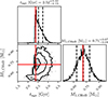 |
Fig. 6. Corner plot showing the age and primary mass density distributions at the CHeB stage for the subsample described in Sect. 4.2. The contours refer to 1, 2, and3 σ. In red we plot the observed values for KIC4937011 (Table 3). As explained in Appendix A, we take as the age that gives the highest likelihood the reference time for the CHeB of each MC simulation. |
4.2.1. New posterior density distributions
We show in Figs. 7, 8 and 9 the estimated posterior density distributions for the subsample (see also Table 3). The anti-correlation between αce ⋅ λce and log P0 still holds, and both distributions have similar 99.7% credible intervals and medians as the full sample (see Fig. 7, Tables 1, 3). The same conclusion holds for the 99.7% credible interval of qZAMS, but not for its median value. This density distribution in the subsample is skewed towards lower values of qZAMS than the full sample (see Tables 1, 3). The density distribution of M1, ZAMS is also skewed towards lower values in the subsample than in the full sample, and it has narrower credible intervals than the full sample (see Tables 1, 3). However, the M1, ZAMS distribution in the subsample is still consistent within the errors with the observed average mass of RGB stars in NGC6819, suggesting a fast evolution after the CE phase. We highlight that the qZAMS posterior distribution is also in the subsample very close to the lower limit we placed on the prior, suggesting the same conclusions as we drew in Sect. 4.1. Finally, as discussed in Sect. 4.1, the high αce ⋅ λce values observed in the subsample can be interpreted as an indication that the recombination energy, dust formation, and nuclear burning affect the CE ejection process.
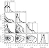 |
Fig. 7. Corner plot showing the posterior density distributions of the subsample described in Sect. 4.2. The contours refer to 1, 2, and 3σ. |
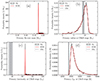 |
Fig. 8. Same as Figure 4, but for the subsample described in Sect. 4.2 (see also Table 3). Effective temperatures above 8000 K are not included in the figure for clarity. As explained in Appendix A, we take the age that gives the highest likelihood as the reference time for the CHeB of each MC simulation. |
The posterior density distributions of helium-core mass, radius, luminosity, and effective temperature are different in the subsample than in the full sample, they have narrower 99.7% credible intervals, and they are more compatible with the observations (see Fig. 8, Tables 1, 3). The helium-core mass distribution is consistent with the theoretical distribution expected for RC stars (Girardi 2016), and it is consistent with the asteroseismic observations of KIC4937011 (Handberg et al. 2017). The radius, luminosity, and effective temperature distributions are a different case because they tend to be systematically skewed towards higher values (see Sect. 4.1.2) than observations and modern evolutionary models (which are more compatible with observations; see Figure 1). Even though the median radius is consistent with the observations within the errors, the median luminosity and effective temperature differ by at least 7σ from the observed values. However, these systematic effects do not limit our inference in the formation channel because they were not used in the likelihood (Appendix A). They were not used to distinguish between models. We therefore decided not to rely on effective temperature, luminosity, and radius to perform a best fit to the observed values in KIC4937011.
For the surface chemical composition distributions (Figure 9 and Table 3), the 12C/13C and 12C/14N posterior distributions are consistent within the errors with the observed values. The 14N/16O posterior distribution tends towards higher values than observations, but with a median of the distribution that differs by just about 1.2σ from the observed value.
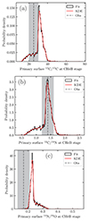 |
Fig. 9. Primary star 12C/13C, 12C/14N and 14N/16O density distributions at the CHeB stage for the subsample described in Sect. 4.2. In particular, we show the histogram (black lines) and the kernel density estimation with a Gaussian kernel (red lines). The dashed line and grey area represent the observed values of KIC4937011 and their 1σ errors (see also Table 1). As explained in Appendix A, we take the age that gives the highest likelihood as the reference time for the CHeB of each MC simulation. |
4.2.2. Most credible formation channel for KIC4937011
In Sect. 4.1.3 we discussed the dichotomy visible in the 12C/14N distribution of the full sample and that the interaction between a HeWD star and an MS star is the main cause of the narrow peak at high 12C/14N. Even in the subsample (that has the lowest values of the 12C/14N distribution) nearly all the MC simulations (99.92% of the subsample, i.e. 8910 out of 8917 simulations) share a similar formation scenario (Fig. 10). As explained in Sect. 3.2 and visible in Fig. 10, we started from two ZAMS stars in a circular orbit. When we consider the 99.7% credible intervals of Table 3, the mass of the primary star lies between 1.46 M⊙ and 1.71 M⊙, the mass of the companion is below 0.71 M⊙, and the orbital period is between 1.15 days and 251 days. A close binary like this starts a RLOF when the primary enters the RGB phase or the HG phase. All these MC simulations predict an unstable RLOF, and thus, a CEE phase arises. The post-CEE phase result is very different from Sect. 4.1.3 because there is no HeWD with a companion MS star. Instead, there is a RGB-like star with an evolved helium core between 0.16 M⊙ and 0.40 M⊙ (99.7% credible intervals; see Figure 10) and a smaller envelope than before the CEE phase (the 99.7% credible interval for the mass of the star is between 0.52 M⊙ and 0.96 M⊙ after the CEE phase; see Figure 10). Simultaneously, there is a median ejection from the system of ≈1.1 M⊙, and the merger of the companion with the helium core of the primary star. During the CEE phase, dynamical mixing effects act owing to the spiral-in process and completely mix the envelope with material from the evolved primary star. After the CEE phase, the RGB-like star has an envelope with the low 12C/14N value we observe today. Finally, this star reaches the CHeB stage after helium flashes as if it were a single star with a mass of ≈0.71 M⊙, consistently with observations. Therefore, this formation channel naturally predicts the low 12C/14N value compatible with RC star of ≈1.6 M⊙ (Sect. 2). Moreover, the R1, CHeB, L1, CHeB, and Teff posterior distributions we found after all these binary interactions are compatible with a ≈0.7 M⊙ CHeB star that evolves in isolation, indicating that our findings are self-consistent within the BINARY_C V2.2.3 framework.
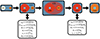 |
Fig. 10. Cartoon showing the most credible formation scenario for KIC4937011. Medians and their 99.7% credible intervals just before and after the CE are also shown. |
However, the high lithium abundance we observe today in KIC4937011 is difficult to explain with this formation channel. Insights into this conundrum may be gleaned from studies of red novae, which are thought to be the direct product of a CEE phase with a merger (Tylenda & Soker 2006; Pastorello et al. 2019). Some of these red novae are rich in lithium (Kamiński et al. 2023), suggesting the involvement of mechanisms capable of synthesizing and mixing lithium during the CEE phase.
Between the post-CEE phase and the CHeB stage, the star evolves in isolation for nearly 150 Myr (maximum a posteriori probability estimate, corresponding to stars with a helium-core mass of about 0.18 M⊙), which is very short compared to the cluster age. We confirmed whether this time and this formation channel are compatible with more advanced evolutionary codes of single stellar evolution. Using the MESA V11701 (Modules for Experiments in Stellar Astrophysics; Paxton et al. 2011, 2019) tool, we tested the pre-CEE and post-CEE phase conditions. We adopted as the reference solar mixture that from Asplund et al. (2009), and high- and low-temperature radiative opacity tables were computed for the solar specific metal mixture. The envelope convection was described by the mixing-length theory Cox & Giuli (1968); the corresponding αMLT parameter, the same for all the models, was derived from the solar calibration with the same physics. Below the convective envelope, we added a diffusive undershooting (Herwig 2000) with a size parameter f = 0.02 (see Khan et al. 2018). Additional mixing over the convective core limit during the CHeB phase was treated following the formalism by Bossini et al. (2017). For the pre-CEE phase, we adopted a 1.60 M⊙ star with Z = 0.022 and Y = 0.28 until it achieved a 0.18 M⊙ helium-core mass in the RGB phase, which took nearly 2.33 Gyr. For the post-CEE phase, we used models with masses between 0.65 M⊙ and 0.80 M⊙ (i.e. a mass range compatible with the 68% credible interval of M1, CHeB in Table 3), and Z = 0.022, Y = 0.28. We did not include any mass loss in these MESA models. It took about 500 Myr for a 0.65 M⊙ star from the RGB phase with a helium-core mass of 0.18 M⊙ to the CHeB stage, and about 370 Myr for a 0.80 M⊙ star. This means that in MESA models, this formation channel would take at least 2.70–2.83 Gyr, which differs by about 1.6σ from the observed value. However, when we consider not just a single value of the helium-core mass, but a distribution of values just before the CEE phase, a final age consistent with BINARY_C V2.2.3 is also possible in MESA. For example, it takes 2.48 Gyr for a 1.60 M⊙ star in MESA to achieve a helium-core mass of 0.22 M⊙ and another about 150 Myr for a star between 0.65 M⊙ and 0.80 M⊙ to ignite helium in the core.
An example of BINARY_C V2.2.3 HRD of a primary star with a formation channel like this is shown in Figure 11. This specific simulation begins with a 1.60 M⊙ ZAMS primary star orbiting a 0.25 M⊙ companion in almost 32 days. The CEE begins when the primary star has a helium-core mass of about 0.279 M⊙, and it ends with the ejection of 1.12 M⊙ of material from the system. The post-CEE star begins the CHeB stage at the age of 2.41 Gyr and a mass of 0.70 M⊙.
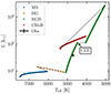 |
Fig. 11. HRD of a primary star in the subsample from the ZAMS to the end of the CHeB stage computed with BINARY_C V2.2.3. The CEE begins when the primary star has a helium-core mass of about 0.279 M⊙ (arrow in the figure), and it ends with the ejection of 1.12 M⊙ of material from the system. The simulation begins with a 1.60 M⊙ ZAMS primary star orbiting a 0.25 M⊙ companion in almost 32 days. The primary star begins the CHeB stage at the age of 2.41 Gyr and a mass of 0.70 M⊙. In black we plot the observed values for KIC4937011 (see also Table 3). |
5. Discussion and conclusions
We focused on the single metal-rich (Z ≈ Z⊙) Li-rich low-mass CHeB star KIC4937011, which is a member of the star cluster NGC 6819 (turn-off mass of ≈1.6 M⊙, i.e. age of ≈2.4 Gyr). The mass of this star is ≈1 M⊙ lower than expected for its age and metallicity. It might therefore be the result of a binary interaction or of the poorly understood mass-loss mechanism along the red giant branch. To infer formation scenarios, we adopted a Bayesian approach using the BINARY_C V2.2.3 code coupled with the dynamic nested-sampling approach contained in the DYNESTY V2.1.1 package. The final conclusions are summarised below.
-
This star is the result of a common-envelope evolution phase in which the companion does not survive. All the MC simulations we considered have one common-envelope phase within the final stage of the CHeB phase of the primary star, and only a negligible fraction of simulations (0.006%) experiences two common-envelope phases.
-
Considering a subsample composed of CHeB primary stars with a luminosity below 100 L⊙ and 12C/14N below 2.5, we find that the highest peak in their helium-core mass density distribution is at 0.4743 M⊙. This is in line with the expectations for RC stars and with the observations of KIC4937011. The 12C/13C and 12C/14N distributions are consistent within the errors with the observations. The 14N/16O posterior distribution tends towards higher values than observations, but with a median of the distribution that differs by just about 1.2σ from the observed value. The effective temperatures, luminosities, and radii distributions are systematically higher than the observations. This is expected, because for these low-mass stars (≈0.7 M⊙), the Pols et al. (1998) evolutionary tracks used in BINARY_C V2.2.3 deviate significantly from more modern evolutionary tracks (Girardi 2016). However, these systematic effects do not limit our inference in the formation channel because they are not used in the likelihood. They are therefore not used to distinguish between models.
-
The most credible formation channel is summarised in Figure 10. We started from two ZAMS stars in a circular orbit. In all the MC simulations we considered, a RLOF begins when the companion is still in the MS phase, but with a primary star that enters the RGB phase or the HG phase. This RLOF is dynamically unstable, and consequently, a CEE phase arises. During this CEE phase, dynamical effects induce a mixing of the envelope of the primary star with the MS companion, forming the chemical pattern we observe today. The final effect of this CEE phase is a median ejection of ≈1.1 M⊙ of material from the system and a simultaneous merger of the companion with the helium-core of the primary star. The post-CEE phase product is an RGB-like star of ≈0.71 M⊙ with an evolved He core. Finally, the star reaches the CHeB stage after helium flashes as if it were a single star. This formation channel is consistent with MESA models of single-star evolution before and after the CEE phase when systematic effects are taken into account.
It is worth mentioning that the same formation channel could form sdB star or metal-rich RR Lyrae (Bobrick et al. 2024), because the effective temperatures in a non-negligible fraction of low-mass CHeB stars reach about 27 000 K. This means that this channel potentially provides another piece of the puzzle in the sequence between RC and sdB stars, or other stripped stars.
We will analyse other very-low mass CHeB stars in open clusters with the same technique because a better statistics of these objects is necessary to verify the formation channel as a universal feature. Furthermore, synthetic populations of Kepler stars provide valuable insights into the overall probability of this evolutionary scenario (Mazzi et al., in prep.). We will also improve the posterior distributions by using detailed evolutionary models within the likelihood in order to compute λce and reduce systematic effects. An analysis of the activity-sensitive He I 10 830 Å absorption triplet would also be interesting in order to better study the current mass loss in KIC4937011 and in order to place this star in the wider context of the Li-rich RC stars (Sneden et al. 2022).
Data availability
The MC simulations underlying this article are shared via the Zenodo link https://zenodo.org/doi/10.5281/zenodo.13712871.
These uncertainties are estimates of the random and systematic effects (due to model physics differences and metal content), respectively.
We did not add the two uncertainties in quadrature because the direct addition is an upper limit of the true uncertainty (Schwarz inequality), which does not depend on any possible correlation between the two.
The renormalised unit weight error (RUWE) is the square root of the normalised chi-square of the astrometric fit to the along-scan observation. It is expected to be 1.0 for well-behaved solutions of single stars (Gaia Collaboration 2016, 2023).
We use the notation log(x)≡log10(x).
We confirmed that uniform priors for M1, ZAMS lead to the same results. However, these new priors require more CPU time.
This age difference is calculated using BINARY_C V2.2.3 at Z = 0.02 and ηRGB = 0.1.
Formally, this is not the same as the 99.7% credible interval of M2, ZAMS in Table 1, but we checked that the companion star has not changed much since the ZAMS.
The most credible formation channel remains the same for a 12C/14N threshold that is still able to separate the two main chemical peaks. The luminosity threshold is necessary in order to exclude stars that approach the beginning of the EAGB.
We confirmed this by randomly sampling one-third of our full sample. We infer the same results even with a reduced number of MC simulations.
Acknowledgments
We are grateful to Raffaele Pascale and Payel Das for useful discussions. We are also grateful to Rasmus Handberg for sharing the data used in Handberg et al. (2017) with us. We thank the anonymous referee for their helpful comments that improved the quality of the manuscript. This work has made use of data from the European Space Agency (ESA) mission Gaia (https://www.cosmos.esa.int/gaia). MM, AM, KB, JM, MT acknowledge support from the ERC Consolidator Grant funding scheme (project ASTEROCHRONOMETRY, https://www.asterochronometry.eu, G.A. n. 772293). We made use of the Python code CORNER (Foreman-Mackey 2016), and of the Python code code KDEPY (https://zenodo.org/doi/10.5281/zenodo.2392267).
References
- Abate, C., Pols, O. R., Izzard, R. G., Mohamed, S. S., & de Mink, S. E. 2013, A&A, 552, A26 [NASA ADS] [CrossRef] [EDP Sciences] [Google Scholar]
- Abate, C., Pols, O. R., Stancliffe, R. J., et al. 2015, A&A, 581, A62 [NASA ADS] [CrossRef] [EDP Sciences] [Google Scholar]
- Aguilera-Gómez, C., Chanamé, J., Pinsonneault, M. H., & Carlberg, J. K. 2016a, ApJ, 829, 127 [Google Scholar]
- Aguilera-Gómez, C., Chanamé, J., Pinsonneault, M. H., & Carlberg, J. K. 2016b, ApJ, 833, L24 [CrossRef] [Google Scholar]
- Aguilera-Gómez, C., Jones, M. I., & Chanamé, J. 2023, A&A, 670, A73 [NASA ADS] [CrossRef] [EDP Sciences] [Google Scholar]
- Anders, F., Chiappini, C., Rodrigues, T. S., et al. 2016, Astron. Nachr., 337, 926 [NASA ADS] [CrossRef] [Google Scholar]
- Anthony-Twarog, B. J., Deliyannis, C. P., Rich, E., & Twarog, B. A. 2013, ApJ, 767, L19 [NASA ADS] [CrossRef] [Google Scholar]
- Anthony-Twarog, B. J., Deliyannis, C. P., & Twarog, B. A. 2014, AJ, 148, 51 [NASA ADS] [CrossRef] [Google Scholar]
- Ashwell, J. F., Jeffries, R. D., Smalley, B., et al. 2005, MNRAS, 363, L81 [NASA ADS] [Google Scholar]
- Asplund, M., Grevesse, N., Sauval, A. J., & Scott, P. 2009, ARA&A, 47, 481 [NASA ADS] [CrossRef] [Google Scholar]
- Auner, G. 1974, A&AS, 13, 143 [NASA ADS] [Google Scholar]
- Babusiaux, C., Fabricius, C., Khanna, S., et al. 2023, A&A, 674, A32 [NASA ADS] [CrossRef] [EDP Sciences] [Google Scholar]
- Basu, S., Grundahl, F., Stello, D., et al. 2011, ApJ, 729, L10 [Google Scholar]
- Bedin, L. R., Salaris, M., Anderson, J., et al. 2015, MNRAS, 448, 1779 [NASA ADS] [CrossRef] [Google Scholar]
- Belloni, D., Schreiber, M. R., & Zorotovic, M. 2024, A&A, 687, A12 [NASA ADS] [CrossRef] [EDP Sciences] [Google Scholar]
- Bobrick, A., Iorio, G., Belokurov, V., et al. 2024, MNRAS, 527, 12196 [Google Scholar]
- Bossini, D., Miglio, A., Salaris, M., et al. 2017, MNRAS, 469, 4718 [Google Scholar]
- Boubert, D., Erkal, D., Evans, N. W., & Izzard, R. G. 2017a, MNRAS, 469, 2151 [NASA ADS] [CrossRef] [Google Scholar]
- Boubert, D., Fraser, M., Evans, N. W., Green, D. A., & Izzard, R. G. 2017b, A&A, 606, A14 [NASA ADS] [CrossRef] [EDP Sciences] [Google Scholar]
- Bragaglia, A., Carretta, E., Gratton, R. G., et al. 2001, AJ, 121, 327 [NASA ADS] [CrossRef] [Google Scholar]
- Brewer, L. N., Sandquist, E. L., Mathieu, R. D., et al. 2016, AJ, 151, 66 [NASA ADS] [CrossRef] [Google Scholar]
- Brogaard, K., Jessen-Hansen, J., Handberg, R., et al. 2016, Astron. Nachr., 337, 793 [NASA ADS] [CrossRef] [Google Scholar]
- Brogaard, K., Christiansen, S. M., Grundahl, F., et al. 2018, MNRAS, 481, 5062 [Google Scholar]
- Brogaard, K., Arentoft, T., Jessen-Hansen, J., & Miglio, A. 2021, MNRAS, 507, 496 [NASA ADS] [CrossRef] [Google Scholar]
- Burkhead, M. S. 1971, AJ, 76, 251 [NASA ADS] [CrossRef] [Google Scholar]
- Cameron, A. G. W., & Fowler, W. A. 1971, ApJ, 164, 111 [NASA ADS] [CrossRef] [Google Scholar]
- Carlberg, J. K., Smith, V. V., Cunha, K., et al. 2015, ApJ, 802, 7 [NASA ADS] [CrossRef] [Google Scholar]
- Casagrande, L., Aguirre, V. S., & Serenelli, A. M. 2016, IAU Focus Meeting, 29B, 680 [Google Scholar]
- Chabrier, G. 2003, PASP, 115, 763 [Google Scholar]
- Chamandy, L., Blackman, E. G., Frank, A., et al. 2019, MNRAS, 490, 3727 [NASA ADS] [CrossRef] [Google Scholar]
- Chiappini, C., Anders, F., Rodrigues, T. S., et al. 2015, A&A, 576, L12 [NASA ADS] [CrossRef] [EDP Sciences] [Google Scholar]
- Chieffi, A., & Limongi, M. 2004, ApJ, 608, 405 [NASA ADS] [CrossRef] [Google Scholar]
- Claeys, J. S. W., Pols, O. R., Izzard, R. G., Vink, J., & Verbunt, F. W. M. 2014, A&A, 563, A83 [NASA ADS] [CrossRef] [EDP Sciences] [Google Scholar]
- Clausen, D., & Wade, R. A. 2011, ApJ, 733, L42 [NASA ADS] [CrossRef] [Google Scholar]
- Cox, J. P., & Giuli, R. T. 1968, Principles of Stellar Structure (New York: Gordon and Breach) [Google Scholar]
- Davis, P. J., Kolb, U., & Knigge, C. 2012, MNRAS, 419, 287 [CrossRef] [Google Scholar]
- de Kool, M. 1990, ApJ, 358, 189 [Google Scholar]
- De Marco, O., & Izzard, R. G. 2017, PASA, 34, e001 [Google Scholar]
- De Marco, O., Passy, J.-C., Moe, M., et al. 2011, MNRAS, 411, 2277 [CrossRef] [Google Scholar]
- de Mink, S. E., Langer, N., Izzard, R. G., Sana, H., & de Koter, A. 2013, ApJ, 764, 166 [Google Scholar]
- De Ridder, J., Barban, C., Baudin, F., et al. 2009, Nature, 459, 398 [Google Scholar]
- Denissenkov, P. A. 2010, ApJ, 723, 563 [NASA ADS] [CrossRef] [Google Scholar]
- Denissenkov, P. A., & Herwig, F. 2004, ApJ, 612, 1081 [NASA ADS] [CrossRef] [Google Scholar]
- Dewi, J. D. M., & Tauris, T. M. 2000, A&A, 360, 1043 [NASA ADS] [Google Scholar]
- Dewi, J. D. M., & Tauris, T. M. 2001, ASP Conf. Ser., 229, 255 [Google Scholar]
- Foreman-Mackey, D. 2016, J. Open Source Softw., 1, 24 [Google Scholar]
- Foreman-Mackey, D., Hogg, D. W., Lang, D., & Goodman, J. 2013, PASP, 125, 306 [Google Scholar]
- Gaia Collaboration (Prusti, T., et al.) 2016, A&A, 595, A1 [NASA ADS] [CrossRef] [EDP Sciences] [Google Scholar]
- Gaia Collaboration (Vallenari, A., et al.) 2023, A&A, 674, A1 [NASA ADS] [CrossRef] [EDP Sciences] [Google Scholar]
- García, R. A., & Ballot, J. 2019, Liv. Rev. Sol. Phys., 16, 4 [Google Scholar]
- Girardi, L. 2016, ARA&A, 54, 95 [Google Scholar]
- Grevesse, N., & Anders, E. 1989, AIP Conf. Ser., 183, 1 [NASA ADS] [CrossRef] [Google Scholar]
- Grisoni, V., Chiappini, C., Miglio, A., et al. 2024, A&A, 683, A111 [NASA ADS] [CrossRef] [EDP Sciences] [Google Scholar]
- Guandalini, R., Palmerini, S., Busso, M., & Uttenthaler, S. 2009, PASA, 26, 168 [NASA ADS] [Google Scholar]
- Halbwachs, J.-L., Pourbaix, D., Arenou, F., et al. 2023, A&A, 674, A9 [NASA ADS] [CrossRef] [EDP Sciences] [Google Scholar]
- Han, Z., Podsiadlowski, P., & Eggleton, P. P. 1994, MNRAS, 270, 121 [NASA ADS] [CrossRef] [Google Scholar]
- Handberg, R., Brogaard, K., Miglio, A., et al. 2017, MNRAS, 472, 979 [CrossRef] [Google Scholar]
- Hekker, S., & Johnson, J. A. 2019, MNRAS, 487, 4343 [NASA ADS] [CrossRef] [Google Scholar]
- Hekker, S., Elsworth, Y., De Ridder, J., et al. 2011, A&A, 525, A131 [NASA ADS] [CrossRef] [EDP Sciences] [Google Scholar]
- Hendriks, D. D., & Izzard, R. G. 2023, J. Open Source Softw., 8, 4642 [NASA ADS] [CrossRef] [Google Scholar]
- Herwig, F. 2000, A&A, 360, 952 [NASA ADS] [Google Scholar]
- Hole, K. T., Geller, A. M., Mathieu, R. D., et al. 2009, AJ, 138, 159 [CrossRef] [Google Scholar]
- Huber, D., Bedding, T. R., Stello, D., et al. 2011, ApJ, 743, 143 [Google Scholar]
- Hurley, J. R., Pols, O. R., & Tout, C. A. 2000, MNRAS, 315, 543 [Google Scholar]
- Hurley, J. R., Tout, C. A., & Pols, O. R. 2002, MNRAS, 329, 897 [Google Scholar]
- Iaconi, R., & De Marco, O. 2019, MNRAS, 490, 2550 [Google Scholar]
- Ivanova, N., & Chaichenets, S. 2011, ApJ, 731, L36 [NASA ADS] [CrossRef] [Google Scholar]
- Ivanova, N., Justham, S., Chen, X., et al. 2013, A&ARv, 21, 59 [Google Scholar]
- Izzard, R. G., & Jermyn, A. S. 2023, MNRAS, 521, 35 [NASA ADS] [CrossRef] [Google Scholar]
- Izzard, R. G., Tout, C. A., Karakas, A. I., & Pols, O. R. 2004, MNRAS, 350, 407 [CrossRef] [Google Scholar]
- Izzard, R. G., Dray, L. M., Karakas, A. I., Lugaro, M., & Tout, C. A. 2006, A&A, 460, 565 [NASA ADS] [CrossRef] [EDP Sciences] [Google Scholar]
- Izzard, R. G., Glebbeek, E., Stancliffe, R. J., & Pols, O. R. 2009, A&A, 508, 1359 [NASA ADS] [CrossRef] [EDP Sciences] [Google Scholar]
- Izzard, R. G., Preece, H., Jofre, P., et al. 2018, MNRAS, 473, 2984 [NASA ADS] [CrossRef] [Google Scholar]
- Jeffries, M. W., Jr., Sandquist, E. L., Mathieu, R. D., et al. 2013, AJ, 146, 58 [NASA ADS] [CrossRef] [Google Scholar]
- José, J., & Hernanz, M. 1998, ApJ, 494, 680 [Google Scholar]
- Kalirai, J. S., Richer, H. B., Fahlman, G. G., et al. 2001, AJ, 122, 266 [NASA ADS] [CrossRef] [Google Scholar]
- Kallinger, T. 2019, arXiv e-prints [arXiv:1906.09428] [Google Scholar]
- Kamiński, T., Schmidt, M., Hajduk, M., et al. 2023, A&A, 672, A196 [NASA ADS] [CrossRef] [EDP Sciences] [Google Scholar]
- Karakas, A. I., Lattanzio, J. C., & Pols, O. R. 2002, PASA, 19, 515 [NASA ADS] [CrossRef] [Google Scholar]
- Khan, S., Hall, O. J., Miglio, A., et al. 2018, ApJ, 859, 156 [NASA ADS] [CrossRef] [Google Scholar]
- Kim, W.-T. 2010, ApJ, 725, 1069 [NASA ADS] [CrossRef] [Google Scholar]
- Kudritzki, R. P., & Reimers, D. 1978, A&A, 70, 227 [Google Scholar]
- Lee-Brown, D. B., Anthony-Twarog, B. J., Deliyannis, C. P., Rich, E., & Twarog, B. A. 2015, AJ, 149, 121 [NASA ADS] [CrossRef] [Google Scholar]
- Li, Y., Bedding, T. R., Murphy, S. J., et al. 2022, Nat. Astron., 6, 673 [NASA ADS] [CrossRef] [Google Scholar]
- Lindoff, U. 1972, A&AS, 7, 497 [NASA ADS] [Google Scholar]
- Livio, M., & Soker, N. 1988, ApJ, 329, 764 [Google Scholar]
- MacLeod, M., & Ramirez-Ruiz, E. 2015, ApJ, 803, 41 [Google Scholar]
- Mallick, A., Reddy, B. E., & Muthumariappan, C. 2022, MNRAS, 511, 3741 [NASA ADS] [CrossRef] [Google Scholar]
- Martig, M., Rix, H.-W., Silva Aguirre, V., et al. 2015, MNRAS, 451, 2230 [NASA ADS] [CrossRef] [Google Scholar]
- Matteuzzi, M., Montalbán, J., Miglio, A., et al. 2023, A&A, 671, A53 [NASA ADS] [CrossRef] [EDP Sciences] [Google Scholar]
- Miglio, A., Chiappini, C., Morel, T., et al. 2013, MNRAS, 429, 423 [Google Scholar]
- Miglio, A., Chiappini, C., Mackereth, J. T., et al. 2021, A&A, 645, A85 [NASA ADS] [CrossRef] [EDP Sciences] [Google Scholar]
- Montalbán, J., Mackereth, J. T., Miglio, A., et al. 2021, Nat. Astron., 5, 640 [Google Scholar]
- Mosser, B., Benomar, O., Belkacem, K., et al. 2014, A&A, 572, L5 [NASA ADS] [CrossRef] [EDP Sciences] [Google Scholar]
- Nelemans, G., Siess, L., Repetto, S., Toonen, S., & Phinney, E. S. 2016, ApJ, 817, 69 [NASA ADS] [CrossRef] [Google Scholar]
- Ohlmann, S. T., Röpke, F. K., Pakmor, R., & Springel, V. 2016, ApJ, 816, L9 [Google Scholar]
- Paczyński, B. 1976, Symp. Int. Astron. Union, 73, 75 [CrossRef] [Google Scholar]
- Pastorello, A., Mason, E., Taubenberger, S., et al. 2019, A&A, 630, A75 [NASA ADS] [CrossRef] [EDP Sciences] [Google Scholar]
- Paxton, B., Bildsten, L., Dotter, A., et al. 2011, ApJS, 192, 3 [Google Scholar]
- Paxton, B., Smolec, R., Schwab, J., et al. 2019, ApJS, 243, 10 [Google Scholar]
- Pinsonneault, M. H., Elsworth, Y. P., Tayar, J., et al. 2018, ApJS, 239, 32 [Google Scholar]
- Podsiadlowski, P., Rappaport, S., & Han, Z. 2003, MNRAS, 341, 385 [NASA ADS] [CrossRef] [Google Scholar]
- Politano, M. 2004, ApJ, 604, 817 [NASA ADS] [CrossRef] [Google Scholar]
- Pols, O. R., Schröder, K.-P., Hurley, J. R., Tout, C. A., & Eggleton, P. P. 1998, MNRAS, 298, 525 [Google Scholar]
- Pyrzas, S., Gänsicke, B. T., Brady, S., et al. 2012, MNRAS, 419, 817 [NASA ADS] [CrossRef] [Google Scholar]
- Rebull, L. M., Carlberg, J. K., Gibbs, J. C., et al. 2015, AJ, 150, 123 [NASA ADS] [CrossRef] [Google Scholar]
- Reichardt, T. A., De Marco, O., Iaconi, R., Tout, C. A., & Price, D. J. 2019, MNRAS, 484, 631 [NASA ADS] [CrossRef] [Google Scholar]
- Reimers, D. 1975, MSRSL, 8, 369 [NASA ADS] [Google Scholar]
- Röpke, F. K., & De Marco, O. 2023, Liv. Rev. Comput. Astrophys., 9, 2 [CrossRef] [Google Scholar]
- Rosvick, J. M., & Vandenberg, D. A. 1998, AJ, 115, 1516 [NASA ADS] [CrossRef] [Google Scholar]
- Rui, N. Z., & Fuller, J. 2024, Open J. Astrophys., 7, 81 [NASA ADS] [CrossRef] [Google Scholar]
- Rybizki, J., Green, G. M., Rix, H.-W., et al. 2022, MNRAS, 510, 2597 [NASA ADS] [CrossRef] [Google Scholar]
- Salaris, M., Pietrinferni, A., Piersimoni, A. M., & Cassisi, S. 2015, A&A, 583, A87 [NASA ADS] [CrossRef] [EDP Sciences] [Google Scholar]
- Sand, C., Ohlmann, S. T., Schneider, F. R. N., Pakmor, R., & Röpke, F. K. 2020, A&A, 644, A60 [NASA ADS] [CrossRef] [EDP Sciences] [Google Scholar]
- Schneider, F. R. N., Izzard, R. G., de Mink, S. E., et al. 2014, ApJ, 780, 117 [Google Scholar]
- Shen, K. J., Idan, I., & Bildsten, L. 2009, ApJ, 705, 693 [NASA ADS] [CrossRef] [Google Scholar]
- Shima, E., Matsuda, T., Takeda, H., & Sawada, K. 1985, MNRAS, 217, 367 [NASA ADS] [Google Scholar]
- Siess, L., Izzard, R. G., Davis, P. J., & Deschamps, R. 2013, A&A, 550, A100 [NASA ADS] [CrossRef] [EDP Sciences] [Google Scholar]
- Silva Aguirre, V., Bojsen-Hansen, M., Slumstrup, D., et al. 2018, MNRAS, 475, 5487 [NASA ADS] [Google Scholar]
- Slumstrup, D., Grundahl, F., Silva Aguirre, V., & Brogaard, K. 2019, A&A, 622, A111 [NASA ADS] [CrossRef] [EDP Sciences] [Google Scholar]
- Sneden, C., Afşar, M., Bozkurt, Z., et al. 2022, ApJ, 940, 12 [NASA ADS] [CrossRef] [Google Scholar]
- Speagle, J. S. 2020, MNRAS, 493, 3132 [Google Scholar]
- Stancliffe, R. J., Glebbeek, E., Izzard, R. G., & Pols, O. R. 2007, A&A, 464, L57 [NASA ADS] [CrossRef] [EDP Sciences] [Google Scholar]
- Stello, D., Huber, D., Bedding, T. R., et al. 2013, ApJ, 765, L41 [CrossRef] [Google Scholar]
- Taam, R. E., & Sandquist, E. L. 2000, ARA&A, 38, 113 [NASA ADS] [CrossRef] [Google Scholar]
- Tayar, J., Carlberg, J. K., Aguilera-Gómez, C., & Sayeed, M. 2023, AJ, 166, 60 [NASA ADS] [CrossRef] [Google Scholar]
- Tylenda, R., & Soker, N. 2006, A&A, 451, 223 [NASA ADS] [CrossRef] [EDP Sciences] [Google Scholar]
- van den Heuvel, E. P. J. 1976, Symp. Int. Astron. Union, 73, 35 [NASA ADS] [CrossRef] [Google Scholar]
- Wang, C., Jia, K., & Li, X.-D. 2016, Res. Astron. Astrophys., 16, 126 [NASA ADS] [Google Scholar]
- Webbink, R. F. 1984, ApJ, 277, 355 [NASA ADS] [CrossRef] [Google Scholar]
- Webbink, R. F. 2008, Astrophys. Space Sci. Lib., 352, 233 [NASA ADS] [CrossRef] [Google Scholar]
- Wong, T.-W., Valsecchi, F., Ansari, A., et al. 2014, ApJ, 790, 119 [NASA ADS] [CrossRef] [Google Scholar]
- Woosley, S. E., & Weaver, T. A. 1995, ApJS, 101, 181 [Google Scholar]
- Xu, X.-J., & Li, X.-D. 2010a, ApJ, 716, 114 [Google Scholar]
- Xu, X.-J., & Li, X.-D. 2010b, ApJ, 722, 1985 [NASA ADS] [CrossRef] [Google Scholar]
- Yang, S.-C., Sarajedini, A., Deliyannis, C. P., et al. 2013, ApJ, 762, 3 [NASA ADS] [CrossRef] [Google Scholar]
- Yates, R. M., Hendriks, D., Vijayan, A. P., et al. 2024, MNRAS, 527, 6292 [Google Scholar]
- Yu, J., Huber, D., Bedding, T. R., et al. 2018, ApJS, 236, 42 [NASA ADS] [CrossRef] [Google Scholar]
- Zamora, O., Abia, C., Plez, B., & Domınguez, I. 2006, Mem. Soc. Astron. It., 77, 973 [NASA ADS] [Google Scholar]
- Zhang, X., Hall, P. D., Jeffery, C. S., & Bi, S. 2017, ApJ, 835, 242 [NASA ADS] [CrossRef] [Google Scholar]
- Zhang, X., Jeffery, C. S., Li, Y., & Bi, S. 2020, ApJ, 889, 33 [NASA ADS] [CrossRef] [Google Scholar]
Appendix A: Likelihood and prior functions
As discussed in Section 3.2, we calculate the likelihood function given the current evolutionary phase (CHeB stage), mass (M1, obs ± σ1, obs = 0.71 ± 0.08 M⊙) and age (tage, obs ± σage, obs = 2.38 ± 0.27 Gyr) of KIC4937011. We employ the multivariate normal likelihood
![Mathematical equation: $$ \begin{aligned} \mathcal{N} (\mathbf{x} | \boldsymbol{\mu },\boldsymbol{C}) = \max _{ \boldsymbol{t_{\mathrm{age, \, mod}}}} \frac{1}{2 \pi \sqrt{| \mathbf{C}|} } \exp { \left[ - \frac{1}{2} \left( \mathbf{x} - \boldsymbol{\mu } \right)^T \boldsymbol{C}^{-1} \left( \mathbf{x} - \boldsymbol{\mu } \right) \right] } \end{aligned} $$](/articles/aa/full_html/2024/11/aa51092-24/aa51092-24-eq7.gif) (A.1)
(A.1)
with x = [tage, obs; M1, obs], μ = [tage, mod; M1, mod], and C = diag(σage, obs2; σ1, obs2). It is not possible to univocally associate an age with the CHeB stage, because several ages (tage, mod and the corresponding mass M1, mod are not scalars) correspond to the same evolutionary phase. Therefore, for each evolutionary track we calculate the likelihood corresponding to all ages in the same evolutionary phase and we keep the age that leads to the highest likelihood as a characteristic age to associate at the CHeB stage of that evolutionary track.
In Table A.1 the intervals of the priors. From a comparison with Table 1 and 3 we can note that three free parameters are well constrained within the intervals. This suggests that it is not necessary to widen these ranges because we explore the free-parameters space thoroughly. However, qZAMS has a lower bound of the posterior distribution that touches our chosen prior (see discussion in Section 4.1 and 4.2).
Intervals of the priors used in Section 3.2.
We also explore the posterior distributions using the same priors and likelihood, but with the Markov Chain Monte Carlo algorithm (MCMC) present in the EMCEE Python package (Foreman-Mackey et al. 2013). We obtain results consistent with Section 4.
All Tables
Critical mass ratio qcrit for stable RLOF for different types of donor stars in the case of a non-degenerate and a degenerate accretor.
All Figures
|
Fig. 1. HRD of NGC 6819 showing RC and RGB member stars. Except for standard single stars, some are members of binary systems, some are overmassive stars, and one star (KIC4937011) is undermassive. The solid lines show evolutionary tracks from the RGB phase until the first thermal pulse in the AGB phase for a 1.60 M⊙ and a 2.50 M⊙ star with solar metallicity, and the dotted line represents a 0.70 M⊙ star with solar metallicity from the beginning of the CHeB stage until the first thermal pulse in the AGB phase. KIC4937011 is dimmer and cooler than other member stars at the same evolutionary stage, and it would be compatible with a 1.60 M⊙ RGB star if we had no information about its evolutionary state and mass. For a full description of the models used in the figure, see Handberg et al. (2017). |
| In the text | |
|
Fig. 2. Corner plot showing the age and primary mass density distributions at the CHeB stage for the full sample as described in Sect. 3.2. The contours refer to the 1, 2, and 3σ credible regions. The observed values for KIC4937011 are plotted in red (see also Table 1). We see that our modelling correctly fits, within errors, the observed current age and mass of KIC4937011. As explained in Appendix A, we take as the reference time for the CHeB of each MC simulation the age that gives the highest likelihood. |
| In the text | |
|
Fig. 3. Corner plot showing the posterior density distributions of the MC simulations described in Sect. 3.2. The contours refer to 1, 2, and 3 σ. |
| In the text | |
|
Fig. 4. Helium-core mass (panel a), radius (panel b), luminosity (panel c), and effective temperature (panel d) posterior density distributions of the primary star during the CHeB stage for the full sample described in Sect. 3.2. We show the histogram (black lines) and the kernel density estimate with a Gaussian kernel (KDE, red lines). The dashed line and the grey area represent the KIC4937011 observations and their 1σ errors (Table 1). Effective temperatures above 8000 K are omitted from the figure for clarity. As explained in Appendix A, we take the age that gives the highest likelihood as the reference time for the CHeB of each MC simulation. |
| In the text | |
|
Fig. 5. Surface 12C/13C (panel a), 12C/14N (panel b), and 14N/16O (panel c) posterior density distributions of the primary star in the CHeB stage for the full sample as described in Sect. 3.2. In particular, we show the histogram (black lines) and the kernel density estimation with a Gaussian kernel (KDE, red lines). The dashed line and grey area represent the observed values of KIC4937011 and their 1σ errors (also Table 1). As explained in Appendix A, we take the age that gives the highest likelihood as the reference time for the CHeB of each MC simulation. |
| In the text | |
|
Fig. 6. Corner plot showing the age and primary mass density distributions at the CHeB stage for the subsample described in Sect. 4.2. The contours refer to 1, 2, and3 σ. In red we plot the observed values for KIC4937011 (Table 3). As explained in Appendix A, we take as the age that gives the highest likelihood the reference time for the CHeB of each MC simulation. |
| In the text | |
|
Fig. 7. Corner plot showing the posterior density distributions of the subsample described in Sect. 4.2. The contours refer to 1, 2, and 3σ. |
| In the text | |
|
Fig. 8. Same as Figure 4, but for the subsample described in Sect. 4.2 (see also Table 3). Effective temperatures above 8000 K are not included in the figure for clarity. As explained in Appendix A, we take the age that gives the highest likelihood as the reference time for the CHeB of each MC simulation. |
| In the text | |
|
Fig. 9. Primary star 12C/13C, 12C/14N and 14N/16O density distributions at the CHeB stage for the subsample described in Sect. 4.2. In particular, we show the histogram (black lines) and the kernel density estimation with a Gaussian kernel (red lines). The dashed line and grey area represent the observed values of KIC4937011 and their 1σ errors (see also Table 1). As explained in Appendix A, we take the age that gives the highest likelihood as the reference time for the CHeB of each MC simulation. |
| In the text | |
|
Fig. 10. Cartoon showing the most credible formation scenario for KIC4937011. Medians and their 99.7% credible intervals just before and after the CE are also shown. |
| In the text | |
|
Fig. 11. HRD of a primary star in the subsample from the ZAMS to the end of the CHeB stage computed with BINARY_C V2.2.3. The CEE begins when the primary star has a helium-core mass of about 0.279 M⊙ (arrow in the figure), and it ends with the ejection of 1.12 M⊙ of material from the system. The simulation begins with a 1.60 M⊙ ZAMS primary star orbiting a 0.25 M⊙ companion in almost 32 days. The primary star begins the CHeB stage at the age of 2.41 Gyr and a mass of 0.70 M⊙. In black we plot the observed values for KIC4937011 (see also Table 3). |
| In the text | |
Current usage metrics show cumulative count of Article Views (full-text article views including HTML views, PDF and ePub downloads, according to the available data) and Abstracts Views on Vision4Press platform.
Data correspond to usage on the plateform after 2015. The current usage metrics is available 48-96 hours after online publication and is updated daily on week days.
Initial download of the metrics may take a while.