| Issue |
A&A
Volume 693, January 2025
|
|
|---|---|---|
| Article Number | A207 | |
| Number of page(s) | 13 | |
| Section | Extragalactic astronomy | |
| DOI | https://doi.org/10.1051/0004-6361/202450813 | |
| Published online | 20 January 2025 | |
The dynamical lineage of isolated, HI-rich ultra-diffuse galaxies
Indian Institute of Science Education and Research, Tirupati 517619, India
⋆ Corresponding authors; nandi.nilanjana154@gmail.com, arunima@iisertirupati.ac.in
Received:
21
May
2024
Accepted:
23
November
2024
Context. Ultra-diffuse galaxies (UDGs) exhibit morphological similarities with other low-luminosity galaxies, indicating a possible evolutionary connection.
Aims. We investigated for the common dynamical characteristics of isolated, HI-rich UDGs with other low-luminosity field galaxies, namely the low surface brightness galaxies (LSBs) and the dwarf irregulars (dIrrs).
Methods. We considered samples of each of the UDGs, LSBs, and the dIrrs. We first obtained scaling relations involving mass and structural parameters for the LSB and the dIrr samples and superposed the UDGs on them. We then carried out a two-sample Anderson-Darling test to analyse whether the UDGs belong to the population of the LSBs or the dIrrs. Thereafter, we constructed distribution function-based stellar-dynamical models of these galaxies to determine their kinematical parameters. We followed up with the Mann-Whitney U-test to determine if our UDG, LSB, and dIrr samples belong to different parent populations so far as kinematics is concerned. Finally, we conducted principal component analyses involving both structural and kinematical parameters to identify the key properties accounting for the variance in the data for the respective galaxy populations.
Results. From the galaxy scaling relation studies, we note that the UDGs and the LSBs constitute statistically different populations. However, for the UDGs and the dIrrs, the null hypotheses of these statistical tests cannot be rejected for the following scaling relations: (i) stellar mass versus atomic hydrogen mass, (ii) stellar mass versus dynamical mass, and (iii) dark matter core density versus core radius. Interestingly, the dynamical models suggest that the UDGs, LSBs, and the dIrrs constitute different galaxy populations, as reflected by their radial-to-vertical velocity dispersion and the rotational velocity-to-total stellar velocity dispersion. Finally, we observe that the total HI and stellar mass mostly regulate the variance in the structural and kinematical data for both the UDGs and the dIrrs, while the ratio of radial-to-vertical velocity dispersion and the total HI mass dominate the variation in the LSBs.
Conclusions. The UDGs and the LSBs represent statistically different galaxy populations with respect to their mass and structural properties. However, the statistical studies do not negate the fact that the structural parameters of the UDGs and the dIrrs follow the same normal distributions. However, the UDGs, LSBs, and the dIrrs constitute very different populations as far as their kinematical parameters are concerned. Finally, we note that the variation in the structural and kinematical data of both the UDGs and the dIrrs is mostly accounted for by their stellar mass and HI mass, whereas for the LSBs, the variance is explained by the ratio of the radial-to-vertical stellar dispersion followed by the HI mass. Thus, we may conclude that the UDGs and dIrrs share a common dynamical lineage.
Key words: galaxies: dwarf / galaxies: evolution / galaxies: formation / galaxies: irregular / galaxies: kinematics and dynamics / galaxies: structure
© The Authors 2025
 Open Access article, published by EDP Sciences, under the terms of the Creative Commons Attribution License (https://creativecommons.org/licenses/by/4.0), which permits unrestricted use, distribution, and reproduction in any medium, provided the original work is properly cited.
This article is published in open access under the Subscribe to Open model. Subscribe to A&A to support open access publication.
1. Introduction
In the last few decades, an increasingly large number of faint galaxies have been detected with the development of observational facilities. These low-luminosity galaxies constitute a significant fraction of the galaxy population in the nearby universe (van Dokkum et al. 2015a,b; Yagi et al. 2016; Román & Trujillo 2017; Shi et al. 2017; Prole et al. 2019; Ikeda et al. 2023). In general, they are gas-rich and dark matter-dominated and hence constitute ideal test beds for galaxy formation and evolution models (Sandage & Binggeli 1984; Impey et al. 1988; Bothun et al. 1997). Ultra-diffuse galaxies (UDGs) constitute a class of low-luminosity galaxies, and some of these galaxies are claimed to be dark matter-deficient by several studies, for example, van Dokkum et al. (2018, 2019), Danieli et al. (2019), Mancera Piña et al. (2022a), and Mancera Piña et al. (2024), and are hence enigmatic. The term ultra-diffuse galaxy, or ‘UDG’, was coined by van Dokkum et al. (2015a), who defined these as galaxies with central g-band surface brightness μg, 0> 24 mag arcsec−2 and effective radii Re > 1.5 kpc. UDGs are, therefore, characterised by very low central surface brightness and relatively large stellar disc scale lengths, given their stellar masses, M*, in the dwarf galaxy regime (M* ≡ 106 − 9 M⊙). UDGs can be found in a range of environments: from clusters and groups to fields, and their structure and kinematics seem to vary significantly with their environment (Martínez-Delgado et al. 2016, Yagi et al. 2016, Janssens et al. 2017, 2019, van der Burg et al. 2017, Román & Trujillo 2017, Müller et al. 2018, Forbes et al. 2019, Prole et al. 2019, Zaritsky et al. 2019, Román et al. 2019, Barbosa et al. 2020).
Recent observational studies have identified morphological and kinematical similarities between UDGs and other low-luminosity galaxies, thus hinting at possible evolutionary links among them. Venhola et al. (2017) found that dwarf low surface brightness galaxies (LSBs) and UDGs in the Fornax cluster share similar structural properties, possibly indicating a common genesis of these galaxy populations. Mancera Piña et al. (2019a) studied the structural properties of a large sample of UDGs distributed at different radii within eight nearby galaxy clusters. Curiously, they observed similarities in the distribution of the axial ratios of the UDGs with those of the late-type dwarfs and dwarf ellipticals (dEs) in the Fornax cluster, thus suggesting a link between UDGs and dwarfs. While studying the kinematic properties of two field dwarf irregular galaxies (dIrrs), Bellazzini et al. (2017) concluded that dIrrs and UDGs lie close to each other in the magnitude-effective radius space. In addition, the isolated UDGs are observed to have a relatively higher gas fraction compared to other gas-rich ‘normal’ galaxies, which is similar to the trend observed in fainter and smaller dIrrs (Lee et al. 2003, Leisman et al. 2017). Based on their size and absolute magnitude distribution, Conselice (2018) concluded that UDGs and dEs in clusters are essentially the same objects. Further, UDGs in the Coma cluster were found to lie in between dEs or dwarf lenticular galaxies (dS0s) and dwarf spheroidal galaxies (dSphs), both in the Faber-Jackson relation as well as the mass-metallicity relation (Chilingarian et al. 2019). This may suggest that UDGs constitute an intermediate evolutionary state between dE0 as well as dS0 and dSphs. Aside from these, by studying the stellar kinematics of KDG64, a large dSph galaxy in the M81 group, Afanasiev et al. (2023) concluded that it is possibly in a transitional stage between a dSph and a UDG. While the formation scenario of UDGs is still debatable, modelling their structure and kinematics may enhance our understanding of their evolutionary link with other low-luminosity galaxies. Despite empirical evidence hinting at an evolutionary connection between UDGs and other low-luminosity galaxies, to our knowledge, a systematic study has not been done so far to investigate the dynamical connection among them.
Our primary aim in this paper is to investigate the dynamical lineage of isolated, HI-rich UDGs and other low-luminosity samples, namely LSBs and dIrrs, and look for a possibly common origin. LSBs are defined as galaxies that have surface brightness lesser than the night sky, their central surface brightness in B-band (μB, 0) being > 23 mag arcsec−2 (Impey & Bothun 1997). Recent studies indicate that LSBs are formed inside dark matter halos with a higher spin parameter (λ> 0.05) (Pérez-Montaño & Cervantes Sodi 2019 and the references therein). Since the dark matter halo and the baryonic component have the same specific angular momentum before the formation of the galactic disc (Efstathiou & Silk 1983; Mo et al. 2010), a higher specific angular momentum results in a lower stellar surface density. Therefore, LSBs can be considered to be the fallouts of the high value of the dark matter spin parameter (Dalcanton et al. 1997; Mo et al. 1998; Boissier et al. 2003; Kim & Lee 2013; Jadhav Y & Banerjee 2019). LSBs include a broad range of galaxies based on mass, size, and morphology. However, the field LSBs, which are also the LSBs used in this study, are primarily disc-dominated late-type galaxies that can be safely classified as non-dwarfs (de Blok et al. 1996, van den Hoek et al. 2000, O’Neil et al. 2004). On the other hand, dIrrs are classified by their irregular morphology with lower intrinsic luminosities, their B-band absolute magnitude MB > −18 (van Zee 2000, 2001; Pokhrel et al. 2020). The formation of dIrrs is attributed to two distinct formation mechanisms: 1) Collapse of primordial gas clouds 2) Tidal torquing or stirring of satellite galaxies by the gravitational potential of the host galaxy (Hunter et al. 2000). Field UDGs are generally considered as LSBs with lower mass but larger radial extent (for example, Martin et al. 2019; Prole et al. 2021; Brook et al. 2021; Zhou et al. 2022); on the other hand, they are often categorised under the same class as the dIrrs, as suggested by their morphological similarities (for example, Bellazzini et al. 2017; Prole et al. 2019). In this paper, we aimed to distinguish among these different classes of galaxies in terms of their structural as well as kinematic properties, choosing suitable samples from the UDG, LSB, and the dIrr populations. We first checked for viable correlations between different pairs of structural parameters for each of the above galaxy populations, and in the case of a correlation, we noted if the different populations obey the same scaling relation. We then constructed the distribution function-based dynamical models of some of the galaxies in the three respective populations, employing the publicly available stellar dynamical code Action-based Galaxy Modelling Architecture (AGAMA) (Vasiliev 2019). Finally, for each galaxy population, we did principal component analyses (PCA) (Bro & Smilde 2014, for reference) considering a set of their structural and kinematic parameters and identified the key physical properties regulating the dynamics of each population.
The paper is organised as follows: In Sect. 2, we introduce galaxy scaling relations, and in Sect. 3, the dynamical models. In Sects. 4, 5, and 6, we present our galaxy samples, the source of input parameters, and our methodologies, respectively. We present results and discussion in Sect. 7, and finally the conclusions in Sect. 8.
2. Galaxy scaling relations
According to the current paradigm of galaxy formation, galactic discs are formed at the centres of slowly rotating dark matter halos, due to cooling and condensation of gas, followed by star formation and feedback. Theoretical models of galaxy formation are constrained by the remarkable regularities exhibited by the observed scaling relations between different pairs of structural and kinematic properties of a galaxy population: the Tully-Fisher relation, the Faber-Jackson relation, the Fall relation, and the Kennicutt-Schmidt relation are some of the well-known scaling relations observed in galaxies (for example, da Costa & Renzini 1997). However, the details of the scaling relations may tend to vary with galaxies of different morphological types, possibly indicating their different evolutionary routes (Roychowdhury et al. 2009; Wyder et al. 2009; Jadhav Y & Banerjee 2019; Romeo et al. 2020, 2023; Narayanan & Banerjee 2022 and the references therein). Compliance of UDGs with the scaling relations obeyed by ordinary disc galaxies has been studied earlier in the literature (for example, Poulain et al. 2022; Benavides et al. 2023; For et al. 2023; Hu et al. 2023 and the references therein). In this context, we note that several studies have shown that the gas-rich UDGs do not follow the baryonic Tully-Fisher relation; they rotate significantly more slowly compared to galaxies with similar baryonic mass. (Mancera Piña et al. 2019b, 2020; Karunakaran et al. 2020; Du et al. 2024). In this work, we looked for feasible scaling relations between a few other pairs of dynamical parameters for our LSB and dIrr samples and checked if the distribution of our sample UDGs is resemblant of the LSB or the dIrr population.
3. Dynamical model
As discussed, the definitions of these galaxy types are based on their optical properties, such as absolute magnitude and surface brightness, which depend on their stellar component. For example, the LSBs and the dIrrs can be easily distinguished in terms of their optical images. On the other hand, UDGs, LSBs, and dIrrs may not be very different as far as their HI parameters are concerned. In this work, we used the observed stellar (radial stellar surface density profile) as well as HI profiles (radial HI surface density profile, HI rotation curve) to constrain the total dynamical model of a galaxy, which involves a self-gravitating stellar disc subjected to the external gravitational potential of a gas disc and a dark matter halo. The underlying assumption is that the HI rotation curve is the same as the stellar one, which is not necessarily the case in general (for example, Leaman et al. 2012, Mancera Piña et al. 2021a, Taibi et al. 2024).
We employed the publicly available stellar dynamical code AGAMA to construct distribution function-based dynamical models for our sample galaxies (Vasiliev 2019). Each of our galaxy models consisted of a self-gravitating stellar disc, characterised by a distribution function (DF), also subjected to the static external potentials of the gas disc and the dark matter halo. According to the strong Jeans’ Theorem, the DF J(x, v|Φ) can be expressed as a function of the actions that depend on the total potential Φ of the system, with x and v being the position and velocity of the stellar disc particles.
In this work, we considered the stellar component of the galaxy to have a quasi-isothermal DF which is expressed as follows:
Here κ and ν represent the epicyclic frequencies in the radial and vertical directions, respectively, with their expressions being
while σr, * and σz, * are the stellar velocity dispersions in the corresponding directions. Jr, Jϕ, and Jz, respectively, correspond to the r, ϕ, and z components of the action of the stellar disc. The actions in the radial and vertical directions are, respectively, Jr = ER/κ and Jz = Ez/ν, ER representing the energy of planar motion and Ez the energy for vertical motion. Jϕ can be represented as  , and the magnitude of the total action J is given by J2 = Jr2 + Jϕ2 + Jz2. Here Φ is the net potential due to the stars, gas, and the dark matter halo and is given by the Poisson equation as follows:
where ρs, ρg, and ρDM are the densities of the stars, gas, and dark matter halo, respectively. In the AGAMA framework, the density profile of a disc distribution is given by:
![$$ \begin{aligned} \rho = \Sigma _0\,\exp \left(-\left[\frac{R}{R_D}\right]^{\frac{1}{n}} - \frac{R_\mathrm{cut} }{R}\right) \times \left\{ \!\!\begin{array}{ll} \delta (z)&h = 0 \\ [1mm] \frac{1}{2h} \exp \left(-\big |\frac{z}{h}\big |\right)&h>0 \\ [1mm] \frac{1}{4|h|}\, \mathrm{sech} ^2\left(\big |\frac{z}{2h}\big |\right)&h < 0 \end{array} \right.\!\!\!\!, \end{aligned} $$](/articles/aa/full_html/2025/01/aa50813-24/aa50813-24-eq5.gif)
where Σ0 and RD denote the central surface brightness and disc scale length, respectively. Here, h is the vertical disc scale height, and Rcut an inner cut-off radius that modifies the inner density distribution of the disc. Sérsic index n is taken to be, respectively, 1 and 0.5 for exponential and sech-squared (roughly) profiles. We assumed that the stellar and the gas components have disc-like and sech-squared radial density profiles, respectively.
For modelling the dark matter halo, we used the spheroidal profile given by the following:
![$$ \begin{aligned} \rho = \rho _0 \left(\frac{r}{R_c}\right)^{-\gamma } \bigg [ 1 + \bigg (\frac{ r}{R_c}\bigg )^\alpha \bigg ]^{\frac{\gamma -\beta }{\alpha }} \times \exp \bigg [-\bigg (\frac{r}{r_{\rm {cut}}}\bigg )^\xi \bigg ]. \end{aligned} $$](/articles/aa/full_html/2025/01/aa50813-24/aa50813-24-eq6.gif)
In this expression, ρ0 and Rc denote the dark matter core density and core radius, respectively. Additionally, α, β, and γ are the parameters to control the steepness between the inner and outer power-law slopes, the power-law index of the outer profile, and the inner profile of the dark matter distribution, respectively. By setting their values, we can recover various well-known dark matter profiles; for example, α = 2, β = 2, and γ = 0 give the pseudo-isothermal density distribution. Finally, rcut represents the length scale for truncation in the outer halo, while ξ characterises the steepness of the exponential cut-off. In our study, we set rcut = ∞ and ξ = 1/n = 1.
Finally, the theoretical profiles of the density, the mean velocity, and the mean velocity dispersion of the stellar disc can be determined from the moments of the DF as given below:
![$$ \begin{aligned} \rho _s(x)&= \int \int \int d^3v \; f(J[x,v]) , \end{aligned} $$](/articles/aa/full_html/2025/01/aa50813-24/aa50813-24-eq7.gif)
![$$ \begin{aligned} \overline{v}&= \frac{1}{\rho _s} \int \int \int d^3v \; v f(J[x,v]) , \end{aligned} $$](/articles/aa/full_html/2025/01/aa50813-24/aa50813-24-eq8.gif)
![$$ \begin{aligned} \overline{v^2_{ij}}&= \frac{1}{\rho _s} \int \int \int d^3v \; v_i v_j \; f(J[x,v]) , \end{aligned} $$](/articles/aa/full_html/2025/01/aa50813-24/aa50813-24-eq9.gif)
Further, the stellar surface density and the line-of-sight velocity dispersion from the model can be determined as follows:
The rotation curve (Equation 7) and stellar surface density profile (Equation 10) as determined above were matched with observations to constrain our models.
In this problem, the DF f(J) and the surface density profile Σ(R) of the stellar disc were modelled, while the gas disc and the dark matter halo were taken to have a fixed profile, based on mass models available in the literature. The problem essentially reduced to determining a suitable set of parameters for the DF and the density profile consistent with Equations (1), (3), (6) and (8), in addition to Equations (10), and (11). The calculation scheme followed by AGAMA is as follows: starting with trial values of the parameters of the disc density profile (Equation 4), it calculates the combined potential of the stellar, gas, and dark matter of the galaxy using Equation (3). Next, it evaluates the three components of the action (Jr, Jϕ, and Jz) and the epicyclic frequencies (κ and ν). Using the above values and the trial values of the stellar dispersions, it then obtains the DF using Equation (1). Further, it obtains the stellar density (using Equations 1 and 6) and calculates the updated potential using Equation (3). The above set of steps is repeated a few times until convergence in the value of the potential is achieved.
However, there is a caveat to this method. Using a quasi-isothermal DF for a realistically warm stellar disc may lead to density and velocity dispersion values not quite in agreement with the observational constraints at radii smaller than the disc scale length. Several modifications are introduced in AGAMA to address this issue: (1) the use of a linear combination of actions, (2) the assumption of a different functional form of velocity dispersion, and (3) the modulation of the quasi-isothermal DF with a multiplicative factor. The potential is recomputed iteratively such that it is consistent with the density distribution, which circumvents the problem and models these profiles as closely as possible (section 4.3 of Vasiliev 2019). In this study, we allowed a maximum mismatch of 30% between the model-obtained and observed stellar central surface densities.
In principle, one could improve the model further by exploring alternative profiles for the stellar disc or its DF. In fact, AGAMA offers the choice of another DF for discs, namely the exponential DF. However, it is applicable only to galaxies with flat rotation curves. Since all our sample galaxies have slowly rising rotation curves, we could not opt for an exponential DF. Therefore, we adhered to a quasi-isothermal DF for obtaining the galaxy models.
4. Sample of galaxies
For the scaling relations, we considered the following samples: (i) 7 UDGs from Mancera Piña et al. (2020) and Kong et al. (2022), (ii) 19 LSBs from de Blok et al. (1996) and de Blok et al. (2001), (iii) 26 dIrrs from the LITTLE THINGS survey (Oh et al. 2015) based on the availability of requisite data. For dynamical models, the galaxy samples considered were as follows: (i) 7 UDGs from Mancera Piña et al. (2020), Shi et al. (2021), and Kong et al. (2022); (ii) 7 LSBs from de Blok et al. (1996); (iii) 7 dIrrs from Oh et al. (2015), based on the availability of the mass modelling data in the literature as well as the quality of the modelling (discussed in the next section). We may note that the galaxy AGC114905 of our UDG sample is extensively studied by Mancera Piña et al. (2022b, 2024).
To look for possible selection effects, we compared each of our galaxy samples with a general sample collected from different sources. In Figure 1a, we present the distribution of all isolated, HI-rich UDGs as detected in the ALFALFA survey in the μg, 0 − Re space (Leisman et al. 2017). In Figure 1b, we show the distribution of the μB, 0 values of LSBs from the catalogue of Impey et al. (1996) and also from de Blok et al. (1996) and Kniazev et al. (2004). In Figure 1c, we present the distribution of MV values of dIrrs from Hunter & Elmegreen (2006), van Zee & Haynes (2006), and Oh et al. (2015). Table 1 presents the values of different physical parameters for each galaxy type on which their respective definitions are based (also, denoted in Figure 1). In Figure 1a, the black data points represent the UDGs we considered for constructing both scaling relations and dynamical models. In Figures 1b and 1c, the black data points indicate the LSBs (dIrrs) considered for building dynamical models; the scaling relations, on the other hand, are based on both the black and the purple data points. We note that our sample galaxies span fairly well the range of values corresponding to their defining properties, as exhibited by their general populations. Thus we may consider our galaxy samples to represent their respective parent populations well and be relatively free of selection effects. However, our sample size is small and limited due to the prior availability of mass models in the literature. A larger sample size, if and when available, will help fine-tune results.
Definitions of the UDGs, LSBs and the dIrrs.
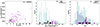 |
Fig. 1. Distribution of the general populations of (left) UDGs, (middle) LSBs, and (right) dIrrs in the space of their defining physical parameters: μg, 0 − Re, μB, 0, and MV, respectively. In each case, we denote the sample galaxies used for constructing dynamical models in black. The dotted lines indicate the ranges of respective parameters allowed for these galaxy classes. |
We followed the widely accepted definitions for the different galaxy types studied in this work, namely the UDGs, LSBs, and the dIrrs. It is true that the definitions of the different galaxy types are based on different physical parameters, namely surface brightness and stellar disc scale length for the UDGs, absolute magnitude for the dIrrs, and surface brightness for the LSBs. So, it may appear that one galaxy can be both an LSB and a dIrr at one time. Therefore, we compared and contrasted the distribution of the parent populations of the above galaxy types with respect to their B-band absolute magnitude. In Figure 2, we show the distribution of B-band absolute magnitude MB for all galaxies to study the possible overlap between different galaxy classes. The teal, yellow, and red histograms combine all the catalogues for the UDGs, LSBs, and the dIrrs, respectively. Although we do notice an overlap of the distributions, interestingly, the median values, as indicated by the empty triangles on the top, are fairly different in each case. In fact, the median B-band absolute magnitude of the LSB is starkly different from that of the dIrrs and the UDGs. Therefore, this indicates that a prototypical dIrr can never be a prototypical LSB and so on. Similarly, we should have compared the dIrrs and the LSBs with respect to the B-band central surface brightness distribution as well. However, information on the B-band central surface brightness is not available for the dIrr population. This is because the catalogues mostly provide information on the physical parameters on which the definition of the galaxy type is based. The full width at half maxima of the HI spectra (W50) serves as a proxy for the dynamical mass. For LSBs, it is 200 km s−1 (Matthews et al. 2001), and for dwarfs, it is 100 km s−1 (Karachentsev et al. 2001). However, we may note here that the median W50 value for the LSBs from de Blok et al. (1996) is about 120 km s−1. Therefore, it is reasonable to assume that LSBs and dIrrs constitute three different types of galaxies.
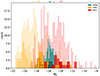 |
Fig. 2. Distribution of the UDGs, LSBs, and the dIrrs in the MB space with the UDGs, LSBs, and the dIrrs being represented by teal, yellow, and red colours, respectively. The empty and solid triangles on top of the plot represent the median MB, respectively, of the parent populations and the samples considered in our work. The galaxies were chosen from the literature as follows (ordered as the increasing shade of the histograms): (1) UDGs: Leisman et al. (2017); (2) LSBs: Impey et al. (1996), Kniazev et al. (2004), and de Blok et al. (1996); (3) dIrrs: Hunter & Elmegreen (2006) and van Zee & Haynes (2006). The histograms with black outlines represent the samples considered in our study. |
Finally, since the number of galaxies, considered in our study, was not large enough to carry out a statistical analysis similar to the PCA, we created mock galaxies corresponding to each galaxy in the samples for constructing dynamical models. We used the Monte Carlo (MC) method to generate the mock galaxy samples (for example, Raychaudhuri 2008). Considering the distribution of values of the different input parameters, 300 mock galaxies were generated from each original galaxy in a sample. Thus, we had an enlarged sample of 2100 galaxies for each of the UDG, LSB, and the dIrr populations. Further, we constructed dynamical models for each of these 2100 galaxies in each of our galaxy samples. The model kinematic parameters thus obtained, along with other structural parameters available in the literature, were used to carry out PCA.
5. Input parameters
We constructed the dynamical models of the original and mock galaxies using input as well as trial parameters from the mass models available in the literature. In the AGAMA framework, for generating the net potential of the stars, gas, and the dark matter halo, input parameters, namely (i) the dark matter core density (ρ0) and core radius (Rc) and (ii) the gas central surface density (ΣHI), scale radius (RD, HI) & scale height (hz, HI), as well as trial parameters for the DF of the stellar component, namely (iii) stellar central surface density (Σ0), exponential scale radius (RD), and scale height (hz, *) as well as stellar radial (σr) and vertical (σz) velocity dispersions are required.
For the UDGs, the dark matter halo and the gas disc parameters were taken from Kong et al. (2022); ΣHI and RD, HI were obtained by extracting data from the gas density plots presented in Kong et al. (2022) using HTML-based software WebPlotDigitizer1 and then fitting a sech-squared profile using the Python module SciPy. To set the dark matter halo potential for UDGs, the α, β, and γ values of Equation 5 were set according to the values listed in Table 2 of Kong et al. (2022). For the stellar component, we used the relation M* = 2πΣ0RD2 to calculate the stellar surface density of the galaxies, assuming their stellar disc component to be exponential in nature (Freeman 1970), M* and RD already presented by Mancera Piña et al. (2020). The central stellar surface density and stellar scale radius of the AGC242019, however, were obtained by fitting Σ* = Σ0exp(−R/RD) to the surface density profile presented by Shi et al. (2021). Similarly, for the LSBs, the dark matter halo parameters were taken from de Blok et al. (2001) and the gas disc parameters from de Blok et al. (1996). The central surface brightness values in B-band (μB, 0) and stellar scale radii were adopted from de Blok et al. (1996). The stellar surface brightness was converted to stellar surface density using the M/L ratio for the B-band as presented in Bell & de Jong (2001). Finally, for the dIrrs, we obtained the trial parameters of the stellar and gas components by extracting the data from the stellar and gas surface density profiles presented in Oh et al. (2015) and dark matter parameters from their Table 2. All these parameters for our sample galaxies are listed in Table A.1.
The stellar scale height hz is one of the trial parameters that is not observationally measured for our sample galaxies. However, for ordinary edge-on galaxies, hz has been found to lie between RD/5 and RD/7 (van der Kruit & Searle 1981). So, we chose a typical value of hz = RD/6 for our galaxy samples. Interestingly, we noted that there was hardly any variation in the profiles with the change in the assumed values of hz. This is because dispersion σ varies as hz0.5 in a self-gravitating system of stars in dynamical equilibrium, and so, the dependence of σ on the assumed value of hz may be understood to be weak, in general. Besides, the galaxy models were obtained by the iterative self-consistent method as described in Sect. 3, and thus the trial hz value could be considered as an initial guess for constructing the potential. Therefore, the error in the results due to the uncertainty in the hz values was also negligible.
Dynamical models for a sample of 5 dwarf galaxies by Banerjee et al. (2011) showed that the gas scale heights hz, HI at a mean radius (1.5RD) range between 0.2–0.4 kpc (0.1–0.4RD). Furthermore, Figure 7 of Mancera Piña et al. (2022a) indicates that the mean gas scale height of low-mass galaxies is about 0.2–0.6 kpc, which is similar to the range of values theoretically determined by Banerjee et al. (2011). So, we assumed a hz, HI of 0.25RD for our sample galaxies. We further checked and confirmed that our results hardly change if we vary the value of the assumed hz, HI between 0.1 and 0.4RD.
Finally, a trial value was used for σz in the DF based on the single-component model of a self-gravitating stellar disc,  (for example Mancera Piña et al. 2020) with h ∼ RD/6 (as discussed above). Similarly, σr was considered to be σz/0.3 (Gerssen & Shapiro Griffin 2012).
By trial-and-error method, we fine-tuned the value of σz such that the output hz from the self-consistent model of AGAMA lied between RD/5 > hz > RD/7 (in addition to complying with the observed total rotation curve and stellar surface density profiles).
We chose only a subset of the LSBs and the dIrrs studied in scaling relation to construct the dynamical models. The first selection criterion was based on the availability of the requisite stellar surface density and mass modelling data and the quality of fits of the exponential or sech-squared function to the surface density profiles to recover the input parameters for AGAMA. Further, we noted the decrease in the stellar central surface densities while constructing the dynamical models and rejected the galaxies with a decrease by more than 30% (as discussed in Sect. 3).
6. Methodology
6.1. Creation of mock galaxies
The mock galaxies generated from a parent galaxy represent a collection of galaxies with their physical parameters differing from those of the parent galaxy within the error bars. We chose one parent galaxy of our sample (Table A.1) and considered each of the ten input plus trial parameters {p1, p2, …, p10} of the galaxy (Sect. 5) to have a Gaussian distribution, with mean equal to the value corresponding to the parent galaxy and standard deviation equal to its error. From the multi-Gaussian distribution of {p1, p2, …, p10} thus obtained, we created a mock galaxy by randomly choosing ten parameters {p′1, p′2, …, p′10} by employing an MC simulation. Thus, 300 mock galaxies were generated from each of the parent galaxies. The dynamical models of these mock galaxies were constructed using AGAMA, the output of which was used in the PCA.
6.2. Principal component analysis
Principal component analysis (PCA) is used to understand the relative importance of the parameters in accounting for the variance in a given dataset (for reference Bro & Smilde 2014). In PCA, the covariance matrix in the chosen parameter space is solved, whose ith diagonal element describes the covariance of the ith parameter xi with itself, or the variance (cov(xi,xi)), and the ijth component gives the covariance between xi and xj (cov(xi,xj)), their respective expressions being:
In these expressions, each barred quantity denotes the mean value of the corresponding parameter and n is the number of data points taken into account. The eigenvectors of this matrix are the principal components, while their eigenvalues indicate the relative importance of the principal components. In principle, the data will cluster around the principal component with the largest eigenvalue in the principal component space, followed by the principal component with the second largest eigenvalue. Thus, if we project the data from the original space to the principal component space, we see variation in the data is mainly explained by the first two principal components with the largest eigenvalues, thus leading to a dimensionality reduction. The principal components can be considered as linear combinations of the original variables, and the coefficients of their variables are called loadings. Variable corresponding to the largest loading primarily describes variance in the data.
To obtain the PCA loading values, we followed these steps: we (1) performed PCA analysis with the largest possible set of the structural and kinematical parameters for each galaxy-class; (2) took the vector sum of the first two principal components with the largest eigenvalues; (3) identified the parameter that has the largest loading value and normalised other loadings by the largest one; (4) eliminated the parameters with negligible loading values and repeated the procedure until the results converged. In all the cases, we saw that the first two principal components explain nearly 80–90% of the variance in the data. Finally, we ended up with the most relevant set of structural and kinematic parameters to study the dynamics of our galaxy samples. We employed the sklearn module in Python to perform the principal component analysis.
7. Results and discussion
We present the results in three subsections. In Sect. 7.1, we looked for correlations between pairs of basic structural properties for our LSB and dIrr populations and checked if our sample UDGs comply with either of them. In Sect. 7.2, we constructed dynamical models of our sample UDGs, LSBs, and dIrrs and compared their model-predicted stellar kinematics. Finally, in Sect. 7.3, we carried out a PCA analysis for a set of structural and kinematic properties of each of our galaxy populations to identify the crucial parameters explaining the variance in their respective datasets.
7.1. Possible galaxy scaling relations
In Figure 3, we compared the results of statistical analysis of the physical properties of the UDGs, LSBs, and the dIrrs. For each pair of parameters, we determined the respective regression line fits with the 68% (∼1-standard deviation) confidence intervals for our sample LSBs and dIrrs and superposed the data for our UDGs on these. The error bars for the UDG data points were obtained from Mancera Piña et al. (2020) and Kong et al. (2022) or evaluated by propagation of error. We did not consider the error bars for most of the regression fits, as these are not available for most of these parameters. We noted the R-squared (R2) value to measure the quality of the regression fit and rejected the scaling relation for which the R2 < 0.25. We used the Python module statsmodels to obtain the scaling relations, fitting parameters, and R2 s. We obtained the standard error in R2 from a set of R2 s, each obtained by fitting regression to a simulated dataset generated from the original one by bootstrapping with replacement. Further, to check whether the UDGs comply with the regression fit of the LSB or the dIrr population, we did the following statistical test. For the pair of parameters (X,Y) involved in each of the scaling relations, we randomly chose 100 values of X in the same range as the X values of the UDG population. For each value of X so chosen, we generated the corresponding Y value by randomly choosing it from a Gaussian distribution centred at the Y value from the regression fit and standard deviation equal to half of the 68% confidence interval from the mean. Thus, we generated a simulated dataset of 100 elements for each of the LSB and the dIrr populations. Further, we conducted a two-sample Anderson-Darling (AD) test between the simulated LSB (dIrr) sample and the UDG sample and noted the p-value and the AD coefficient. We repeated this process 10 000 times and noted the mean p-value and AD-coefficient ( ,
,  ,
,  , and
, and  , respectively). The standard error in p is mentioned unless negligible. The
  -value indicates the probability of the null hypothesis that the two samples are drawn from the same population. A
  -value < 0.02 indicates that the two populations are significantly different from each other. On the other hand, the alternative hypothesis that the two samples are drawn from the same normal distribution cannot be ruled out for
  > 0.02. Additionally, we compared
  with the critical AD-coefficient (ADcrit) for the sample sizes of the two populations considered in the AD test (Pettitt 1976). In all the cases, our ADcrit has a value of 2.718 at a significance level of 2.5 percent. For
  , the null hypothesis is rejected. We used the SciPy module in Python to perform these tests.
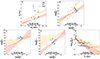 |
Fig. 3. Scaling relations between several mass and structural properties of our galaxy samples. In the top row, (a) HI diameter versus exponential stellar scale radius (DHI vs. RD), (b) stellar mass versus HI mass (log M* vs. log MHI); in the bottom row, (c) total baryonic mass versus total dynamical mass enclosed in within 4 RD (log Mb vs. log Mdyn), (d) stellar mass versus total dynamical mass (log M* vs. log Mdyn), (e) dark matter core density versus core density (ρ0 vs. Rc). In all plots, the regression fits for LSBs and dIrrs with their 68% (1-standard deviation) confidence intervals are shown in yellow and red, respectively, and the data for UDGs are superposed on their regression fits with teal stars. The R2 values for the regression fit for LSBs and dIrrs (RLSB2 and RdIrr2, respectively) are mentioned at the bottom of each plot. Also, |


We show the exponential scale radii (RD) versus HI diameters (DHI) distribution for our sample UDGs, LSBs, and dIrrs in panel (a). It is well known that, similar to dIrrs and LSBs, field UDGs have remarkably high HI masses for their stellar content (Trujillo et al. 2017; Mancera Piña et al. 2020). For normal spiral galaxies, the ratio of the HI-to-optical diameter is nearly 2 (Broeils & Rhee 1997), yet there are several galaxies that have unusually extended HI discs (Begum et al. 2005; Gentile et al. 2007; Wang et al. 2016). The extended HI disc can be attributed to gas accretion or merger, though the origin of such large gas discs is still debatable (Noordermeer et al. 2005). The HI mass (MHI) and diameter (DHI) of a galaxy have been found to be correlated as follows: log DHI = 0.506 log MHI − 3.293 (Broeils & Rhee 1997; Wang et al. 2016). UDGs in our galaxy sample, except AGC242019, follow the DHI–MHI relation of Wang et al. (2016) (Gault et al. 2021). We used this relation to obtain the DHI of the galaxies and obtained the RD–DHI scaling relation. The R2 for the regression fits for LSBs and dIrrs are, respectively, 0.462 and 0.415. In this context, we mention that for all the regression fits discussed in this section, the standard error of R2 is negligible (∼10−5). Further, we did an AD test to check if the UDGs comply with the scaling relation of the dIrr or the LSB. Both  and
and  have a value equal to 0.001 for this scaling relation, meaning that the UDGs do not follow any of their normal distribution as far as the RD–DHI scaling relation is concerned. A similar conclusion can be drawn by observing that both
  (6.88 ± 0.64) and
  (7.81 ± 0.74) are greater than ADcrit.
In panel (b), we present the correlation between the stellar mass (M*) and the HI mass (MHI) of the LSBs and the dIrrs for which the R2 values are, respectively, 0.535 and 0.418. We note that  and
and  are again 0.001 and 21.5 ± 0.06 for this scaling relation, thus rejecting the null hypothesis. However,
  is 0.19 ± 0.06 and
  is 0.54 ± 0.54, suggesting that the UDGs and dIrrs may follow similar normal distributions. Although the range of HI masses of the UDGs is the same as the LSBs, they, however, obey the same M*–MHI scaling relation as the dIrrs. Since star formation rate increases with increasing stellar mass, UDGs and dIrrs will have relatively smaller star formation rates than the LSBs (Figure 8 of Zhou et al. 2018). Hence, the extraordinarily low surface brightness of UDGs may be attributed to inefficient star formation in these galaxies (as suggested by McGaugh & de Blok (1997a) and Impey & Bothun (1997) for LSBs).
Since dwarf galaxies are dark matter dominated at all radii, dark matter plays an important role in their dynamics and can be crucial to explain their low luminosity (Read et al. 2016, 2017; Mancera Piña et al. 2022b). Garg & Banerjee (2017) showed that dark matter suppresses the local axisymmetric instabilities, which, in turn, may lower the star formation rate in a galaxy, leading to a lower surface brightness. Hence, in the bottom row of Figure 3, we discuss the correlations between dynamical parameters that may explain the role of dark matter in regulating their evolution.
In panel (c), we present the respective regression fits between baryonic (Mb) and dynamical (Mdyn) mass with the 1σ-confidence intervals for the LSBs and the dIrrs. The dynamical mass is taken to be the mass enclosed within the radius of 4 times the stellar scale radius RD ( = 4V∞2RD/G), the baryonic mass being M* + 1.33 MHI (1.33 being the helium correction factor). This is analogous to the baryonic Tully-Fisher relation (BTFR), where the dynamical mass is considered as a proxy of their circular velocity (McGaugh et al. 2000; McGaugh 2005). The R2 for the regression fits for LSBs and dIrrs are, respectively, 0.262 and 0.355. Similar to panel (a), ( ,
,  ) and
) and  have values (0.001, 0.001) and (15.71 ± 1.74, 17.15 ± 1.67), respectively, thus suggesting that the UDGs constitute a distinct class of galaxies, relatively baryon-dominated, lying above the BTFR as discussed in Mancera Piña et al. (2019b).
In panel (d), we show the correlation between stellar mass (M*) and dynamical mass (Mdyn) for our galaxy samples. The R2 values for the regression fits of the LSBs and the dIrrs are 0.317 and 0.487, respectively. We note that the value of  and
and  = 11.18 ± 1.73, from which we may infer that the UDGs and the LSBs are members of two different populations. However,
  is 0.08 ± 0.04 and
  is −1.63 ± 0.59; thus, we cannot decline the possibility that the UDGs and the dIrrs may belong to a similar galaxy population. This is in line with the fact that the dIrrs share similar stellar and dynamical mass ranges, with the UDGs having slightly higher values than that of the dIrrs. In a way, the M* and Mdyn scaling relation indicates the star formation rate as a function of the dark matter mass of a galaxy. Hence, the difference in their correlation may imply the difference in the way the dark matter regulates the star formation rate.
Finally, in panel (e), we present the correlation between dark matter core density (ρ0) and core radius (Rc), which is routinely used to study the dark matter dominance in galaxies (de Blok et al. 2001; Banerjee & Bapat 2017). The error bars for the halo core radius are obtained from Kong et al. (2022), de Blok et al. (2001), and Oh et al. (2015), respectively, for the UDGs, LSBs, and the dIrrs. We obtained the weighted regression fits for the LSBs and dIrrs using the Python module statsmodels and the corresponding R2 equal to 0.573 and 0.408, respectively. Based on the values of  and
and  ), we conclude that the UDGs and the LSBs are very different from each other with respect to their dark matter distributions. However,
  and
and  ADcrit) indicate that the UDGs and the dIrrs may follow the same normal distribution and hence evolve under similar dark matter halo potentials. Further, we observe that, for a given ρ0 value, the LSBs have more cuspy halos compared to the UDGs and the dIrrs.
Considering the comparison of all the scaling relations above, we may say that UDGs constitute a different population as far as the LSBs are concerned. However, one cannot completely rule out the possibility of UDGs and dIrrs being one and the same population.
7.2. Stellar kinematics from dynamical modelling using AGAMA
Stellar kinematics constitute a primary diagnostic tracer of the dynamical and secular evolution of a galaxy (Pinna et al. 2018). We generated galaxy models for our UDG, LSB, and dIrr samples using the input parameters listed in Table A.1 employing AGAMA. We constrained the galaxy models by the observed rotation curve and surface density profiles. To check the consistency between the galaxy models and the observed profiles, we compared and contrasted the model-predicted rotation curves and stellar surface density profiles with the observed ones. In Figure 4, we present the observed profile by points and the model-obtained profiles with solid lines. For the stellar surface density of the UDGs and the LSBs, we reconstructed the exponential profile from their central surface density and stellar scale radius given in the literature. These are shown with the dotted lines. We note that the central values of the stellar surface density are slightly smaller compared to their observed profile (as discussed in Sect. 3).
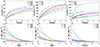 |
Fig. 4. Comparison between model (solid lines) and observed (scatter data points/dotted lines) (i) rotation curves (top panel) and (ii) stellar surface density profiles (bottom panel), for the UDGs (left), LSBs (middle), and the dIrrs (right). |
In the top panel of Figure 5, we plot stellar σr/σz at a few galactocentric radii R normalised by their exponential stellar disc scale length RD, for our sample of UDGs, LSBs, and dIrrs. σr/σz may indicate the relative dominance of stellar disc heating in the radial versus the vertical direction. While σz is mostly regulated by vertical bending instabilities (for example, Łokas 2019), σr is governed by radial heating due to disc non-axisymmetric features such as bars and spiral arms (Pinna et al. 2018 and the citations therein). According to Shapiro et al. (2003), late-type galaxies have σz/σr< 0.5 (or, σr/σz > 2), while early-type galaxies have σr/σz < 2. We observe that at almost all radii, the σr/σz values of the UDGs range between 1.5 and 3, and the corresponding values for the dIrrs seem to mostly overlap with them. While on the other hand, the average σz/σr for the LSB population is relatively higher, lying between 2.5 and 3 consistently at all radii. In addition, we conducted a statistical test to quantitatively assess the similarities between the kinematic parameters of two galaxy samples. For each galaxy sample, we resampled the data of σz/σr at a galactocentric radius by bootstrapping with replacement to increase the sample size to 100. Next, we performed the non-parametric Mann-Whitney U-test between the UDGs and the LSBs (dIrrs) considering the σz/σr-values at one radius and then noted the corresponding p-value, pLSB (pdIrr). We repeated the process 1000 times at each of the 20 radial points between 0 and 4RD and then obtained the median p-value,  (
( ) at each radius. We note that
  and
and  values are of the order of 10−26 and 10−26, respectively, that as far as the shape of the stellar velocity ellipsoids are concerned, UDGs, LSBs, and dIrrs constitute different populations.
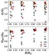 |
Fig. 5. Ratios of the stellar radial-to-vertical velocity dispersion (σr/σz), obtained from AGAMA at 1RD, 1.5RD, 2RD, and 2.5RD plotted for UDGs, LSBs, and dIrrs are shown in the top panel. In the bottom panel, circular-to-total stellar velocity dispersion ratios (VROT/σ0) are presented at the same radii as the top panel. |
In the bottom panel of Figure 5, we present the ratio of the rotational velocity-to-the-total stellar velocity dispersion (VROT/σ0). VROT/σ0 is a measure of the angular momentum-to-random motion support against gravitational collapse in a galaxy (Toloba et al. 2009; Fraser-McKelvie & Cortese 2022). Falcón-Barroso et al. (2019) found that elliptical galaxies have relatively lower values of VROT/σ0, which increases as we move from left to right in the Hubble sequence. Low and high values of VROT/σ0 indicate slow and fast rotators, respectively. We note that at the inner radii, VROT/σ0 values for the LSBs lie between 0.7 and 1, while at the intermediate and the outer radii, the value is close to 1, indicating that LSBs are fast rotators. This is in line with their late-type kinematics found above. For the dIrrs and the UDGs, the average value of VROT/σ0 lies around 0.5 at the inner radii. At the intermediate and outer radii, the average VROT/σ0 for the dIrrs are 0.8 and 0.9, respectively, though with a large variance. For the UDGs, the corresponding values are about 0.6, again with a fairly large scatter. Further, we conducted the Mann-Whitney U-test and noted the  and
and  values. We observe that
  and
and  have values very close to 0, thus rejecting the hypothesis that the UDGs and LSBs (dIrrs) constitute the same population.
Therefore, we conclude that UDGs, LSBs, and dIrrs are very different as far as their model-predicted kinematics is concerned. Here, we emphasise the fact that the values of σr/σz and VROT/σ0 presented in this section are obtained from their dynamical models.
7.3. The key dynamical parameters of our galaxy samples: Principal component analysis
Finally, in Figure 6, we present the results obtained from the PCA of a set of dynamical parameters possibly driving their disc dynamics for each of our galaxy samples. We chose the following set of dynamical parameters from our mock galaxy models (as described in Sect. 6).
-
Ratio of stellar central surface density to scale radius (Σ0/RD): By definition, UDGs have very low central surface brightness with relatively large effective radii compared to other low surface brightness galaxies (van Dokkum et al. 2015a). Thus, we may consider the ratio of stellar surface density to stellar scale radius as a possible defining parameter of UDGs.
-
Stellar mass (M*): The stars constitute one of three basic building blocks of a galaxy, the others being the gas and dark matter halo. The stellar mass correlates with the dark matter mass as well as with the star-formation histories, thus revealing key information about the formation and evolution of the galaxy (Conroy & Wechsler 2009).
-
Atomic hydrogen mass (MHI): MHI correlates with several fundamental galaxy properties, thus serving as a fingerprint of the stage of evolution of a galaxy (McGaugh & de Blok 1997b). It was observed that the correlation between galaxy gas content and the central surface brightness of disc galaxies is the strongest, making MHI a crucial dynamical component, especially for low-surface brightness galaxies.
-
Asymptotic velocity (V∞): V∞ has a tight correlation with the total baryonic mass of a galaxy through the baryonic Tully-Fisher relation. Moreover, V∞ can be considered as a proxy of the total dynamical mass of a galaxy and hence can be considered as a dynamical parameter, as understood and seen in previous studies (Aditya et al. 2023). We considered the value of mean velocity at a radius equal to 4RD as the asymptotic velocity.
-
Specific angular momentum (j*): Specific angular momentum is one of the fundamental dynamical parameters of a galaxy that traces the accretion history of the gas disc, thus revealing important information about its formation and evolution. There is a strong correlation between the stellar specific angular momentum and the stellar mass of the galaxies followed by various morphological types observed over different redshifts (Fall 1983; Romanowsky & Fall 2012). In this connection, we note that correlations between mass, stellar specific angular momentum, and gas fraction/central surface density were observed by Mancera Piña et al. (2021b) and Elson (2024). We calculated the specific angular momentum employing the following expression:
We considered an exponential stellar surface density profile Σ*(R) and velocity profile to be v(R) = V0[1 − exp(−R/a)] (V0 and a being the fitting parameters of the rotation curve). In our study, we calculated j* by considering the model-derived stellar surface density and rotation velocity profiles. We performed the integration between 0 to ∞ using the Python module SciPy.
-
Total stellar velocity dispersion (σ): Rotation-supported self-gravitating discs are unstable against gravitational instabilities and random motion of stars quantified by velocity dispersion of the disc is crucial for their stability, as indicated by the Toomre-Q parameter (Toomre & Rott 1964). Furthermore, the total stellar velocity dispersion shows a correlation with the dark matter halo mass, thus implying dark matter dominance in galaxy evolution (Zahid et al. 2018). AGAMA over-predicts the central surface density due to the caveat discussed in Sect. 3. Thus, we considered the total stellar velocity dispersion value at 1.5 RD, where the model-obtained stellar surface density distribution matches the observed profile fairly well (Figure 4).
-
Stellar radial-to-vertical velocity dispersion
 : Stellar velocity ellipsoid (SVE) constitutes a fingerprint of the disc heating mechanisms of a galaxy. σr/σz quantifies the flattening of the SVE and can be considered as an indicator of the secular evolution of a galaxy (van der Kruit & de Grijs 1999). For PCA, we considered the value of σr/σz at 1.5 RD, as it should be representative of the mean kinematics of the disc.
 -
Compactness parameter
 : The ratio of dark matter core radius-to-exponential stellar disc scale length (Rc/RD) can be considered an indicator of the compactness of the dark matter halo, with Rc/RD≥ 2 and Rc/RD≤ 2 indicating non-compact and compact dark matter halos, respectively (Gentile et al. 2004; Banerjee & Jog 2008, 2013; Banerjee et al. 2010). Aditya et al. (2023) extended this definition further by introducing the ratio of asymptotic velocity (V∞) and Rc/RD as the compactness of mass distribution. The dynamical masses of low-luminosity galaxies are primarily dominated by dark matter at all radii. Hence, V∞/(Rc/RD) indicates the compactness of mass distribution within the central region of the galaxies. The larger the value of V∞/(Rc/RD), the more compact the mass distribution. The compactness of mass distribution is argued to be an important parameter to understand the stability of superthin stellar discs (Aditya et al. 2023 and references therein).
In Figure 6, from left to right, we present the sum of the first two loadings of the PCA corresponding to our UDGs, LSBs, and dIrrs, which account for ∼87%, 79%, and 83% variance in the data, respectively. We observe that, for the UDGs, M*, MHI, and then Σ0/RD can explain the maximum variance in the data. For dIrrs, the important parameters are MHI and M*, followed by σr/σz. As observed by Mancera Piña et al. (2020), the mass fraction of dark matter in UDGs is relatively low, and therefore, it is not surprising that MHI and M* have emerged as the fundamental dynamical parameters for the UDGs from the PCA analysis. We conclude that for both the UDGs and the dIrrs, MHI and M* play key roles in regulating the disc dynamics, as is evident from the PCA analysis of their dynamical parameters. However, j* also appears to be a crucial parameter for the dIrrs but not for UDGs. This is in contradiction to the predictions of Amorisco & Loeb (2016), Mancera Piña et al. (2020), and Benavides et al. (2023), who argued that UDGs are possibly hosted in high-spin dark matter halos that may regulate their formation scenario. Curiously, this is in compliance with the findings by Bellazzini et al. (2017), where they reported the discovery of two field dIrrs, SdI-1 and SdI-2, which closely follow the properties of UDGs. Though their spectroscopic images reveal remarkable irregular features, their sizes are comparable to UDGs, as demonstrated by their V-band magnitude-effective radii distribution, and hence in further studies they are considered to be isolated UDGs (for example, Papastergis et al. 2017). For LSBs, on the other hand, σr/σz, MHI, and V∞ mostly explain the variance in the data.
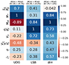 |
Fig. 6. Loadings corresponding to the first two principal components are presented for each of our UDG, LSB, and dIrr galaxy samples, which account for at least 80% of the variation in the data. Parameters considered in this analysis from top to bottom are as follows: the ratio of stellar central surface density-to-exponential stellar scale radius (Σ0/RD), stellar mass (M*), HI mass (MHI), the ratio of stellar radial-to-vertical velocity dispersion (σr/σz), asymptotic velocity (V∞), the compactness parameter (V∞/(Rc/RD)), stellar velocity dispersion (σ), and specific angular momentum (j*). |
8. Conclusions
In this work, we studied the dynamical lineage of isolated, HI-rich UDGs and looked for a possible common origin with other low-luminosity galaxies, namely the LSBs and the dIrrs. We considered a sample of galaxies for each of the above galaxy populations and first constructed possible scaling relations between pairs of structural and kinematical parameters, as obtained from the literature. We then obtained separate regression fits for the LSB and the dIrr data with the corresponding 68% confidence intervals and superposed the data points for the UDGs on them. We further conducted two-sample Anderson-Darling tests to check the similarities among UDGs, LSBs, and dIrr samples. We observe that the UDGs and the LSBs constitute statistically different populations. However, based on the stellar mass versus HI mass (log M*–log MHI), stellar mass versus total dynamical mass (log M*–log Mdyn), and dark matter core density and core radius (ρ0–Rc) fits, we cannot rule out the possibility of the UDGs and the dIrr populations following the same normal distributions. Further, we constructed their dynamical models employing the publicly available stellar dynamical code AGAMA as constrained by their mass models already available in the literature. A Mann-Whitney U-test on the distribution of the kinematical parameters, namely ratios of radial-to-vertical stellar velocity dispersion and the rotational velocity-to-total stellar velocity dispersion, indicates that the UDGs, the LSBs, and the dIrrs constitute starkly different populations. Finally, we carried out a principal component analysis of a fixed set of structural and kinematical parameters for each galaxy population that plausibly regulates their disc dynamics. We find that the variance in the data of the UDGs and the dIrrs is mostly explained by a common set of parameters, namely, the total HI mass and the stellar mass. For the LSBs, that is accounted for by the radial-to-vertical stellar velocity dispersion ratio, followed by the HI mass. Therefore, considering the above, isolated, HI-rich UDGs seem to share a common dynamical lineage with the dIrrs but not so much with the LSBs.
Acknowledgments
We acknowledge that the project is funded by the Prime Minister’s Research Fellowship with ID: 0902007. We thank the anonymous referee for the detailed, constructive suggestions, which have improved the paper. We also thank Prof. Nissim Kanekar for useful discussions and suggestions.
References
- Aditya, K., Banerjee, A., Kamphuis, P., et al. 2023, MNRAS, 526, 29 [NASA ADS] [CrossRef] [Google Scholar]
- Afanasiev, A. V., Chilingarian, I. V., Grishin, K. A., et al. 2023, MNRAS, 520, 6312 [CrossRef] [Google Scholar]
- Amorisco, N. C., & Loeb, A. 2016, MNRAS, 459, L51 [NASA ADS] [CrossRef] [Google Scholar]
- Banerjee, A., & Bapat, D. 2017, MNRAS, 466, 3753 [NASA ADS] [CrossRef] [Google Scholar]
- Banerjee, A., & Jog, C. J. 2008, ApJ, 685, 254 [Google Scholar]
- Banerjee, A., & Jog, C. J. 2013, MNRAS, 431, 582 [NASA ADS] [CrossRef] [Google Scholar]
- Banerjee, A., Matthews, L. D., & Jog, C. J. 2010, New Astron., 15, 89 [NASA ADS] [CrossRef] [Google Scholar]
- Banerjee, A., Jog, C. J., Brinks, E., & Bagetakos, I. 2011, MNRAS, 415, 687 [NASA ADS] [CrossRef] [Google Scholar]
- Barbosa, C. E., Zaritsky, D., Donnerstein, R., et al. 2020, ApJS, 247, 46 [Google Scholar]
- Begum, A., Chengalur, J. N., & Karachentsev, I. D. 2005, A&A, 433, L1 [NASA ADS] [CrossRef] [EDP Sciences] [Google Scholar]
- Bell, E. F., & de Jong, R. S. 2001, ApJ, 550, 212 [Google Scholar]
- Bellazzini, M., Belokurov, V., Magrini, L., et al. 2017, MNRAS, 467, 3751 [NASA ADS] [Google Scholar]
- Benavides, J. A., Sales, L. V., Abadi, M. G., et al. 2023, MNRAS, 522, 1033 [NASA ADS] [CrossRef] [Google Scholar]
- Boissier, S., Monnier Ragaigne, D., Prantzos, N., et al. 2003, MNRAS, 343, 653 [NASA ADS] [CrossRef] [Google Scholar]
- Bothun, G., Impey, C., & McGaugh, S. 1997, PASP, 109, 745 [NASA ADS] [CrossRef] [Google Scholar]
- Bro, R., & Smilde, A. K. 2014, Anal. Methods, 6, 2812 [CrossRef] [Google Scholar]
- Broeils, A. H., & Rhee, M. H. 1997, A&A, 324, 877 [NASA ADS] [Google Scholar]
- Brook, C. B., Di Cintio, A., Macciò, A. V., & Blank, M. 2021, ApJ, 919, L1 [NASA ADS] [CrossRef] [Google Scholar]
- Chilingarian, I. V., Afanasiev, A. V., Grishin, K. A., Fabricant, D., & Moran, S. 2019, ApJ, 884, 79 [NASA ADS] [CrossRef] [Google Scholar]
- Conroy, C., & Wechsler, R. H. 2009, ApJ, 696, 620 [NASA ADS] [CrossRef] [Google Scholar]
- Conselice, C. J. 2018, Res. Notes Am. Astron. Soc., 2, 43 [Google Scholar]
- da Costa, L. N., & Renzini, A. 1997, Galaxy Scaling Relations: Origins, Evolution and Applications. Proceedings (Berlin: Springer) [CrossRef] [Google Scholar]
- Dalcanton, J. J., Spergel, D. N., & Summers, F. J. 1997, ApJ, 482, 659 [NASA ADS] [CrossRef] [Google Scholar]
- Danieli, S., van Dokkum, P., Conroy, C., Abraham, R., & Romanowsky, A. J. 2019, ApJ, 874, L12 [NASA ADS] [CrossRef] [Google Scholar]
- de Blok, W. J. G., McGaugh, S. S., & van der Hulst, J. M. 1996, MNRAS, 283, 18 [NASA ADS] [CrossRef] [Google Scholar]
- de Blok, W. J. G., McGaugh, S. S., & Rubin, V. C. 2001, AJ, 122, 2396 [NASA ADS] [CrossRef] [Google Scholar]
- Du, L., Du, W., Cheng, C., et al. 2024, ApJ, 964, 85 [NASA ADS] [CrossRef] [Google Scholar]
- Efstathiou, G., & Silk, J. 1983, Fund. Cosmic Phys., 9, 1 [NASA ADS] [Google Scholar]
- Elson, E. 2024, MNRAS, 527, 931 [Google Scholar]
- Falcón-Barroso, J., van de Ven, G., Lyubenova, M., et al. 2019, A&A, 632, A59 [Google Scholar]
- Fall, S. M. 1983, Internal Kinematics and Dynamics of Galaxies, 391 [CrossRef] [Google Scholar]
- For, B. Q., Spekkens, K., Staveley-Smith, L., et al. 2023, ArXiv e-prints [arXiv:2309.11799] [Google Scholar]
- Forbes, D. A., Gannon, J., Couch, W. J., et al. 2019, A&A, 626, A66 [NASA ADS] [CrossRef] [EDP Sciences] [Google Scholar]
- Fraser-McKelvie, A., & Cortese, L. 2022, ApJ, 937, 117 [NASA ADS] [CrossRef] [Google Scholar]
- Freeman, K. C. 1970, ApJ, 160, 811 [Google Scholar]
- Garg, P., & Banerjee, A. 2017, MNRAS, 472, 166 [NASA ADS] [CrossRef] [Google Scholar]
- Gault, L., Leisman, L., Adams, E. A. K., et al. 2021, ApJ, 909, 19 [NASA ADS] [CrossRef] [Google Scholar]
- Gentile, G., Salucci, P., Klein, U., Vergani, D., & Kalberla, P. 2004, MNRAS, 351, 903 [Google Scholar]
- Gentile, G., Salucci, P., Klein, U., & Granato, G. L. 2007, MNRAS, 375, 199 [CrossRef] [Google Scholar]
- Gerssen, J., & Shapiro Griffin, K. 2012, MNRAS, 423, 2726 [NASA ADS] [CrossRef] [Google Scholar]
- Hu, H.-J., Guo, Q., Zheng, Z., et al. 2023, ApJ, 947, L9 [NASA ADS] [CrossRef] [Google Scholar]
- Hunter, D. A., & Elmegreen, B. G. 2006, VizieR Online Data Catalog: J/ApJS/162/49 [Google Scholar]
- Hunter, D. A., Hunsberger, S. D., & Roye, E. W. 2000, ApJ, 542, 137 [NASA ADS] [CrossRef] [Google Scholar]
- Ikeda, R., Morishita, T., Tsukui, T., et al. 2023, MNRAS, 523, 6310 [NASA ADS] [CrossRef] [Google Scholar]
- Impey, C., & Bothun, G. 1997, ARA&A, 35, 267 [NASA ADS] [CrossRef] [Google Scholar]
- Impey, C., Bothun, G., & Malin, D. 1988, ApJ, 330, 634 [Google Scholar]
- Impey, C. D., Sprayberry, D., Irwin, M. J., & Bothun, G. D. 1996, ApJS, 105, 209 [Google Scholar]
- Jadhav Y, V., & Banerjee, A. 2019, MNRAS, 488, 547 [NASA ADS] [CrossRef] [Google Scholar]
- Janssens, S., Abraham, R., Brodie, J., et al. 2017, ApJ, 839, L17 [NASA ADS] [CrossRef] [Google Scholar]
- Janssens, S. R., Abraham, R., Brodie, J., Forbes, D. A., & Romanowsky, A. J. 2019, ApJ, 887, 92 [Google Scholar]
- Karachentsev, I. D., Karachentseva, V. E., & Huchtmeier, W. K. 2001, A&A, 366, 428 [NASA ADS] [CrossRef] [EDP Sciences] [Google Scholar]
- Karunakaran, A., Spekkens, K., Zaritsky, D., et al. 2020, ApJ, 902, 39 [CrossRef] [Google Scholar]
- Kim, J.-H., & Lee, J. 2013, MNRAS, 432, 1701 [Google Scholar]
- Kniazev, A. Y., Grebel, E. K., Pustilnik, S. A., et al. 2004, AJ, 127, 704 [NASA ADS] [CrossRef] [Google Scholar]
- Kong, D., Kaplinghat, M., Yu, H.-B., Fraternali, F., & Mancera Piña, P. E. 2022, ApJ, 936, 166 [NASA ADS] [CrossRef] [Google Scholar]
- Leaman, R., Venn, K. A., Brooks, A. M., et al. 2012, ApJ, 750, 33 [NASA ADS] [CrossRef] [Google Scholar]
- Lee, H., McCall, M. L., & Richer, M. G. 2003, AJ, 125, 2975 [NASA ADS] [CrossRef] [Google Scholar]
- Leisman, L., Haynes, M. P., Janowiecki, S., et al. 2017, ApJ, 842, 133 [NASA ADS] [CrossRef] [Google Scholar]
- Łokas, E. L. 2019, A&A, 629, A52 [NASA ADS] [CrossRef] [EDP Sciences] [Google Scholar]
- Mancera Piña, P. E., Aguerri, J. A. L., Peletier, R. F., et al. 2019a, MNRAS, 485, 1036 [CrossRef] [Google Scholar]
- Mancera Piña, P. E., Fraternali, F., Adams, E. A. K., et al. 2019b, ApJ, 883, L33 [CrossRef] [Google Scholar]
- Mancera Piña, P. E., Fraternali, F., Oman, K. A., et al. 2020, MNRAS, 495, 3636 [Google Scholar]
- Mancera Piña, P. E., Posti, L., Fraternali, F., Adams, E. A. K., & Oosterloo, T. 2021a, A&A, 647, A76 [NASA ADS] [CrossRef] [EDP Sciences] [Google Scholar]
- Mancera Piña, P. E., Posti, L., Pezzulli, G., et al. 2021b, A&A, 651, L15 [NASA ADS] [CrossRef] [EDP Sciences] [Google Scholar]
- Mancera Piña, P. E., Fraternali, F., Oosterloo, T., et al. 2022a, MNRAS, 514, 3329 [CrossRef] [Google Scholar]
- Mancera Piña, P. E., Fraternali, F., Oosterloo, T., et al. 2022b, MNRAS, 512, 3230 [CrossRef] [Google Scholar]
- Mancera Piña, P. E., Golini, G., Trujillo, I., & Montes, M. 2024, A&A, 689, A344 [NASA ADS] [CrossRef] [EDP Sciences] [Google Scholar]
- Martin, G., Kaviraj, S., Laigle, C., et al. 2019, MNRAS, 485, 796 [NASA ADS] [CrossRef] [Google Scholar]
- Martínez-Delgado, D., Läsker, R., Sharina, M., et al. 2016, AJ, 151, 96 [CrossRef] [Google Scholar]
- Matthews, L. D., van Driel, W., & Monnier-Ragaigne, D. 2001, A&A, 365, 1 [NASA ADS] [CrossRef] [EDP Sciences] [Google Scholar]
- McGaugh, S. S. 2005, ApJ, 632, 859 [Google Scholar]
- McGaugh, S., & de Blok, E. 1997a, AIP Conf. Ser., 393, 510 [NASA ADS] [CrossRef] [Google Scholar]
- McGaugh, S. S., & de Blok, W. J. G. 1997b, ApJ, 481, 689 [NASA ADS] [CrossRef] [Google Scholar]
- McGaugh, S. S., Schombert, J. M., Bothun, G. D., & de Blok, W. J. G. 2000, ApJ, 533, L99 [Google Scholar]
- Mo, H. J., Mao, S., & White, S. D. M. 1998, MNRAS, 295, 319 [Google Scholar]
- Mo, H., van den Bosch, F. C., & White, S. 2010, Galaxy Formation and Evolution (Cambridge, UK: Cambridge University Press) [Google Scholar]
- Müller, O., Jerjen, H., & Binggeli, B. 2018, A&A, 615, A105 [Google Scholar]
- Narayanan, G., & Banerjee, A. 2022, MNRAS, 514, 5126 [NASA ADS] [CrossRef] [Google Scholar]
- Noordermeer, E., van der Hulst, J. M., Sancisi, R., Swaters, R. A., & van Albada, T. S. 2005, A&A, 442, 137 [NASA ADS] [CrossRef] [EDP Sciences] [Google Scholar]
- Oh, S.-H., Hunter, D. A., Brinks, E., et al. 2015, AJ, 149, 180 [CrossRef] [Google Scholar]
- O’Neil, K., Bothun, G., van Driel, W., & Monnier Ragaigne, D. 2004, A&A, 428, 823 [CrossRef] [EDP Sciences] [Google Scholar]
- Papastergis, E., Adams, E. A. K., & Romanowsky, A. J. 2017, A&A, 601, L10 [NASA ADS] [CrossRef] [EDP Sciences] [Google Scholar]
- Pérez-Montaño, L. E., & Cervantes Sodi, B. 2019, MNRAS, 490, 3772 [CrossRef] [Google Scholar]
- Pettitt, A. N. 1976, Biometrika, 63, 161 [Google Scholar]
- Pinna, F., Falcón-Barroso, J., Martig, M., et al. 2018, MNRAS, 475, 2697 [NASA ADS] [CrossRef] [Google Scholar]
- Pokhrel, N. R., Simpson, C. E., & Bagetakos, I. 2020, AJ, 160, 66 [NASA ADS] [CrossRef] [Google Scholar]
- Poulain, M., Marleau, F. R., Habas, R., et al. 2022, A&A, 659, A14 [NASA ADS] [CrossRef] [EDP Sciences] [Google Scholar]
- Prole, D. J., van der Burg, R. F. J., Hilker, M., & Davies, J. I. 2019, MNRAS, 488, 2143 [NASA ADS] [Google Scholar]
- Prole, D. J., van der Burg, R. F. J., Hilker, M., & Spitler, L. R. 2021, MNRAS, 500, 2049 [Google Scholar]
- Raychaudhuri, S. 2008, 2008 Winter Simulation Conference, 91 [CrossRef] [Google Scholar]
- Read, J. I., Iorio, G., Agertz, O., & Fraternali, F. 2016, MNRAS, 462, 3628 [NASA ADS] [CrossRef] [Google Scholar]
- Read, J. I., Iorio, G., Agertz, O., & Fraternali, F. 2017, MNRAS, 467, 2019 [NASA ADS] [Google Scholar]
- Rohatgi, A. 2014, https://doi.org/10.5281/zenodo.10532 [Google Scholar]
- Román, J., & Trujillo, I. 2017, MNRAS, 468, 4039 [Google Scholar]
- Román, J., Beasley, M. A., Ruiz-Lara, T., & Valls-Gabaud, D. 2019, MNRAS, 486, 823 [CrossRef] [Google Scholar]
- Romanowsky, A. J., & Fall, S. M. 2012, ApJS, 203, 17 [Google Scholar]
- Romeo, A. B., Agertz, O., & Renaud, F. 2020, MNRAS, 499, 5656 [NASA ADS] [CrossRef] [Google Scholar]
- Romeo, A. B., Agertz, O., & Renaud, F. 2023, MNRAS, 518, 1002 [Google Scholar]
- Roychowdhury, S., Chengalur, J. N., Begum, A., & Karachentsev, I. D. 2009, MNRAS, 397, 1435 [NASA ADS] [CrossRef] [Google Scholar]
- Sandage, A., & Binggeli, B. 1984, ApJ, 89, 919 [CrossRef] [Google Scholar]
- Shapiro, K. L., Gerssen, J., & van der Marel, R. P. 2003, AJ, 126, 2707 [NASA ADS] [CrossRef] [Google Scholar]
- Shi, D. D., Zheng, X. Z., Zhao, H. B., et al. 2017, ApJ, 846, 26 [Google Scholar]
- Shi, Y., Zhang, Z.-Y., Wang, J., et al. 2021, ApJ, 909, 20 [NASA ADS] [CrossRef] [Google Scholar]
- Taibi, S., Battaglia, G., Roth, M. M., et al. 2024, A&A, 689, A88 [NASA ADS] [CrossRef] [EDP Sciences] [Google Scholar]
- Toloba, E., Boselli, A., Gorgas, J., et al. 2009, ApJ, 707, L17 [NASA ADS] [CrossRef] [Google Scholar]
- Toomre, A., & Rott, N. 1964, J. Fluid Mech., 19, 1 [NASA ADS] [CrossRef] [Google Scholar]
- Trujillo, I., Roman, J., Filho, M., & Sánchez Almeida, J. 2017, ApJ, 836, 191 [NASA ADS] [CrossRef] [Google Scholar]
- van den Hoek, L. B., de Blok, W. J. G., van der Hulst, J. M., & de Jong, T. 2000, A&A, 357, 397 [NASA ADS] [Google Scholar]
- van der Burg, R. F. J., Hoekstra, H., Muzzin, A., et al. 2017, A&A, 607, A79 [NASA ADS] [CrossRef] [EDP Sciences] [Google Scholar]
- van der Kruit, P. C., & de Grijs, R. 1999, A&A, 352, 129 [NASA ADS] [Google Scholar]
- van der Kruit, P. C., & Searle, L. 1981, A&A, 95, 105 [NASA ADS] [Google Scholar]
- van Dokkum, P. G., Abraham, R., Merritt, A., et al. 2015a, ApJ, 798, L45 [NASA ADS] [CrossRef] [Google Scholar]
- van Dokkum, P. G., Romanowsky, A. J., Abraham, R., et al. 2015b, ApJ, 804, L26 [NASA ADS] [CrossRef] [Google Scholar]
- van Dokkum, P., Danieli, S., Cohen, Y., et al. 2018, Nature, 555, 629 [Google Scholar]
- van Dokkum, P., Danieli, S., Abraham, R., Conroy, C., & Romanowsky, A. J. 2019, ApJ, 874, L5 [Google Scholar]
- van Zee, L. 2000, AJ, 119, 2757 [NASA ADS] [CrossRef] [Google Scholar]
- van Zee, L. 2001, AJ, 121, 2003 [NASA ADS] [CrossRef] [Google Scholar]
- van Zee, L., & Haynes, M. P. 2006, ApJ, 636, 214 [NASA ADS] [CrossRef] [Google Scholar]
- Vasiliev, E. 2019, MNRAS, 482, 1525 [Google Scholar]
- Venhola, A., Peletier, R., Laurikainen, E., et al. 2017, A&A, 608, A142 [NASA ADS] [CrossRef] [EDP Sciences] [Google Scholar]
- Wang, J., Koribalski, B. S., Serra, P., et al. 2016, MNRAS, 460, 2143 [Google Scholar]
- Wyder, T. K., Martin, D. C., Barlow, T. A., et al. 2009, ApJ, 696, 1834 [NASA ADS] [CrossRef] [Google Scholar]
- Yagi, M., Koda, J., Komiyama, Y., & Yamanoi, H. 2016, ApJS, 225, 11 [CrossRef] [Google Scholar]
- Zahid, H. J., Sohn, J., & Geller, M. J. 2018, ApJ, 859, 96 [CrossRef] [Google Scholar]
- Zaritsky, D., Donnerstein, R., Dey, A., et al. 2019, ApJS, 240, 1 [Google Scholar]
- Zhou, Z., Wu, H., Zhou, X., & Ma, J. 2018, PASP, 130, 094101 [CrossRef] [Google Scholar]
- Zhou, Y.-F., Sengupta, C., Chandola, Y., et al. 2022, MNRAS, 516, 1781 [CrossRef] [Google Scholar]
Appendix A: Input parameters for the galaxy modelling
The input parameters for constructing the dynamical models of the galaxies are listed in Table A.1.
Input parameters for constructing the dynamical models of the UDGs, LSBs, and the dIrrs.
Appendix B: Output parameters for the galaxy modelling
The modelled-obtained stellar scale height hz and the stellar radial-to-vertical velocity dispersion σr/σz at 1.5RD are listed in Table B.1.
Model-obtained stellar scale heights hz, * and the values of σr/σz at 1.5RD for the UDGs, LSBs, and the dIrrs.
All Tables
Input parameters for constructing the dynamical models of the UDGs, LSBs, and the dIrrs.
Model-obtained stellar scale heights hz, * and the values of σr/σz at 1.5RD for the UDGs, LSBs, and the dIrrs.
All Figures
|
Fig. 1. Distribution of the general populations of (left) UDGs, (middle) LSBs, and (right) dIrrs in the space of their defining physical parameters: μg, 0 − Re, μB, 0, and MV, respectively. In each case, we denote the sample galaxies used for constructing dynamical models in black. The dotted lines indicate the ranges of respective parameters allowed for these galaxy classes. |
| In the text | |
|
Fig. 2. Distribution of the UDGs, LSBs, and the dIrrs in the MB space with the UDGs, LSBs, and the dIrrs being represented by teal, yellow, and red colours, respectively. The empty and solid triangles on top of the plot represent the median MB, respectively, of the parent populations and the samples considered in our work. The galaxies were chosen from the literature as follows (ordered as the increasing shade of the histograms): (1) UDGs: Leisman et al. (2017); (2) LSBs: Impey et al. (1996), Kniazev et al. (2004), and de Blok et al. (1996); (3) dIrrs: Hunter & Elmegreen (2006) and van Zee & Haynes (2006). The histograms with black outlines represent the samples considered in our study. |
| In the text | |
|
Fig. 3. Scaling relations between several mass and structural properties of our galaxy samples. In the top row, (a) HI diameter versus exponential stellar scale radius (DHI vs. RD), (b) stellar mass versus HI mass (log M* vs. log MHI); in the bottom row, (c) total baryonic mass versus total dynamical mass enclosed in within 4 RD (log Mb vs. log Mdyn), (d) stellar mass versus total dynamical mass (log M* vs. log Mdyn), (e) dark matter core density versus core density (ρ0 vs. Rc). In all plots, the regression fits for LSBs and dIrrs with their 68% (1-standard deviation) confidence intervals are shown in yellow and red, respectively, and the data for UDGs are superposed on their regression fits with teal stars. The R2 values for the regression fit for LSBs and dIrrs (RLSB2 and RdIrr2, respectively) are mentioned at the bottom of each plot. Also, |
| In the text | |
|
Fig. 4. Comparison between model (solid lines) and observed (scatter data points/dotted lines) (i) rotation curves (top panel) and (ii) stellar surface density profiles (bottom panel), for the UDGs (left), LSBs (middle), and the dIrrs (right). |
| In the text | |
|
Fig. 5. Ratios of the stellar radial-to-vertical velocity dispersion (σr/σz), obtained from AGAMA at 1RD, 1.5RD, 2RD, and 2.5RD plotted for UDGs, LSBs, and dIrrs are shown in the top panel. In the bottom panel, circular-to-total stellar velocity dispersion ratios (VROT/σ0) are presented at the same radii as the top panel. |
| In the text | |
|
Fig. 6. Loadings corresponding to the first two principal components are presented for each of our UDG, LSB, and dIrr galaxy samples, which account for at least 80% of the variation in the data. Parameters considered in this analysis from top to bottom are as follows: the ratio of stellar central surface density-to-exponential stellar scale radius (Σ0/RD), stellar mass (M*), HI mass (MHI), the ratio of stellar radial-to-vertical velocity dispersion (σr/σz), asymptotic velocity (V∞), the compactness parameter (V∞/(Rc/RD)), stellar velocity dispersion (σ), and specific angular momentum (j*). |
| In the text | |
Current usage metrics show cumulative count of Article Views (full-text article views including HTML views, PDF and ePub downloads, according to the available data) and Abstracts Views on Vision4Press platform.
Data correspond to usage on the plateform after 2015. The current usage metrics is available 48-96 hours after online publication and is updated daily on week days.
Initial download of the metrics may take a while.