| Issue |
A&A
Volume 691, November 2024
|
|
|---|---|---|
| Article Number | A123 | |
| Number of page(s) | 13 | |
| Section | Stellar structure and evolution | |
| DOI | https://doi.org/10.1051/0004-6361/202450696 | |
| Published online | 01 November 2024 | |
Studying geometry of the ultraluminous X-ray pulsar Swift J0243.6+6124 using X-ray and optical polarimetry
1
Department of Physics and Astronomy, University of Turku, FI-20014 Turku, Finland
2
Institut für Astronomie und Astrophysik, Universität Tübingen, Sand 1, D-72076 Tübingen, Germany
3
University of Alabama in Huntsville, NSSTC, Huntsville, AL 35805, USA
4
NASA Marshall Space Flight Center, Huntsville, AL 35812, USA
5
Institute of Astrophysics, Foundation for Research and Technology-Hellas, GR-70013 Heraklion, Greece
6
Department of Physics, University of Crete, GR-70013 Heraklion, Greece
7
INAF Istituto di Astrofisica e Planetologia Spaziali, Via del Fosso del Cavaliere 100, 00133 Roma, Italy
8
University of British Columbia, Vancouver, BC V6T 1Z4, Canada
9
Dipartimento di Fisica, Università degli Studi di Roma “Tor Vergata”, Via della Ricerca Scientifica 1, 00133 Roma, Italy
10
Dipartimento di Fisica, Università degli Studi di Roma “La Sapienza”, Piazzale Aldo Moro 5, 00185 Roma, Italy
11
Astrophysics, Department of Physics, University of Oxford, Denys Wilkinson Building, Keble Road, Oxford OX1 3RH, UK
12
Department of Astronomy and Astrophysics, Pennsylvania State University, University Park, PA 16801, USA
13
Department of Astrophysics, St. Petersburg State University, Universitetsky pr. 28, Petrodvoretz, 198504 St. Petersburg, Russia
14
Space Research Institute of the Russian Academy of Sciences, Profsoyuznaya Str. 84/32, Moscow 117997, Russia
15
Nordita, KTH Royal Institute of Technology and Stockholm University, Hannes Alfvéns väg 12, SE-10691 Stockholm, Sweden
16
Mullard Space Science Laboratory, University College London, Holmbury St Mary, Dorking, Surrey RH5 6NT, UK
17
Istituto Ricerche Solari Aldo e Cele Daccò (IRSOL), Faculty of Informatics, Università della Svizzera italiana, 6605 Locarno, Switzerland
18
Institut für Sonnenphysik (KIS), Georges-Köhler-Allee 401a, 79110 Freiburg, Germany
19
Graduate School of Sciences, Tohoku University, Aoba-ku, 980-8578 Sendai, Japan
20
Instituto de Astrofísica de Andalucía – CSIC, Glorieta de la Astronomía s/n, 18008 Granada, Spain
21
INAF Osservatorio Astronomico di Roma, Via Frascati 33, 00078 Monte Porzio Catone, (RM), Italy
22
Space Science Data Center, Agenzia Spaziale Italiana, Via del Politecnico snc, 00133 Roma, Italy
23
INAF Osservatorio Astronomico di Cagliari, Via della Scienza 5, 09047 Selargius (CA), Italy
24
Istituto Nazionale di Fisica Nucleare, Sezione di Pisa, Largo B. Pontecorvo 3, 56127 Pisa, Italy
25
Dipartimento di Fisica, Università di Pisa, Largo B. Pontecorvo 3, 56127 Pisa, Italy
26
Dipartimento di Matematica e Fisica, Università degli Studi Roma Tre, Via della Vasca Navale 84, 00146 Roma, Italy
27
Istituto Nazionale di Fisica Nucleare, Sezione di Torino, Via Pietro Giuria 1, 10125 Torino, Italy
28
Dipartimento di Fisica, Università degli Studi di Torino, Via Pietro Giuria 1, 10125 Torino, Italy
29
INAF Osservatorio Astrofisico di Arcetri, Largo Enrico Fermi 5, 50125 Firenze, Italy
30
Dipartimento di Fisica e Astronomia, Università degli Studi di Firenze, Via Sansone 1, 50019 Sesto Fiorentino (FI), Italy
31
Istituto Nazionale di Fisica Nucleare, Sezione di Firenze, Via Sansone 1, 50019 Sesto Fiorentino (FI), Italy
32
Agenzia Spaziale Italiana, Via del Politecnico snc, 00133 Roma, Italy
33
Science and Technology Institute, Universities Space Research Association, Huntsville, AL 35805, USA
34
Istituto Nazionale di Fisica Nucleare, Sezione di Roma “Tor Vergata”, Via della Ricerca Scientifica 1, 00133 Roma, Italy
35
Department of Physics and Kavli Institute for Particle Astrophysics and Cosmology, Stanford University, Stanford, California 94305, USA
36
Astronomical Institute of the Czech Academy of Sciences, Boční II 1401/1, 14100 Praha 4, Czech Republic
37
RIKEN Cluster for Pioneering Research, 2-1 Hirosawa, Wako, Saitama 351-0198, Japan
38
X-ray Astrophysics Laboratory, NASA Goddard Space Flight Center, Greenbelt, MD 20771, USA
39
Yamagata University, 1-4-12 Kojirakawa-machi, Yamagata-shi 990-8560, Japan
40
Osaka University, 1-1 Yamadaoka, Suita, Osaka 565-0871, Japan
41
International Center for Hadron Astrophysics, Chiba University, Chiba 263-8522, Japan
42
Institute for Astrophysical Research, Boston University, 725 Commonwealth Avenue, Boston, MA 02215, USA
43
Department of Physics and Astronomy and Space Science Center, University of New Hampshire, Durham NH 03824, USA
44
Istituto Nazionale di Fisica Nucleare, Sezione di Napoli, Strada Comunale Cinthia, 80126 Napoli, Italy
45
Université de Strasbourg, CNRS, Observatoire Astronomique de Strasbourg, UMR 7550, 67000 Strasbourg, France
46
MIT Kavli Institute for Astrophysics and Space Research, Massachusetts Institute of Technology, 77 Massachusetts Avenue, Cambridge, MA 02139, USA
47
Graduate School of Science, Division of Particle and Astrophysical Science, Nagoya University, Furo-cho, Chikusa-ku, Nagoya, Aichi 464-8602, Japan
48
Hiroshima Astrophysical Science Center, Hiroshima University, 1-3-1 Kagamiyama, Higashi-Hiroshima, Hiroshima 739-8526, Japan
49
Department of Physics and Astronomy, Louisiana State University, Baton Rouge, LA 70803, USA
50
Department of Physics, University of Hong Kong, Pokfulam, Hong Kong
51
Université Grenoble Alpes, CNRS, IPAG, 38000 Grenoble, France
52
Center for Astrophysics, Harvard & Smithsonian, 60 Garden St, Cambridge, MA 02138, USA
53
INAF Osservatorio Astronomico di Brera, Via E. Bianchi 46, 23807 Merate (LC), Italy
54
Dipartimento di Fisica e Astronomia, Università degli Studi di Padova, Via Marzolo 8, 35131 Padova, Italy
55
Anton Pannekoek Institute for Astronomy & GRAPPA, University of Amsterdam, Science Park 904, 1098 XH Amsterdam, The Netherlands
56
Guangxi Key Laboratory for Relativistic Astrophysics, School of Physical Science and Technology, Guangxi University, Nanning 530004, China
⋆ Corresponding author; juri.poutanen@utu.fi
Received:
13
May
2024
Accepted:
19
August
2024
Discovery of pulsations from a number of ultra-luminous X-ray (ULX) sources proved that accretion onto neutron stars can produce luminosities exceeding the Eddington limit by several orders of magnitude. The conditions necessary to achieve such high luminosities as well as the exact geometry of the accretion flow in the neutron star vicinity are, however, a matter of debate. The pulse phase-resolved polarization measurements that became possible with the launch of the Imaging X-ray Polarimetry Explorer (IXPE) can be used to determine the pulsar geometry and its orientation relative to the orbital plane. They provide an avenue to test different theoretical models of ULX pulsars. In this paper we present the results of three IXPE observations of the first Galactic ULX pulsar Swift J0243.6+6124 during its 2023 outburst. We find strong variations in the polarization characteristics with the pulsar phase. The average polarization degree increases from about 5% to 15% as the flux dropped by a factor of three in the course of the outburst. The polarization angle (PA) as a function of the pulsar phase shows two peaks in the first two observations, but changes to a characteristic sawtooth pattern in the remaining data set. This is not consistent with a simple rotating vector model. Assuming the existence of an additional constant polarized component, we were able to fit the three observations with a common rotating vector model and obtain constraints on the pulsar geometry. In particular, we find the pulsar angular momentum inclination with respect to the line of sight of ip = 15°–40°, the magnetic obliquity of θp = 60°–80°, and the pulsar spin position angle of χp ≈ −50°, which significantly differs from the constant component PA of about 10°. Combining these X-ray measurements with the optical PA, we find evidence for at least a 30° misalignment between the pulsar angular momentum and the binary orbital axis.
Key words: magnetic fields / polarization / methods: observational / stars: neutron / pulsars: individual: Swift J0243.6+6124 / X-rays: binaries
© The Authors 2024
 Open Access article, published by EDP Sciences, under the terms of the Creative Commons Attribution License (https://creativecommons.org/licenses/by/4.0), which permits unrestricted use, distribution, and reproduction in any medium, provided the original work is properly cited.
This article is published in open access under the Subscribe to Open model. Subscribe to A&A to support open access publication.
1. Introduction
Ultra-luminous X-ray sources (ULXs) are non-nuclear objects found in external galaxies and exhibiting high apparent X-ray luminosities exceeding the Eddington limit for stellar-mass black holes (see, e.g., Kaaret et al. 2017; King et al. 2023, for reviews). A subset of these ULXs has been identified as X-ray pulsars, systems with highly magnetized neutron stars (NSs) undergoing accretion from a companion star (Bachetti et al. 2014; Fürst et al. 2016; Israel et al. 2017; Carpano et al. 2018; Rodríguez Castillo 2020).
The accretion flow in the vicinity of the NS surface is governed by the magnetic field, which channels the accreting matter toward the magnetic poles. At low accretion rates, the gas decelerates at the NS surface forming hotspots that radiate in the X-ray band (Zel’dovich & Shakura 1969). At high accretion rates, the radiation-dominated shock stops the gas above the NS surface forming accretion columns (Basko & Sunyaev 1976; Lyubarskii & Syunyaev 1988; Mushtukov et al. 2015). The ULX pulsars are characterized by luminosities exceeding the Eddington limit by a factor of 10–500. It is possible to achieve such a high luminosity thanks to a reduction in the interaction cross section between matter and radiation in a strong magnetic field (Mushtukov et al. 2015), possibly dominated by quadrupole component (Tsygankov et al. 2018; Brice et al. 2021). Alternatively, a strong beaming of radiation by disk outflows can be responsible for high apparent luminosities similarly to ULXs hosting black holes (King et al. 2001; Poutanen et al. 2007). However, the latter scenario meets obstacles in the case of strongly magnetized NSs, because the size of the magnetosphere exceeds the size of the NS by two orders of magnitude, reducing the strength of the outflow (Lipunov 1982; Chashkina et al. 2019). Furthermore, the observed radiation cannot be strongly beamed because of the large pulsation amplitude (Mushtukov et al. 2021; Mushtukov & Portegies Zwart 2023), implying enormous accretion rates ≳1019 g s−1.
Complexities in ULX pulsar studies arise from their considerable distances in external galaxies. Discovery of the first Galactic ULX pulsar Swift J0243.6+6124 (hereafter J0243) in 2017 opened new exciting possibilities. J0243 was detected by the Swift/BAT (Cenko et al. 2017) and soon after pulsations at a period of 9.86 s were found with the Swift/XRT (Kennea et al. 2017). Kong et al. (2022) reported the discovery of a cyclotron line scattering feature at ≈130 keV, which implies a strong surface magnetic field of B ≈ 1.5 × 10¹³ G. An optical counterpart, a late Oe-type or early Be-type star, was identified as USNO-B1.0 1514+0083050 based on positional coincidence with the Swift/XRT source (Kennea et al. 2017; Bikmaev et al. 2017; Kouroubatzakis et al. 2017). This star appears in the Gaia Data Release 3 (DR3) catalog (ID: 465628193526364416) at the distance determined via parallax of 5.2 kpc1 (Bailer-Jones et al. 2021). Using this distance, the peak luminosity in the 2017 outburst was ∼2.5 × 1039 erg s−1 (Doroshenko et al. 2018; Tsygankov et al. 2018; Wilson-Hodge et al. 2018).
Pulsar radiation was predicted to be strongly polarized (Meszaros et al. 1988). Testing this prediction recently became possible thanks to the Imaging X-ray Polarimetry Explorer (IXPE) that allows us to measure X-ray polarization in the 2–8 keV energy band. IXPE discovered pulse-phase dependent polarization in a number of X-ray pulsars (e.g., Doroshenko et al. 2022, 2023; Tsygankov et al. 2022, 2023; Forsblom et al. 2023, 2024; Malacaria et al. 2023; Suleimanov et al. 2023; Mushtukov et al. 2023; Heyl et al. 2024, see Poutanen et al. 2024 for a review). Variations in the polarization properties with the pulsar phase allowed us to constrain the pulsar geometry.
During the peak of the outburst, the spectrum of J0243 was dominated by the Compton reflection component with a strong iron line associated with the reflection of the primary pulsar radiation from the well formed by the inner edge of the geometrically thick super-Eddington accretion disk (Bykov et al. 2022). This interpretation was later supported by the detection of the pulsations in the iron line with the Insight-HXMT (Xiao et al. 2024). The reflection component is also expected to be strongly polarized (Matt 1993; Poutanen et al. 1996), providing information about the reflector geometry and its orientation with respect to the observer. A strongly polarized X-ray continuum attributed to reflection was observed by IXPE in other types of compact X-ray sources: in two Seyfert 2 galaxies (the Circinus galaxy, Ursini et al. 2023; NGC 1068, Marin et al. 2024) and in the X-ray binary Cyg X-3 (Veledina et al. 2024). In all these cases the reflection is likely coming from a torus-like structure blocking the direct view toward the central X-ray source.
In 2023, J0243 underwent another outburst detected first with MAXI on 2023 April 8 (Setoguchi et al. 2023). A few days later the source was localized to be J0243 with the Swift/XRT (Kennea et al. 2023), and subsequently 9.8 s pulsations were detected with NICER (Ng et al. 2023). The source continued to brighten, reaching peak flux in early July. The light curves of J0243 as seen by the MAXI2 (Matsuoka et al. 2009) in the 2–20 keV energy band and Swift/BAT3 (Gehrels et al. 2004) in the 15–50 keV band during the 2023 outburst are shown in Fig. 1.
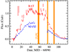 |
Fig. 1. Light curve of J0243 in the 2–20 and 15–50 keV energy bands obtained with the MAXI and Swift/BAT monitors, respectively. The vertical orange stripes show the times of IXPE observations. |
In this paper we present the results of IXPE observations of J0243 together with accompanying optical polarimetric observations. The details of the observations and their analysis are given in Sect. 2. Constraints on the pulsar geometry are worked through in Sect. 3. We discuss the results in Sect. 4. We conclude with a summary of our findings in Sect. 5.
2. Observations and data reduction
2.1. IXPE observations
The Imaging X-ray Polarimetry Explorer is a NASA mission in partnership with the Italian Space Agency (see a detailed description in Weisskopf et al. 2022), launched by a Falcon 9 rocket on 2021 December 9. There are three grazing incidence telescopes on board the observatory. Each telescope comprises an X-ray mirror assembly and a polarization-sensitive detector unit (DU) equipped with a gas-pixel detector (GPD; Soffitta et al. 2021; Baldini et al. 2021). These instruments provide imaging polarimetry in the 2–8 keV energy band with a time resolution better than 10 μs.
IXPE observed J0243 three times during 2023 July 20–August 25 (ObsID 02250799), on July 20–22, August 10–11, and August 23–25, with the total exposures of ≃168, 77, and 131 ks per telescope, respectively (see Fig. 1). We refer to these observations as Obs. 1, 2, and 3, respectively. The data were processed with the IXPEOBSSIM package version 31.0.1 (Baldini et al. 2022) using the CalDB version 20230702:v13. Source photons were collected in a circular region with a radius Rsrc = 70″ centered at the J0243 position. Because of the source brightness, the background was not subtracted following the recommendation by Di Marco et al. (2023). We performed the unweighted analysis (i.e., all events are taken into account independently of the quality of track reconstruction; Di Marco et al. 2022) of the IXPE data.
2.2. Timing
The event arrival times were corrected to the Solar System barycenter using the standard barycorr tool from the FTOOLS4 package (Blackburn 1995) and accounting for the effects of binary motion using the orbital parameters from the Fermi/GBM5 (see Table 1). The spin period (of P ≈ 9.79 s) and the spin period derivative were then determined for each IXPE observation segment using an epoch-folding search method, and then refined using phase-connection technique, which allows the phase of each event within a given segment to be unambiguously defined. The results are presented in Table 2. However, the gaps between the individual observation segments coupled to the complex evolution of intrinsic spin frequency and pulse profiles together with the remaining uncertainties in orbital parameters preclude the direct connection of phases between the segments.
Orbital parameters of J0243 from the Fermi/GBM data.
Timing parameters used to fold IXPE data.
The absolute phase alignment between the segments was therefore determined independently. Inspection of the pulse profile shape observed by IXPE (see bottom panel of Fig. 2) reveals some common features: the minimum around phase zero, several subpeaks within the main peak, and a peak around phase 0.9 appearing late in the outburst. The observed phases of these features can thus be used to determine absolute phase offset for each segment such that all peaks and dips (determined through the fitting of Gaussian functions) appear at the same pulse phase. The residual scatter can then be used to assess the remaining uncertainty in the final phase alignment, which we estimate to be below 1%. The phase alignment can also be checked through the comparison of the observed IXPE pulse profiles with hard X-ray pulse profiles observed by Fermi/GBM.
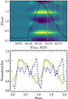 |
Fig. 2. Evolution of the pulse profiles during the outburst. Top: color-coded pulse profiles as observed by Fermi/GBM in units of relative intensities (see Appendix A.2 in Wilson-Hodge et al. 2018); yellow corresponds to the maxima of the pulse and dark blue to the minima. The black dashed line shows the evolution of the pulsed flux in the 12–50 keV range during the outburst as seen by Fermi/GBM (https://gammaray.nsstc.nasa.gov/gbm/science/pulsars/lightcurves/swiftj0243.html) with the peak flux being 4.8 × 10⁻⁹ erg cm−2 s−1. The shaded vertical stripes mark the times of IXPE observations. Bottom: normalized pulse profiles in the 2–8 keV band as observed by IXPE in three observations and shown with the solid orange, dotted green, and dashed blue lines for Obs. 1, 2, and 3, respectively. |
To this end, we used the enhanced products provided by the GBM team containing Fourier coefficients of the pulse profiles for a set of time intervals with typical duration of ∼3 d. These are expected to change smoothly, and since Fermi data contains no data gaps, the individual pulse profiles can be aligned through the cross-correlation of subsequent time intervals. The resulting pulse profile evolution is presented in the top panel of Fig. 2. We see that changes similar to those revealed by IXPE also occur in the GBM data: the secondary peak around phase 0.9 appears to be present only at lower luminosities and disappears at higher luminosities (i.e., our initial alignment using IXPE data alone proves to be robust).
2.3. Spectral analysis
For the spectral analysis, Stokes I spectra for Obs. 1, 2, and 3 were extracted using the xpbin tool’s PHA1 algorithm in IXPEOBBSIM, giving a set of three spectra (one for each DU) per observation. The energy spectra were binned to have at least 30 counts per energy channel. The spectra corresponding to the individual observations were fitted separately with the XSPEC package version 12.14.0 (Arnaud 1996) using χ2 statistics. The uncertainties are given at the 68.3% confidence level. Considering the energy resolution and energy range of IXPE, we used a simplified model consisting of an absorbed power law plus a blackbody component to fit the J0243 spectra. To account for the interstellar absorption, a multiplicative component tbabs with the abundances from Wilms et al. (2000) was applied. A re-normalization constant const was introduced to account for possible discrepancies between effective areas of the different DUs and was fixed at unity for DU1. The full spectral model is thus

The results of the spectral fitting are shown in Fig. 3, and the best-fit parameters are given in Table 3. We see that the fit quality is not good, which is caused partially by systematic errors in the instrument response and partially by the presence of a weak iron line around 6.5 keV. However, this does not preclude us from measuring the flux in the IXPE band. For calculations of the total luminosity we estimated the bolometric correction factor for our IXPE observations from the NuSTAR spectra at similar luminosities during the 2017 outburst (Tsygankov et al. 2018; Bykov et al. 2022). The maximum bolometric luminosity of the 2023 outburst is 1038 erg s−1, a factor of 20 lower than the peak of the 2017 outburst (see penultimate row of Table 3).
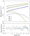 |
Fig. 3. IXPE spectra of J0243 in EFE representation. The red, green, and blue symbols and lines correspond to Obs. 1, 2, and 3, respectively. The solid, dashed, and dotted lines show the total model spectrum, the blackbody, and the power law, respectively. The bottom panel shows the fit residuals. |
Spectral parameters for the best-fit model obtained with XSPEC for Observations 1, 2, and 3.
We also studied variations in the spectrum over the pulse phase. Because the photon statistics do not allow us to use complex models, we fitted the phase-resolved spectra with a simple powerlaw model and fixed the hydrogen column density NH in the tbabs model at the best-fit phase-average values of 1.23, 1.01, and 1.56 × 1022 cm−2 for Obs. 1, 2, and 3, respectively. Variations in the best-fit photon index Γ with pulse phase are shown in Fig. 4b.
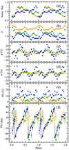 |
Fig. 4. Results from the pulse-phase-resolved analysis of J0243 in the 3–8 keV range, combining data from all DUs. Panel (a): pulse profile. Panel (b): photon spectral index. Panels (c) and (d): Dependence of the Stokes q and u parameters. Panels (e) and (f): PD and PA. The data from Obs. 1, 2, and 3 are shown as orange squares, green triangles, and blue circles, respectively. The typical error bar corresponding to 1σ uncertainty is shown in panels (c)–(e). The black solid curve is the best-fit RVM to the original PA data points (right column of Table 5). |
2.4. X-ray polarimetric analysis
The polarimetric parameters of J0243 were extracted utilizing the pcube algorithm (xpbin tool) in the IXPEOBSSIM package (Baldini et al. 2022), which follows the description of Kislat et al. (2015). We derived the normalized Stokes parameters q = Q/I and u = U/I, and subsequently the polarization degree PD= and polarization angle
  . The uncertainties are given at the 68.3% confidence level unless stated otherwise.
The data were divided into 24 separate pulse-phase bins. The polarization was found to be low in the 2–3 keV band. This motivated us to use for the following analysis only the 3–8 keV data to reduce the noise. The pulse-phase dependence of the normalized Stokes parameters q and u is displayed in Fig. 4c and d, and their evolution on the (q, u)-plane is shown in Fig. 5. The PD (shown in Fig. 4e) grows with time, from less than 8% in Obs. 1 to ∼12% in Obs. 2, and reaches a maximum of 24% in Obs. 3. The PA (Fig. 4f) has a double peak profile in all three observations. In Obs. 1 and 2 the amplitude of variations is about 100°6, while in Obs. 3 the data are consistent with two full revolution by 180° during the spin period. We do not see an obvious correlation between spectral shape and polarimetric properties.
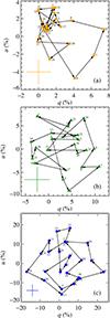 |
Fig. 5. Normalized Stokes parameters q and u for the phase-resolved polarimetric analysis using pcube (DUs combined), for the 3–8 keV energy band for Obs. 1 (panel a), 2 (panel b), and 3 (panel c). The typical error bar corresponding to 1σ uncertainty is shown in each panel. The phase bins are numbered. The scale in each panel is different. |
2.5. Optical polarization studies
The IXPE observations were accompanied by optical polarimetric observations in the R-band with the Robopol polarimeter located in the focal plane of the 1.3 m telescope of the Skinakas observatory (Greece). The observations were performed between 2023 July 28 and August 28 with multiple pointings. The data are presented in Table 4. We determined the intrinsic source polarization by subtracting the interstellar polarization using stars #1 and #2 (see Fig. 6), which are located ∼3′–4′ away from J0243 at a compatible distance of ∼5.7 kpc, as given by the Gaia EDR3 data (Bailer-Jones et al. 2021).
Optical polarization of J0243 as observed with Robopol in 2023 in R-band.
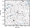 |
Fig. 6. Finding chart and the R-band polarization of J0243 (in the center) and three nearby field stars, which are situated at a similar distance according to Gaia parallaxes. The blue bars show the observed polarization of the source and field stars, while the red bar corresponds to the intrinsic polarization of the source from the Robopol observations, taking star #2 as an estimate of the interstellar contribution (see Table 4). |
We also analyzed optical polarimetric measurements of the source during its previous outburst in 2017 obtained with the Double-Image Polarimeter (DIPol-2; Piirola et al. 2014) at the T60 telescope at Haleakala, Hawaii (see Table A.1 in Appendix A). On average, 20 measurements of polarization were taken each night. We obtained the nightly averaged values using the 2σ clipping method (Kosenkov et al. 2017; Kosenkov 2021). To estimate the interstellar polarization, we also observed field star #3 (see Fig. 6), which was reasonably bright and also has a parallax similar to that of the source.
The resulting normalized Stokes parameters of J0243 and the field stars are shown in Fig. 7. The intrinsic optical PD lies between ∼1% and 2.5% and the intrinsic optical PA χo is in the range 20°–50°, depending on the choice of the field star.
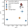 |
Fig. 7. Observed normalized Stokes parameters of the R-band optical polarization of J0243 and the three nearby field stars shown in Fig. 6. |
3. Pulsar geometry
3.1. RVM
Previous IXPE data on a number of X-ray pulsars (Doroshenko et al. 2022, 2023; Tsygankov et al. 2022, 2023; Mushtukov et al. 2023) were well described by the rotating vector model (RVM; Radhakrishnan & Cooke 1969; Meszaros et al. 1988). In this model, the evolution of the PA with pulsar phase is related to the projection of the magnetic dipole on the plane of the sky. If radiation is dominated by the ordinary-mode (O-mode) photons, the PA χ is given by Eq. (30) in Poutanen (2020):
Here χp is the position angle (measured from north to east) of the pulsar angular momentum, ip is the inclination of the pulsar spin with respect to the line of sight, θp is the magnetic obliquity (i.e., the angle between the magnetic dipole and the spin axis), and ϕp is the phase at which the northern magnetic pole passes in front of the observer (see Fig. 8 for geometry).
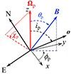 |
Fig. 8. Geometry of the pulsar and main parameters of the RVM. The pulsar angular momentum Ωp makes an angle ip with respect to the observer direction o. The angle θp is the magnetic obliquity, i.e., the angle between magnetic dipole and the rotation axis. The pulsar phase ϕ is the azimuthal angle of vector B in the plane (x, y) perpendicular to Ωp and ϕ = ϕp when B, Ωp, and o are coplanar. The pulsar position angle χp is the angle measured counterclockwise between the direction to the north (N) and the projection of Ωp on the plane of the sky (NE). |
If radiation is dominated by the extraordinary mode (X-mode), the PA is rotated by 90° with respect to the O-mode. The general relativistic effects are significant only if the NS rotates at millisecond periods (see Poutanen 2020; Loktev et al. 2020). The RVM is also theoretically justified, because the polarization vector of the radiation produced at the magnetic poles rotates adjusting to the magnetic field geometry until photons reach the adiabatic radius at a few tens of stellar radii due to the vacuum birefringence (Heyl et al. 2003), where the magnetic field is predominantly dipole (see Sect. 4.2).
We fit the RVM to a given set of Stokes parameters (q, u) as a function of pulsar phase. The PA distribution does not conform to a normal distribution, and hence we use the probability density function from Naghizadeh-Khouei & Clarke (1993),
![$$ \begin{aligned} G(\chi ) = \frac{1}{\sqrt{\pi }} \left\{ \frac{1}{\sqrt{\pi }} + \eta \mathrm{e}^{\eta ^2} \left[ 1 + \mathrm{erf}(\eta ) \right] \right\} \mathrm{e}^{-p_0^2/2} , \end{aligned} $$](/articles/aa/full_html/2024/11/aa50696-24/aa50696-24-eq5.gif)
where  is the measured PD in units of the error,
 ![$ \eta=p_0 \cos[2(\chi-\mathrm{PA})]/\sqrt{2} $](/articles/aa/full_html/2024/11/aa50696-24/aa50696-24-eq7.gif) , and erf is the error function. Here χ is the prediction of the RVM given by Eq. (2) for a given set of parameters and
, and erf is the error function. Here χ is the prediction of the RVM given by Eq. (2) for a given set of parameters and  . The best fit with the RVM to the pulse-phase dependent (q, u) is obtained by minimizing the log-likelihood function
with the sum taken over all phase bins k for a given observation i = 1, 2, 3 or summing over all of them. The error on a parameter can be obtained by varying that parameter and fitting all other parameters until Δlog L = 1 is reached. We can also, in principle, use a χ2 statistic to evaluate the quality of the fit. This is possible because for a highly significant detection of polarization, the PA is distributed almost normally, while the low-significance data points (when the PA distribution is far from normal) contribute very little to the χ2.
First, we fit the RVM to individual observations. The results are given in Table 5. We find that the best-fit parameters are vastly different, for example the pulsar inclination for the three observations is ip = 80°, 60°, and 33°. We note that the corresponding χ2 values for the best fits are 25.1, 83.3, and 65.7 for 20 degrees of freedom (d.o.f.) for Obs. 1–3, respectively. Thus, only the fit to Obs. 1 is reasonably good. If, on the other hand, we force the RVM parameters to be the same, we get the best-fit parameters of ip = 47°, θp = 83°, χp = −67°, and ϕp = 0.64 (this RVM is shown in Fig. 4f), but an unacceptable fit with χ2/d.o.f. = 276/68. Thus, we find that the RVM does not provide a good description of the data.
Best-fit RVM parameters for the three IXPE observations.
A similar situation occurred with the brightest transient pulsar observed by IXPE, LS V +44 17/RX J0440.9+4431, which showed the peak luminosity of 4.3 × 1037 erg s−1 during its giant outburst in 2023 January–February (Salganik et al. 2023). In this object, significant changes in the RVM parameters were detected (Doroshenko et al. 2023). There, the pulse-phase resolved Stokes q and u parameters for two epochs of observations traced similar patterns on the (q, u) plane, but the figures were shifted relative to each other (see Poutanen et al. 2024). An additional, phase-independent polarized component was introduced to align the results with the RVM predictions. We now apply the same idea to the J0243 data.
3.2. Two-component polarization model
Similarly to Doroshenko et al. (2023), we assume that there are two polarized components in the J0243 data. The first is associated with the pulsar and is described by the RVM. The second component is independent of the pulsar phase. We express the absolute Stokes parameters for each observation as a sum of the variable and constant components:
![$$ \begin{aligned} I(\phi )&= I_{\rm c} + I_{\rm p}(\phi ) , \nonumber \\ Q(\phi )&= Q_{\rm c} + P_{\rm p}(\phi )I_{\rm p}(\phi )\cos [2\chi (\phi )] , \\ U(\phi )&= U_{\rm c} + P_{\rm p}(\phi )I_{\rm p}(\phi ) \sin [2\chi (\phi )] . \nonumber \end{aligned} $$](/articles/aa/full_html/2024/11/aa50696-24/aa50696-24-eq13.gif)
Here we consider the observed Stokes parameters I, Q, and U to be scaled to the average flux value with indices denoting the constant (c) and pulsed (p) components. The PD of the variable component is Pp and its PA χ is given by Eq. (2). The scaled Stokes parameters of the constant component (Qc, Uc) are related to the PD, Pc, and the flux, Ic, as

with its PA being  .
.
We assume that the pulsar geometry (i.e., RVM parameters) does not change between the observations and the observed changes in the polarization properties are related to the presence of an additional unpulsed polarized component. In order to describe the data from all three observations, in addition to the four RVM parameters, we introduce six additional free parameters Qc, i and Uc, i, i = 1, 2, 3, which describe properties of this constant component. For a given set of Qc, i and Uc, i, we can construct the differences Qp = Q(ϕ)−Qc, Up = U(ϕ)−Uc, which are fit by the RVM using maximum likelihood function with the probabilities given by Eq. (3). The best-fit RVM parameters as well as the Stokes parameters of the constant component are given in the top part of Table 6. The quality of the fit is much better than with the RVM model alone. The Akaike information criterion (AIC; Akaike 1974) decreases by Δ AIC = 21.5, implying that the pure RVM model is exp(Δ AIC/2) = 4.7 × 10⁴ less probable that the two-component model.
Best-fit parameters of the two-component model.
The obtained Stokes parameters of the constant component correspond to the polarized fluxes (in units of the average flux) of  in the range ∼1–4%. Once the best-fit parameters of the constant component are determined, we can obtain the value of the PA for the variable component using Eq. (5):
![$$ \begin{aligned} \chi (\phi ) = \frac{1}{2} \arctan \left[ \frac{U(\phi )-U_{\rm c}}{Q(\phi )-Q_{\rm c}}\right] . \end{aligned} $$](/articles/aa/full_html/2024/11/aa50696-24/aa50696-24-eq26.gif)
We found that the PA values of the constant component χc, i for the three observations are the same within the errors. This motivated us to perform another fit with the fixed χc for all three observations (which reduced the number of free parameters by 2). We refitted the data by varying, in addition to the four RVM parameters, three polarized fluxes Pc, iIc, i and the PA χc. The best-fit parameters are presented in the bottom part of Table 6. We see that the quality of the fit is not getting much worse, with Δ AIC = 2.3, which means that the model is three times less probable. The PA of the varying component associated with the pulsar as obtained using Eq. (7) are plotted in Fig. 9 together with the best-fit RVM. In order to obtain the covariance plot for these model parameters we used the affine invariant Markov chain Monte Carlo ensemble sampler EMCEE package of PYTHON (Foreman-Mackey et al. 2013). The resulting posterior distributions are shown in Fig. 10.
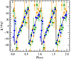 |
Fig. 9. Pulse-phase dependence of the PA of the variable (pulsar) components after subtracting the best-fit constant polarized component from the observed Stokes parameters. The orange squares, green triangles, and blue circles with error bars correspond to Obs. 1, 2, and 3, respectively. The black line is the best-fit RVM from the two-component model (see lower part of Table 6) to all three data sets. |
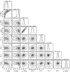 |
Fig. 10. Corner plot of the posterior distribution for parameters of the RVM plus a constant model with one free PA given by Eqs. (5) fitted directly to the (q, u) values using likelihood function (3). Here PFi, i = 1, 2, and 3 is the polarized flux PcIc of the constant component (measured in units of the average flux) during Obs. 1, 2, and 3, respectively, and χc is its polarization angle. The two-dimensional contours correspond to 68.3%, 95.45%, and 99.73% confidence levels. The histograms show the normalized one-dimensional distributions for a given parameter derived from the posterior samples. |
4. Discussion
4.1. System geometry and origin of constant polarized component
Our fits demonstrated that polarization cannot be described with a simple RVM. The main reason is that while the PA makes two full turns (by 180°) during one pulsar period during Obs. 3, it shows a double sine wave during Obs. 1 and 2. This behavior contradicts the RVM. Furthermore, the quality of the fit is rather bad and the best-fit pulsar geometrical parameters vary strongly between observations (see Table 5).
Following Doroshenko et al. (2023), in addition to the direct pulsar radiation described by the RVM, we assumed that there is a pulse-phase-independent polarized component. The data are much better described by this two-component model with a constant set of RVM parameters. The PA of the constant component in the three observations was found to lie between −20° and 14°, consistent with being the same within the errors. Fixing this PA at the same value gave the best-fit value of χc = 8° ±7°. We found that the polarized flux (in units of the average flux) of the constant component PcIc is between 1.5% and 3%. Because the contribution of this component to the total flux is unknown, the value of Pc is not well determined. The lower limit on Pc comes from the fact that the flux of the constant component cannot exceed the flux minimum of around 60% of the average flux (see Fig. 2). This results in Pc ≳ 3.5–5% depending on the observation, with the value growing inversely proportional to Ic. A lower limit on Ic comes from the condition Pc < 100%, which translates to Ic ≳ 1.5–3%. If we assume more realistically that Pc ≲ 30% (see below), then Ic ≳ 5–10%.
The constant component can be associated with scattering in the equatorial accretion disk wind (Doroshenko et al. 2023). If the wind half-opening angle is 30°, it occupies half of the sky as seen from the central source. Thus, for the Thomson optical depth through the wind of 0.2, about 10% of pulsar radiation is scattered by the wind. The PD of the scattered component depends on the disk inclination as ≈sin2id/(3 − cos2id) (Sunyaev & Titarchuk 1985; Nitindala et al., in prep.). For id > 60°, the PD is close to 30% and the polarized flux in that case has to be around 3% of the average flux consistent with the data. At lower id, a larger contribution of this component to the average flux is required.
The PA of the constant X-ray component is ∼10° (or −170°). If its polarization is produced in the accretion disk wind, it is natural to assume that the PA is related to the position angle of the accretion disk axis. On the other hand, polarization in the optical band is likely produced by scattering of the Be-star radiation off the decretion disk (which occupies a much larger solid angle than the accretion disk around a NS), and therefore provides the orientation of that disk. Because of the uncertainty in the value of the IS polarization, the intrinsic optical PA χo is in the range between 20° and 50° (see Tables 4 and A.1). The lowest value of χo (corresponding to the closest star #1 as a proxy for IS polarization) is within 2σ of χc, while the highest PA is clearly inconsistent with that. Thus, there is an indication that the accretion and decretion disks are somewhat misaligned.
From the two-component model fit, we constrained the pulsar inclination at ip ≈ 15°–40° and the magnetic obliquity to θp ≈ 60°–80°. The pulsar rotation axis position angle is χp ≈ −50° ±10°, which is clearly inconsistent with the PA of the constant component χc. If pulsar radiation escapes in the X-mode, then χp ≈ 40° (or −140°), which is still far from χc. Under the assumption that χc gives the orientation of the accretion disk (and the binary orbit), the difference |χp − χc| is related to the misalignment angle between the pulsar spin axis and the orbital axis, which is then about 30°–50°.
We note that evidence for a misalignment was also found in other pulsars. For example, in LS V +44 17 (Doroshenko et al. 2023) we found χo ≈ χc ∼ 60° −70°, and both were inconsistent with χp ≈ −10° implying a misalignment of ∼75° if the pulsar emits predominantly in the O-mode or at least 15° for emission in the X-mode. In Her X-1 (Doroshenko et al. 2022; Heyl et al. 2024), the misalignment is at least 25°, but can be ∼65° or even higher.
Finally, we note that the quality of the fit with the two-component model is still not statistically acceptable, likely indicating that the actual physical situation is even more complex. The polarization properties of the additional component may vary with the pulsar phase somehow, but not with the amplitude comparable to that of the pulsar itself. For example, scattering in the wind can be phase-dependent because of the azimuthal asymmetry of the pulsar radiation.
4.2. Polarization–flux anti-correlation
Our fits demonstrate that most of the polarized flux is produced by the pulsating component. Furthermore, the observed polarization has a clear trend of increasing PD with decreasing flux. We wondered what the most probable reason for such a behavior could be.
At low luminosities when most of the radiation is produced in two small hotspots at the NS surface close to the magnetic poles, the PD is determined by the structure of the atmosphere and the energy dissipation profile (Doroshenko et al. 2022). The PD is conserved when photons propagate through the magnetosphere and the polarization vector adjusts to the orientation of the magnetic field until the adiabatic radius is reached (e.g., Heyl & Shaviv 2002; Taverna et al. 2015). The adiabatic radius as a function of photon energy E is (Heyl & Caiazzo 2018; Taverna & Turolla 2024)
where B13 is the surface magnetic field strength in units of 1013 G, and R6 is the NS radius in units of 106 cm. For the surface magnetic field of B13 ≈ 1 (Kong et al. 2022) and R6 ≈ 1.2 (e.g., Nättilä et al. 2017; Miller et al. 2020; Annala et al. 2022), it exceeds the NS radius for photons in the IXPE range by more than an order of magnitude. At this distance, the magnetic field is mostly dipole resulting in the PA that follows the RVM, as indeed observed in a number of X-ray pulsars (Doroshenko et al. 2022; Malacaria et al. 2023; Tsygankov et al. 2023; Suleimanov et al. 2023; Mushtukov et al. 2023; Heyl et al. 2024).
At a luminosity close to 1038 erg s−1, a number of additional effects come into play. First, the emission region is not point-like anymore, but radiation is produced in an accretion column, which stands above the NS surface. Locally, the polarization direction correlates with the magnetic field direction. However, the PD of the whole column radiation can be smaller that the local values, because of the different energy dissipation profile, varying depth of the vacuum resonance (Gnedin et al. 1978), and resulting mode conversions (Pavlov & Shibanov 1979; Lai & Ho 2003; Doroshenko et al. 2022; Lai 2023). Second, a substantial part of the column radiation illuminates the NS surface and is reflected from that (Lyubarskii & Syunyaev 1988; Poutanen et al. 2013). Because of the different relative contributions of the O- and X-modes in the reflected radiation, the total PD is reduced. Finally, the accretion flow is expected to be optically thick (Mushtukov et al. 2017, 2019) within the NS magnetospheric radius

where Λ is coefficient typically taken to be ∼0.5 for the case of disk accretion (Chashkina et al. 2019),  is the mass accretion rate in units of 1018 g s−1, and m ≈ 1.5 is the mass of a NS in solar masses. Under this condition, a substantial fraction of X-ray photons emitted close the NS surface is reprocessed by the optically thick envelope created around the NS magnetospheric cavities. Because the size of the magnetosphere exceeds the adiabatic radius, the final polarization of X-ray photons is defined by scattering off the envelope. The PD and PA depend more on the scattering geometry than on the projection of the NS magnetic dipole on the sky. Integrating the Stokes parameters over the envelope significantly reduces the total PD. Thus, in this model the observed anticorrelation of the PD and flux is a result of variable optical thickness of the envelope: the higher the mass accretion rate and the flux, the larger the optical thickness of envelope, and thus the larger the fraction of photons experiencing reprocessing by the envelope outside the NS adiabatic radius that reduces the PD.
5. Summary
Swift J0243.6+6124 was observed by IXPE in 2023 July–August three times during its outburst. The main results of our study of its polarimetric properties can be summarized as follows:
-
Using updated pulsar ephemeris from Fermi/GBM we were able to phase connect the pulse arrival times for the whole duration of the outburst.
-
The phase-resolved polarimetric analysis revealed a significant detection of X-ray polarization with the PD reaching ∼6%, 10%, and 20% during the three observations separated by a month when the flux dropped by a factor of three.
-
We showed that evolution of the PA with pulsar phase in Obs. 1 and 2 having a double sine wave structure is inconsistent with the RVM. This brought us to the conclusion that the likely reason for this discrepancy is the presence of the phase-independent polarized component produced, for example by scattering in the accretion disk wind, as was proposed for another bright X-ray pulsar LS V +44 17 (Doroshenko et al. 2023; Poutanen et al. 2024).
-
Assuming the same RVM parameters for the three observations, we fitted the data with the two-component model and obtained the PA of the constant component χc between −20° and 15°. Assuming that the PA for all observations is the same, we find χc = 8° ±7°. Also assuming that the constant component contributes 10% of the average flux, we find that the PD of that component varies between 15% and 30%. We estimated the inclination of the NS rotation axis to the line of sight of ip = 15°–40°, the magnetic obliquity of θp = 60°–80°, and the pulsar position angle of χp ≈ −50°.
-
Using optical polarimetric observations of the source and nearby field stars, we determined that the intrinsic PA χo lies between 20° and 50°, depending on the choice of field star to estimate the contribution of the interstellar component. The lowest value of χo is consistent with χc within 2σ, while the higher PA are clearly inconsistent with that value. Associating optical polarization with scattering in the decretion disk, the data indicate a possible misalignment between accretion and decretion disks axes.
-
A deviation of χc from the pulsar position angle χp implies a ≳30° misalignment between pulsar rotation axis and the orbital (accretion disk) axis.
This is closer than the distance of 6.8 kpc from the Gaia DR2 catalog (Bailer-Jones et al. 2018) and used in some earlier literature.
This is in strong disagreement with the recent analysis of Obs. 1 by Majumder et al. (2024), who used only five phase bins.
Acknowledgments
The Imaging X-ray Polarimetry Explorer (IXPE) is a joint US and Italian mission. The US contribution is supported by the National Aeronautics and Space Administration (NASA) and led and managed by its Marshall Space Flight Center (MSFC), with industry partner Ball Aerospace (contract NNM15AA18C). The Italian contribution is supported by the Italian Space Agency (Agenzia Spaziale Italiana, ASI) through contract ASI-OHBI-2022-13-I.0, agreements ASI-INAF-2022-19-HH.0 and ASI-INFN-2017.13-H0, and its Space Science Data Center (SSDC) with agreements ASI-INAF-2022-14-HH.0 and ASI-INFN 2021-43-HH.0, and by the Istituto Nazionale di Astrofisica (INAF) and the Istituto Nazionale di Fisica Nucleare (INFN) in Italy. This research used data products provided by the IXPE Team (MSFC, SSDC, INAF, and INFN) and distributed with additional software tools by the High-Energy Astrophysics Science Archive Research Center (HEASARC), at NASA Goddard Space Flight Center (GSFC). This research has been supported by the Academy of Finland grants 333112, 349144 and 355672 (JP, SST, AV), the German Academic Exchange Service (DAAD) travel grant 57525212 (VD, VFS), UKRI Stephen Hawking fellowship (AAM), Finnish Cultural Foundation grant (VKra), Natural Sciences and Engineering Research Council of Canada (JH), and Deutsche Forschungsgemeinschaft (DFG) grant WE 1312/59-1 (VFS). IL was supported by the NASA Postdoctoral Program at the Marshall Space Flight Center, administered by Oak Ridge Associated Universities under contract with NASA. Nordita is supported in part by NordForsk.
References
- Akaike, H. 1974, IEEE Trans. Auto. Control, 19, 716 [Google Scholar]
- Annala, E., Gorda, T., Katerini, E., et al. 2022, Phys. Rev. X, 12, 011058 [NASA ADS] [Google Scholar]
- Arnaud, K. A. 1996, ASP Conf. Ser., 101, 17 [Google Scholar]
- Bachetti, M., Harrison, F. A., Walton, D. J., et al. 2014, Nature, 514, 202 [NASA ADS] [CrossRef] [Google Scholar]
- Bailer-Jones, C. A. L., Rybizki, J., Fouesneau, M., Mantelet, G., & Andrae, R. 2018, AJ, 156, 58 [Google Scholar]
- Bailer-Jones, C. A. L., Rybizki, J., Fouesneau, M., Demleitner, M., & Andrae, R. 2021, AJ, 161, 147 [Google Scholar]
- Baldini, L., Barbanera, M., Bellazzini, R., et al. 2021, Astropart. Phys., 133, 102628 [NASA ADS] [CrossRef] [Google Scholar]
- Baldini, L., Bucciantini, N., Lalla, N. D., et al. 2022, SoftwareX, 19, 101194 [NASA ADS] [CrossRef] [Google Scholar]
- Basko, M. M., & Sunyaev, R. A. 1976, MNRAS, 175, 395 [Google Scholar]
- Bikmaev, I., Shimansky, V., Irtuganov, E., et al. 2017, ATel, 10968, 1 [Google Scholar]
- Blackburn, J. K. 1995, ASP Conf. Ser., 77, 367 [NASA ADS] [Google Scholar]
- Brice, N., Zane, S., Turolla, R., & Wu, K. 2021, MNRAS, 504, 701 [NASA ADS] [CrossRef] [Google Scholar]
- Bykov, S. D., Gilfanov, M. R., Tsygankov, S. S., & Filippova, E. V. 2022, MNRAS, 516, 1601 [NASA ADS] [CrossRef] [Google Scholar]
- Carpano, S., Haberl, F., Maitra, C., & Vasilopoulos, G. 2018, MNRAS, 476, L45 [NASA ADS] [CrossRef] [Google Scholar]
- Cenko, S. B., Barthelmy, S. D., D’Avanzo, P., et al. 2017, GRB Coordinates Network, 21960, 1 [NASA ADS] [Google Scholar]
- Chashkina, A., Lipunova, G., Abolmasov, P., & Poutanen, J. 2019, A&A, 626, A18 [NASA ADS] [CrossRef] [EDP Sciences] [Google Scholar]
- Di Marco, A., Costa, E., Muleri, F., et al. 2022, AJ, 163, 170 [NASA ADS] [CrossRef] [Google Scholar]
- Di Marco, A., Soffitta, P., Costa, E., et al. 2023, AJ, 165, 143 [CrossRef] [Google Scholar]
- Doroshenko, V., Tsygankov, S., & Santangelo, A. 2018, A&A, 613, A19 [NASA ADS] [CrossRef] [EDP Sciences] [Google Scholar]
- Doroshenko, V., Poutanen, J., Tsygankov, S. S., et al. 2022, Nat. Astron., 6, 1433 [NASA ADS] [CrossRef] [Google Scholar]
- Doroshenko, V., Poutanen, J., Heyl, J., et al. 2023, A&A, 677, A57 [NASA ADS] [CrossRef] [EDP Sciences] [Google Scholar]
- Foreman-Mackey, D., Hogg, D. W., Lang, D., & Goodman, J. 2013, PASP, 125, 306 [Google Scholar]
- Forsblom, S. V., Poutanen, J., Tsygankov, S. S., et al. 2023, ApJ, 947, L20 [NASA ADS] [CrossRef] [Google Scholar]
- Forsblom, S. V., Tsygankov, S. S., Poutanen, J., et al. 2024, A&A, in press, https://doi.org/10.1051/0004-6361/202450937 [Google Scholar]
- Fürst, F., Walton, D. J., Harrison, F. A., et al. 2016, ApJ, 831, L14 [Google Scholar]
- Gehrels, N., Chincarini, G., Giommi, P., et al. 2004, ApJ, 611, 1005 [Google Scholar]
- Gnedin, Y. N., Pavlov, G. G., & Shibanov, Y. A. 1978, Sov. Astron. Lett., 4, 117 [Google Scholar]
- Heyl, J., & Caiazzo, I. 2018, Galaxies, 6, 76 [NASA ADS] [CrossRef] [Google Scholar]
- Heyl, J. S., & Shaviv, N. J. 2002, Phys. Rev. D, 66, 023002 [NASA ADS] [CrossRef] [Google Scholar]
- Heyl, J. S., Shaviv, N. J., & Lloyd, D. 2003, MNRAS, 342, 134 [NASA ADS] [CrossRef] [Google Scholar]
- Heyl, J., Doroshenko, V., González-Caniulef, D., et al. 2024, Nat. Astron., 8, 1047 [NASA ADS] [CrossRef] [Google Scholar]
- Israel, G. L., Belfiore, A., Stella, L., et al. 2017, Science, 355, 817 [NASA ADS] [CrossRef] [Google Scholar]
- Kaaret, P., Feng, H., & Roberts, T. P. 2017, ARA&A, 55, 303 [Google Scholar]
- Kennea, J. A., Lien, A. Y., Krimm, H. A., Cenko, S. B., & Siegel, M. H. 2017, ATel, 10809, 1 [Google Scholar]
- Kennea, J. A., Bahramian, A., & Negoro, H. 2023, ATel, 15984, 1 [NASA ADS] [Google Scholar]
- King, A., Lasota, J.-P., & Middleton, M. 2023, New Astron. Rev., 96, 101672 [CrossRef] [Google Scholar]
- King, A. R., Davies, M. B., Ward, M. J., Fabbiano, G., & Elvis, M. 2001, ApJ, 552, L109 [NASA ADS] [CrossRef] [Google Scholar]
- Kislat, F., Clark, B., Beilicke, M., & Krawczynski, H. 2015, Astropart. Phys., 68, 45 [NASA ADS] [CrossRef] [Google Scholar]
- Kong, L.-D., Zhang, S., Zhang, S.-N., et al. 2022, ApJ, 933, L3 [NASA ADS] [CrossRef] [Google Scholar]
- Kosenkov, I. A. 2021, Dipol2Red: Linear Polarization Data Reduction Pipeline for DIPol-2 and DIPol-UF Polarimeters [Google Scholar]
- Kosenkov, I. A., Berdyugin, A. V., Piirola, V., et al. 2017, MNRAS, 468, 4362 [NASA ADS] [CrossRef] [Google Scholar]
- Kouroubatzakis, K., Reig, P., Andrews, J., & Zezas, A. 2017, ATel, 10822, 1 [Google Scholar]
- Lai, D. 2023, PNAS, 120, e2216534120 [NASA ADS] [CrossRef] [Google Scholar]
- Lai, D., & Ho, W. C. G. 2003, ApJ, 588, 962 [NASA ADS] [CrossRef] [Google Scholar]
- Lipunov, V. M. 1982, Sov. Astron., 26, 54 [Google Scholar]
- Loktev, V., Salmi, T., Nättilä, J., & Poutanen, J. 2020, A&A, 643, A84 [NASA ADS] [CrossRef] [EDP Sciences] [Google Scholar]
- Lyubarskii, Y. E., & Syunyaev, R. A. 1988, Sov. Astron. Lett., 14, 390 [NASA ADS] [Google Scholar]
- Majumder, S., Chatterjee, R., Jayasurya, K. M., Das, S., & Nandi, A. 2024, ApJ, 971, L21 [NASA ADS] [CrossRef] [Google Scholar]
- Malacaria, C., Heyl, J., Doroshenko, V., et al. 2023, A&A, 675, A29 [NASA ADS] [CrossRef] [EDP Sciences] [Google Scholar]
- Marin, F., Marinucci, A., Laurenti, M., et al. 2024, A&A, 689, A238 [NASA ADS] [CrossRef] [EDP Sciences] [Google Scholar]
- Matsuoka, M., Kawasaki, K., Ueno, S., et al. 2009, PASJ, 61, 999 [Google Scholar]
- Matt, G. 1993, MNRAS, 260, 663 [NASA ADS] [CrossRef] [Google Scholar]
- Meszaros, P., Novick, R., Szentgyorgyi, A., Chanan, G. A., & Weisskopf, M. C. 1988, ApJ, 324, 1056 [NASA ADS] [CrossRef] [Google Scholar]
- Miller, M. C., Chirenti, C., & Lamb, F. K. 2020, ApJ, 888, 12 [Google Scholar]
- Mushtukov, A. A., & Portegies Zwart, S. 2023, MNRAS, 518, 5457 [Google Scholar]
- Mushtukov, A. A., Suleimanov, V. F., Tsygankov, S. S., & Poutanen, J. 2015, MNRAS, 447, 1847 [NASA ADS] [CrossRef] [Google Scholar]
- Mushtukov, A. A., Suleimanov, V. F., Tsygankov, S. S., & Ingram, A. 2017, MNRAS, 467, 1202 [NASA ADS] [Google Scholar]
- Mushtukov, A. A., Ingram, A., Middleton, M., Nagirner, D. I., & van der Klis, M. 2019, MNRAS, 484, 687 [NASA ADS] [CrossRef] [Google Scholar]
- Mushtukov, A. A., Portegies Zwart, S., Tsygankov, S. S., Nagirner, D. I., & Poutanen, J. 2021, MNRAS, 501, 2424 [NASA ADS] [CrossRef] [Google Scholar]
- Mushtukov, A. A., Tsygankov, S. S., Poutanen, J., et al. 2023, MNRAS, 524, 2004 [NASA ADS] [CrossRef] [Google Scholar]
- Naghizadeh-Khouei, J., & Clarke, D. 1993, A&A, 274, 968 [NASA ADS] [Google Scholar]
- Nättilä, J., Miller, M. C., Steiner, A. W., et al. 2017, A&A, 608, A31 [NASA ADS] [CrossRef] [EDP Sciences] [Google Scholar]
- Ng, M., Sanna, A., Chakrabarty, D., et al. 2023, ATel, 15987, 1 [NASA ADS] [Google Scholar]
- Pavlov, G. G., & Shibanov, Y. A. 1979, JETP, 49, 741 [NASA ADS] [Google Scholar]
- Piirola, V., Berdyugin, A., & Berdyugina, S. 2014, Proc. SPIE, 9147, 91478I [NASA ADS] [Google Scholar]
- Poutanen, J. 2020, A&A, 641, A166 [NASA ADS] [CrossRef] [EDP Sciences] [Google Scholar]
- Poutanen, J., Nagendra, K. N., & Svensson, R. 1996, MNRAS, 283, 892 [NASA ADS] [CrossRef] [Google Scholar]
- Poutanen, J., Lipunova, G., Fabrika, S., Butkevich, A. G., & Abolmasov, P. 2007, MNRAS, 377, 1187 [NASA ADS] [CrossRef] [Google Scholar]
- Poutanen, J., Mushtukov, A. A., Suleimanov, V. F., et al. 2013, ApJ, 777, 115 [NASA ADS] [CrossRef] [Google Scholar]
- Poutanen, J., Tsygankov, S. S., & Forsblom, S. V. 2024, Galaxies, 12, 46 [NASA ADS] [CrossRef] [Google Scholar]
- Radhakrishnan, V., & Cooke, D. J. 1969, Astrophys. Lett., 3, 225 [NASA ADS] [Google Scholar]
- Rodríguez Castillo, G. A. 2020, ApJ, 895, 60 [CrossRef] [Google Scholar]
- Salganik, A., Tsygankov, S. S., Doroshenko, V., et al. 2023, MNRAS, 524, 5213 [NASA ADS] [CrossRef] [Google Scholar]
- Setoguchi, K., Negoro, H., Nakajima, M., et al. 2023, ATel, 15983, 1 [NASA ADS] [Google Scholar]
- Soffitta, P., Baldini, L., Bellazzini, R., et al. 2021, AJ, 162, 208 [CrossRef] [Google Scholar]
- Suleimanov, V. F., Forsblom, S. V., Tsygankov, S. S., et al. 2023, A&A, 678, A119 [NASA ADS] [CrossRef] [EDP Sciences] [Google Scholar]
- Sunyaev, R. A., & Titarchuk, L. G. 1985, A&A, 143, 374 [NASA ADS] [Google Scholar]
- Taverna, R., & Turolla, R. 2024, Galaxies, 12, 6 [NASA ADS] [CrossRef] [Google Scholar]
- Taverna, R., Turolla, R., Gonzalez Caniulef, D., et al. 2015, MNRAS, 454, 3254 [NASA ADS] [CrossRef] [Google Scholar]
- Tsygankov, S. S., Doroshenko, V., Mushtukov, A. A., Lutovinov, A. A., & Poutanen, J. 2018, MNRAS, 479, L134 [CrossRef] [Google Scholar]
- Tsygankov, S. S., Doroshenko, V., Poutanen, J., et al. 2022, ApJ, 941, L14 [NASA ADS] [CrossRef] [Google Scholar]
- Tsygankov, S. S., Doroshenko, V., Mushtukov, A. A., et al. 2023, A&A, A48 [NASA ADS] [CrossRef] [EDP Sciences] [Google Scholar]
- Ursini, F., Marinucci, A., Matt, G., et al. 2023, MNRAS, 519, 50 [Google Scholar]
- Veledina, A., Muleri, F., Poutanen, J., et al. 2024, Nat. Astron., 8, 1031 [NASA ADS] [CrossRef] [Google Scholar]
- Weisskopf, M. C., Soffitta, P., Baldini, L., et al. 2022, JATIS, 8, 026002 [NASA ADS] [Google Scholar]
- Wilms, J., Allen, A., & McCray, R. 2000, ApJ, 542, 914 [Google Scholar]
- Wilson-Hodge, C. A., Malacaria, C., Jenke, P. A., et al. 2018, ApJ, 863, 9 [Google Scholar]
- Xiao, Y. X., Xu, Y. J., Ge, M. Y., et al. 2024, ApJ, 965, 18 [NASA ADS] [CrossRef] [Google Scholar]
- Zel’dovich, Y. B., & Shakura, N. I. 1969, Sov. Astron., 13, 175 [NASA ADS] [Google Scholar]
Appendix A: Optical polarimetric observations during 2017 outburst
Table A.1 presents the results of the optical polarimetric measurements of J0243 during its 2017 outburst obtained with DIPol-2 (Piirola et al. 2014) at the T60 telescope at Haleakala, Hawaii. Polarization of the field star #3 (see Fig. 6) was determined using observations in February 2024 at the same telescope.
Optical polarization of J0243 as observed with DIPol-2 in three filters B, V, and R in 2017.
All Tables
Spectral parameters for the best-fit model obtained with XSPEC for Observations 1, 2, and 3.
Optical polarization of J0243 as observed with DIPol-2 in three filters B, V, and R in 2017.
All Figures
|
Fig. 1. Light curve of J0243 in the 2–20 and 15–50 keV energy bands obtained with the MAXI and Swift/BAT monitors, respectively. The vertical orange stripes show the times of IXPE observations. |
| In the text | |
|
Fig. 2. Evolution of the pulse profiles during the outburst. Top: color-coded pulse profiles as observed by Fermi/GBM in units of relative intensities (see Appendix A.2 in Wilson-Hodge et al. 2018); yellow corresponds to the maxima of the pulse and dark blue to the minima. The black dashed line shows the evolution of the pulsed flux in the 12–50 keV range during the outburst as seen by Fermi/GBM (https://gammaray.nsstc.nasa.gov/gbm/science/pulsars/lightcurves/swiftj0243.html) with the peak flux being 4.8 × 10⁻⁹ erg cm−2 s−1. The shaded vertical stripes mark the times of IXPE observations. Bottom: normalized pulse profiles in the 2–8 keV band as observed by IXPE in three observations and shown with the solid orange, dotted green, and dashed blue lines for Obs. 1, 2, and 3, respectively. |
| In the text | |
|
Fig. 3. IXPE spectra of J0243 in EFE representation. The red, green, and blue symbols and lines correspond to Obs. 1, 2, and 3, respectively. The solid, dashed, and dotted lines show the total model spectrum, the blackbody, and the power law, respectively. The bottom panel shows the fit residuals. |
| In the text | |
|
Fig. 4. Results from the pulse-phase-resolved analysis of J0243 in the 3–8 keV range, combining data from all DUs. Panel (a): pulse profile. Panel (b): photon spectral index. Panels (c) and (d): Dependence of the Stokes q and u parameters. Panels (e) and (f): PD and PA. The data from Obs. 1, 2, and 3 are shown as orange squares, green triangles, and blue circles, respectively. The typical error bar corresponding to 1σ uncertainty is shown in panels (c)–(e). The black solid curve is the best-fit RVM to the original PA data points (right column of Table 5). |
| In the text | |
|
Fig. 5. Normalized Stokes parameters q and u for the phase-resolved polarimetric analysis using pcube (DUs combined), for the 3–8 keV energy band for Obs. 1 (panel a), 2 (panel b), and 3 (panel c). The typical error bar corresponding to 1σ uncertainty is shown in each panel. The phase bins are numbered. The scale in each panel is different. |
| In the text | |
|
Fig. 6. Finding chart and the R-band polarization of J0243 (in the center) and three nearby field stars, which are situated at a similar distance according to Gaia parallaxes. The blue bars show the observed polarization of the source and field stars, while the red bar corresponds to the intrinsic polarization of the source from the Robopol observations, taking star #2 as an estimate of the interstellar contribution (see Table 4). |
| In the text | |
|
Fig. 7. Observed normalized Stokes parameters of the R-band optical polarization of J0243 and the three nearby field stars shown in Fig. 6. |
| In the text | |
|
Fig. 8. Geometry of the pulsar and main parameters of the RVM. The pulsar angular momentum Ωp makes an angle ip with respect to the observer direction o. The angle θp is the magnetic obliquity, i.e., the angle between magnetic dipole and the rotation axis. The pulsar phase ϕ is the azimuthal angle of vector B in the plane (x, y) perpendicular to Ωp and ϕ = ϕp when B, Ωp, and o are coplanar. The pulsar position angle χp is the angle measured counterclockwise between the direction to the north (N) and the projection of Ωp on the plane of the sky (NE). |
| In the text | |
|
Fig. 9. Pulse-phase dependence of the PA of the variable (pulsar) components after subtracting the best-fit constant polarized component from the observed Stokes parameters. The orange squares, green triangles, and blue circles with error bars correspond to Obs. 1, 2, and 3, respectively. The black line is the best-fit RVM from the two-component model (see lower part of Table 6) to all three data sets. |
| In the text | |
|
Fig. 10. Corner plot of the posterior distribution for parameters of the RVM plus a constant model with one free PA given by Eqs. (5) fitted directly to the (q, u) values using likelihood function (3). Here PFi, i = 1, 2, and 3 is the polarized flux PcIc of the constant component (measured in units of the average flux) during Obs. 1, 2, and 3, respectively, and χc is its polarization angle. The two-dimensional contours correspond to 68.3%, 95.45%, and 99.73% confidence levels. The histograms show the normalized one-dimensional distributions for a given parameter derived from the posterior samples. |
| In the text | |
Current usage metrics show cumulative count of Article Views (full-text article views including HTML views, PDF and ePub downloads, according to the available data) and Abstracts Views on Vision4Press platform.
Data correspond to usage on the plateform after 2015. The current usage metrics is available 48-96 hours after online publication and is updated daily on week days.
Initial download of the metrics may take a while.