| Issue |
A&A
Volume 690, October 2024
|
|
|---|---|---|
| Article Number | A130 | |
| Number of page(s) | 7 | |
| Section | Cosmology (including clusters of galaxies) | |
| DOI | https://doi.org/10.1051/0004-6361/202450309 | |
| Published online | 01 October 2024 | |
Accretion flares from stellar collisions in galactic nuclei
1
Department of Physics, Harvard University,
Cambridge,
MA,
USA
2
Department of Astronomy, Harvard University,
Cambridge,
MA,
USA
★ Corresponding author; This email address is being protected from spambots. You need JavaScript enabled to view it.
; This email address is being protected from spambots. You need JavaScript enabled to view it.
Received:
9
April
2024
Accepted:
15
July
2024
Abstract
Context. The strong tidal force in a supermassive black hole’s (SMBH) vicinity, coupled with a higher stellar density at the center of a galaxy, make it an ideal location to study the interaction between stars and black holes. Two stars moving near the SMBH could collide at a very high speed, which can result in a high energy flare. The resulting debris can then accrete onto the SMBH, which could be observed as a separate event.
Aims. We simulate the light curves resulting from the fallback accretion in the aftermath of a stellar collision near a SMBH. We investigate how it varies with physical parameters of the system.
Methods. Light curves are calculated by simulating post-collision ejecta as N particles moving along individual orbits which are determined by each particle’s angular momentum, and assuming that all particles start from the distance from the black hole at which the two stars collided. We calculate how long it takes for each particle to reach its distance of closest approach to the SMBH, and from there we add to it the viscous accretion timescale as described by the alpha-disk model for accretion disks. Given a timestamp for each particle to accrete, this can be translated into into a luminosity for a given radiative efficiency.
Results. With all other physical parameters of the system held constant, the direction of the relative velocity vector at time of impact plays a large role in determining the overall form of the light curve. One distinctive light curve we notice is characterized by a sustained increase in the luminosity some time after accretion has started. We compare this form to the light curves of some candidate tidal disruption events (TDEs).
Conclusions. Stellar collision accretion flares can take on unique appearances that would allow them to be easily distinguished, as well as elucidate underlying physical parameters of the system. There exist several ways to distinguish these events from TDEs, including the much wider range of SMBH masses stellar collisions may exist around. The beginning of the Vera Rubin Observatory Legacy Survey of Space and Time will greatly improve survey abilities and facilitate in the identification of more stellar collision events, particularly in higher-mass SMBH systems.
Key words: acceleration of particles / accretion, accretion disks / black hole physics / stars: kinematics and dynamics / galaxies: nuclei
© The Authors 2024
 Open Access article, published by EDP Sciences, under the terms of the Creative Commons Attribution License (https://creativecommons.org/licenses/by/4.0), which permits unrestricted use, distribution, and reproduction in any medium, provided the original work is properly cited.
This article is published in open access under the Subscribe to Open model. This email address is being protected from spambots. You need JavaScript enabled to view it. to support open access publication.
1 Introduction
Tidal disruption events (TDEs) were first theorized in the 1970s as the consequence of a star moving too close to a supermassive black hole (SMBH) and being torn apart by the SMBH’s tidal forces (Hills 1975; Lidskii & Ozernoi 1979; Carter & Luminet 1982, 1983; Stone et al. 2019; Gezari 2021). The first TDEs were discovered in archival searches of the ROSAT All Sky Survey (RASS) conducted in 1990–1991 (Donley et al. 2002), and in years since they have proven to be a powerful probe of SMBH physics, such as by indicating the presence of a quiescent SMBH through the subsequent energetic accretion flare (Rees 1988). To date, there exist several dozen events which are believed to be TDEs and the list is only expected to grow through increased survey power such as from the Vera Rubin Observatory Legacy Survey of Space and Time (LSST, Ivezić et al. 2019) in the optical. The extended Roengen Survey with an Imaging Telescope Array (eROSITA, Predehl et al. 2021), which would have worked in the X-ray, has been deactivated with unclear future plans. The Einstein Probe (Yuan et al. 2022) has since been launched and will be able to search for TDEs in the X-ray regime. More recently, observations have revealed potential TDE events which display unusual types of behavior.
In this work we consider a separate event that can occur at the center of galaxies, and therefore which could be observed and incorrect interpreted as a TDE. A distinct phenomenon that can also occur due to stars moving close to the SMBH is a collision between two high-speed stars. This kind of collision has been studied in works such as Rubin & Loeb (2011) and Balberg et al. (2013), which consider how the cluster of stars at the galactic center can build up and eventually reach a steady state condition in which the rate of collisions equals the formation rate of stars. In our previous work Hu & Loeb (2021), we consider how if this collision occurs sufficiently close to the SMBH, the resulting light curve can be very energetic but short-lived. In this past work ,we focus specifically on SMBH with M• > 108 M⊙, the reason being that for Sun-like stars, the tidal disruption radius RT = (M•/M*)1/3R* for a star with mass M* and radius R* is smaller than the black hole’s event horizon radius RS = 2GM•/c2 for black hole masses in this range. Therefore we can more easily study the highest velocity stars that would still result in visible phenomena, those which move closest to the event horizon radius. In our prior work we study the light curve that would result from the collision itself and compared it to those from supernova explosions. In this work we examine how these collision events can likely result in a stream of debris that can accrete onto the SMBH and create an accretion flare that can resemble that from TDEs. Furthermore, we extend our previous analysis and consider smaller SMBHs in this work while still constraining these events to occur at radii beyond the TDE radius, not only because these smaller mass SMBHs are more common throughout the universe (Behroozi et al. 2019), but also to draw comparisons between our theorized light curves and existing events that are believed to be TDEs. Like TDEs, stellar collisions collisions can fuel SMBH flares. For a collision rate of once per 105 years (Rubin & Loeb 2011; Hu & Loeb 2021), there would be ~105 such events per SMBH during the age of the Universe. If the flares last a year, one in ~105 SMBHs will be lit by such a flare in any snapshot of the sky. This is roughly the same rate as that of TDEs.
The outline of this paper is as follows. In Section 2, we describe our method for arriving at the mass accretion rate and light curve from the stream of debris from a stellar collision. In Section 3, we present examples of light curves while varying free parameters in our data. We also compare our results to light curves from six TDEs showing interesting features. In Section, we discuss our results from running simulations. Finally, in Section 5, we discuss conclusions and future work.
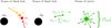 |
Fig. 1 Geometry of the collision event. In panel a two stars of mass M1 and M2 approach each other with velocities v1 and v2 in the frame of the black hole, respectively. In panel b the ejecta has mass Mej and consists of N equal-mass particles. The ejecta moves around the black hole with relative velocity vrel. In panel c we switch to the frame of the ejecta, in which each individual particle moves in a random direction with speed |vrel|. |
2 Method
We simulated the post-collision ejecta as N particles of equal mass arranged in a spherical distribution. For numerical ease, we considered ejecta with mass 1 M⊙, and note that for smaller or larger ejecta the mass accretion rate and therefore luminosity simply scale linearly with the mass of the ejecta. Benz & Hills (1987) conducted fully three-dimensional calculations of collisions between identical stars and found that in a grazing collision between two stars, at low enough speeds they are likely to form a spiral-shaped mass distribution which then proceeds to coalesce within a dynamical time. Mass loss then occurs through both direct ejection and formation of an accretion disk around the coalesced object.
We assumed that the ejecta with mass Mej continues moving around the SMBH with the same center-of-mass velocity as the two stars shortly before collision. This relative velocity is drawn from a Maxwellian distribution that describes a galaxy’s stellar density profile ρη(rgal) provided by Tremaine et al. (1994),
 (1)
(1)
where we adopted the commonly used value η = 2 (Hernquist 1990), Msph is the total mass of the host spheroid, and rs is a distinctive scaling radius. We note that the relative velocity can vary between 0 and a fraction of the speed of light because we were not including special and general relativistic corrections. Although mathematically the relative velocity is not constrained at the upper end, we note that in a typical calculation with tens of thousands of samples, the maximum relative velocity observed was no more than ~5% the speed of light.
An illustration of the configuration we considered is provided in Fig. 1. The left panel shows the geometry immediately prior to collision; two stars with masses M1, M2 and velocities v1, v2, with respect to the black hole, collide. Their relative velocity with respect to the black hole is vrel = v1 − v2. Conservation of momentum dictates that ejecta will continue moving with this same relative velocity after the collision for M1 = M2. For simplicity, we assumed this was the case. The middle panel shows the geometry immediately post-collision. We assumed our ejecta consists of N particles of equal mass which total Mej. The ejecta continues moving at vej with respect to the black hole. The right panel shows a close up of the ejecta from the middle panel, but now in the frame of the ejecta. Each of the N particles that make up the ejecta move in a random direction with speed |vrel|. Throughout our calculations, and as shown in Fig. 1, for the purposes of obtaining order-of-magnitude estimates, we did not consider the effects of dynamical friction from other stars in the vicinity.
In calculating this distribution it was assumed that the velocity vector has no preferred orientation. While this may be true, in our simulations the orientation of the velocity vector affected the overall form of the light curve. Therefore we must include the polar and azimuthal angles associated with the velocity vector as additional parameters. In the frame of the collision we also assumed that the N ejecta particles disperse in random directions, each with speed vrel. The end result is that from the frame of the viewer, for each of the N particles we added together two velocity vectors of the same magnitude but with two different, randomly generated directions-one which describes the overall velocity of the ejecta and another which describes the velocity of the individual particle. From the viewer’s perspective, particles travel at speeds ranging from 0 to 2vrel with an average value of vrel. In Fig. 2 we show an example where, with all other factors (mass of ejecta, mass of black hole, distance from black hole, magnitude of relative velocity vector) held constant, the angle of approach can have a significant effect on the overall shape of the light curve. In the corner of the plot, colored arrows indicate the relative velocity vector orientations with respect to the black hole, shown as a black dot at the center of the sphere.
We assumed that all particles start at the initial radius of the collision, rinit. From there, we must determine what path they take towards the black hole and how long they take to accrete in order to calculate the mass accretion radius. If we consider the ejecta particles to be freely moving test particles under Schwarzschild geometry, then they move along geodesics of spacetime. In the simplest case of radial infall, the proper time τ for a particle to move from some radius starting r to some final radius R is,
![Mathematical equation: $\tau = {\left( {{{{R^3}} \over {8{M_ \bullet }}}} \right)^{1/2}}\left[ {2{{\left( {{r \over R} - {{{r^2}} \over {{R^2}}}} \right)}^{1/2}} + {{\cos }^{ - 1}}\left( {{{2r} \over R} - 1} \right)} \right].$](/articles/aa/full_html/2024/10/aa50309-24/aa50309-24-eq2.png) (2)
(2)
We considered that some particles might initially move away from the black hole and then turn around. We assumed that each particle starts out with some energy  . If this theoretical turn-around radius exists, it should occur when the particle comes to a stop, rturn = −GM•/Einit.
In addition, we considered another important radius for the particle, the radius of closest approach. Given the particle’s initial angular momentum h = r × v this is described by,
 (3)
(3)
with e the eccentricity of the ejecta’s path around the black hole.
Finally, we considered how the time for the particle to fall inwards is affected by the accretion disk. As a particle moves within the accretion disk, it moves in a turbulent flow, losing both energy and angular momentum. We adopted the conventional alpha-disk model (Shakura & Sunyaev 1973) using the α parameter, α ≲ 1, which parametrizes the unknown effective increase in viscosity due to turbulent eddies within the accretion disk. In the alpha-disk model, we parametrize the kinematic velocity due to turbulence as v(R, t) = α a(R, t)H(R, t), with a(R, t) the sound speed and H(R, t) the disk thickness. Observations can be used to constrain α, which is typically calculated to vary between ~0.01 and ~0.1 (Lasota 2023). In our work, we adopted α = 0.1. At some radius R, we estimated the viscous accretion timescale as tacc = R2/v = R2/α a H. We estimated H ~ a/Ωk in an alpha disk, with Ωk = (r × v) /r2 the angular velocity. Finally, we estimated the sound speed as a ~ v/2, with v the Keplerian velocity, arriving at,
 (4)
(4)
with R the radius of closest approach and r and v the initial radius and velocity vectors of the particle. In our approach, we ignored the effect of gas pressure along the path of the debris towards the SMBH until the ejecta impacts the accretion disk. This is an approximate model that can be tested by hydrodynamic simulations in future work.
The final procedure for calculating the particle’s time to accrete was as follows: we first checked if the particle initially moves away from the SMBH before coming to a stop and turning around. If it did, we calculated the time this first segment takes assuming the particle moves along a geodesic of spacetime, i.e. that the effects of the accretion disk may be negligible in the immediate aftermath of the collision. Following this first step, all particles in the calculation were either at this turn-around radius or, if they did not turn around, then they were still at the radius of the collision. We then calculated the time it took for the particle to move to the radius of closest approach, again along a geodesic of spacetime. Finally, at the radius of closest approach, we calculated the corresponding viscous accretion timescale as given by the above equation. We added all the timescales together for each particle to arrive at its time to accrete.
Knowing each of the N particle’s mass and accretion timescale, we can translate this to a mass accretion rate. To translate the mass accretion rate to the luminosity, we needed the radiative efficiency. Because we are interested in comparing our final light curves to various TDEs with light curves in both the radio and optical regimes, we first estimated the fraction of energy we expect to be emitted in the radio frequency range. Cendes et al. (2022) studied TDE AT2018hyz flux density versus frequency measurements from VLA+ALMA, Chandra, UVOT, and ZTF data. This was integrated to find that approximately 5% of the energy was emitted in radio. For optical light curves, we adopted a value of 10% (Duras et al. 2020). We then considered the radiative efficiency of hot accretion flows. As described by Xie & Yuan (2012), we know that only a small fraction of the matter in the accretion disk will end up falling onto the black hole, and that electrons can receive a large fraction of the viscously dissipated energy in the accretion flow. Xie & Yuan (2012) provides a systematic calculation that takes in account both these considerations and provides fitting formulae of radiative efficiency as a function of accretion rate for various δ, the fraction of turbulent dissipation that heats the electrons directly,
 (5)
(5)
with  the accretion rate at the Schwarzschild radius,
  , and є0, a fitting constants provided in Table 1 of Xie & Yuan (2012).
Knowing each particle’s mass, time to accrete, the fraction of energy emitted in radio, and the radiative efficiency, we can calculate the luminosity associated with the fallback of the ejecta mass after the collision. However, we note that there is one more free parameter, which is the mass of the ejecta. At the start of calculations it was taken as 1 M⊙ for simplicity, but we note that the mass accretion rate scales linearly as the mass of the ejecta changes. While the luminosity would not necessarily scale linearly because the radiative efficiency is better described as multiple piecewise power-law equations that depend on the mass accretion rate, as long as the mass of the ejecta does not change by more than an order of magnitude, the change in the radiative efficiency rate is likely to have little effect, and we can generally guess that the new light curve can also be approximated by scaling the original light curve linearly with the change in the ejecta mass.
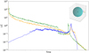 |
Fig. 2 Three different simulated collision events with the relative velocity vectors pointed in three different directions, as shown in the upper right hand corner of the plot. On the y-axis we plot the luminosity L divided by the average luminosity over the duration of the light curve |

3 TDE-like flares of interest
In this work we consider multiple potential TDEs studied in recent years, some of which have been noted for their unusual light curves. TDEs occur when the tidal force from the SMBH at some distance r from the SMBH for a star of mass M* and radius R*, GM•R*/r3, overwhelms the self-gravity of the star,  , which roughly occurs at some distance RT = (M•/M*)1/3R* known as the TDE radius (Hills 1975; Rees 1988). Furthermore, TDEs are expected to only be observable when the event happens outside of the SMBH’s Schwarzschild radius, which constrains observable events to occur around black holes with mass M• < 108 M⊙ for nonspinning black holes (Stone et al. 2019). The fallback timescale, defined as the orbital period of the most bound debris, follows tfb = 2πGM•(2E)−3/2, with E the energy of the most bound debris. If we further assume that the specific energy distribution is uniform, dE/dM = 0, we can derive that the fallback rate of TDE debris follows a power law, dM/dt ∝ (t − tD)−5/3 (Gezari 2021). Remarkably, this simply derived power law has been well-observed in optical light curves. Radio emission from a TDE was first detected during a multiwavelength campaign for the low-redshift optically selected TDE ASASSN-14li (Jose et al. 2014; van Velzen et al. 2016a). There are many interpretations of the radio emission, including synchrotron emission from external shocks (Alexander et al. 2016), the unbound debris stream (Krolik et al. 2016), a rela-tivistic jet (van Velzen et al. 2016b), and internal shocks in a relativistic jet (Pasham & van Velzen 2018). However, the detection of a correlation between the X-ray and radio light curves,
  (Pasham & van Velzen 2018) suggests that accretion and jet power are coupled, favoring the aforementioned internal jet model. Radio follow-up has shown that high radio-luminosity, relativistic jets occur in around ~1% of TDEs (Alexander et al. 2020).
It is difficult to do an exhaustive search of TDE light curves due to the varying ways they can be detected and the lack of a consolidated database. We chose to limit our focus to the last decade so we could study higher quality, more frequently sampled light curves. We searched the literature for transient events that have been classified as TDEs but noted to have nonstandard features, such as unusual late-time evolution or repeated flares. In the latter case, we excluded light curves with multiple repeated flares, which have been suggested to be partial tidal disruption events (Nixon et al. 2021). We also utilized systematic studies of large samples of TDEs, such as from Yao et al. (2023), in our search.
TDE AT2018hyz was first detected by the All-Sky Automated Survey for Supernovae (ASAS-SN, Shappee et al. 2014; Kochanek et al. 2017) on October 14,2018. The UV-Optical Telescope (UVOT, Roming et al. 2005) on board the Neil Gehrels Swift Observatory (Gehrels et al. 2004) subsequently observed AT2018hyz from November 10, 2018 until July 8, 2019. Four hours of AMI-LA observations on November 15, 2018, 32 days after optical discovery, revealed no radio source at the location of the transient. The upper limit of the observation corresponds to a luminosity of Lv < 6.6 × 1037 erg/s. The transient is located in the nucleus of the galaxy 2MASS J10065085+0141342 located at redshift z = 0.04573. Relative astrometry has been performed that the transient is nuclear, with a separation of 0.2 ± 0.8 kpc. AT2018hyz was then observed at 972 days with the Karl G. Jansky Very Large Array (VLA, Lacy et al. 2020) as part of a study of late-time radio emission from TDEs, which succeeded in detecting a source. Multi-frequency observations were then conducted from L- to K-band. This observed radio emission data, along with some collected by the VLA Low-band Ionosphere and Transient Experiment (VLITE), the MeerKAT radio telescope, and the Australian Telescope Compact Array (ATCA), is shown in the light curve in Fig. 3. As can be seen in the figure, the radio light curve shows the unusual feature of increasing rapidly from 7 × 1037 erg/s to 2 × 1039 erg/s over ~600 days. Gomez et al. (2020) uses the TDE package in the Python package MOSFiT to model the light curves and estimate a black hole mass of 5.2 × 10⁶ M⊙, which is in agreement with similar results found in Hung et al. (2020). In addition, the stellar velocity dispersion measured from the SDSS spectrum gives, using the M• − σ*. relation from (Xiao et al. 2011), can be used to estimate a black hole mass of 1.6 × 10⁶ M⊙. Given these various roughly consistent results, we adopt the last mass value in our work.
The second TDE-like flare we consider in this work is ASASSN-15oi. Observations of this transient from ASAS-SN first triggered the detection pipeline on August 14, 2015 (Brimacombe et al. 2015), from a location within the galaxy 2MASX J20390918-3045201. UVOT conducted follow-up observations in the UV and X-ray Telescope (XRT) (Burrows et al. 2005) confirmed its detection in the X-rays. Holoien et al. (2016) fits stellar population synthesis models to archival GALEX data, ASAS-SN V-band measurements, and 2MASS JHK_S magnitudes of the host galaxy to find a stellar mass of M* = 1.1 × 10¹⁰ M⊙, which implies a bulge mass of 6.3 × 10⁹ M⊙ based on the average stellar-mass-to-bulge-mass ratio from ASASSN-14ae and ASASSN-14li, which in turns implies a black hole mass of 1.3 × 10⁷ M⊙ using the Mbulge − M• relation (McConnell & Ma 2013). More recently, Gezari et al. (2017) and Mockler et al. (2019) arrived at a lower mass estimate of 2.5 × 10⁶ M⊙ using the aforementioned package MOSFiT. Immediately following optical discovery, VLA was used to carry out radio observations on ASASSN-15oi. Initial observations resulted in null detections. However, observations continued, motivated by theoretical models that suggest delayed signals may occur depending on how long the formation of the accretion disk takes. Null detections were recorded again at 23 and at 90 days. Significant radio emission was first detected at 182 days on February 12, 2016. Subsequently, a follow-up observation campaign was carried out in multiple radio frequencies, the results of which are displayed in figure AA. While the delayed radio flare at 182 days is surprising in itself, a second, even more surprising radio flare has since been detected years after the initial discovery in the optical. Various models have been considered to explain this unusual delayed emission, such as a standard CNM shockwave. model, a relativistic jet, and off-axis jet, and more. The existence of the second, even brighter flare makes all of these scenarios quite unlikely. It has been suggested that the rebrightening could be driven by whatever source caused the initially delayed radio emission, repeated partial disruptions of a star, or highly variable accretion due to the presence of a potential binary SMBH system. These proposed explanations still need to be tested against the available data.
In addition, we consider three UV and optical light curves composed of data gathered from ZTF (Bellm et al. 2019), the Asteroid Terrestrial-impact Last Alert System (ATLAS, Tonry et al. 2018), and UVOT on board the Neil Gehrels Swift Observatory (Gehrels et al. 2004). The events we consider are AT2019baf, AT2019ehz, and AT2021uqv, all three of which are chosen because in addition to their initial rises in luminosity, they also follow promising decay patterns similar to those seen in our simulations. For AT2019ehz, additional late radio emission is provided by Cendes et al. (2024). From Table 5 in Yao et al. (2023), we adopt black hole masses of log(M•/M⊙) = 6.89, 5.81, and 6.27, respectively, which are inferred either through M• − σ*. relations or through M• − Mgal relations if σ* measurements are not available. Their light curves, plotted as dark blue dots, are overlaid with our best-fit models, plotted as light blue curves, in Figs. 5–7
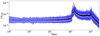 |
Fig. 3 Best-fitting simulated light curve to the AT2018hyz data is shown in black. Overlaid in blue are the ±1, 2σ confidence bands. |
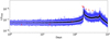 |
Fig. 4 Best-fitting simulated light curve to the ASASSN-15oi data is shown in black. Overlaid in blue are the ±1, 2σ confidence bands. |
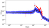 |
Fig. 5 Best-fitting simulated light curve to the AT2019baf data is shown in is shown in black. Overlaid in blue are the ±1, 2σ confidence bands. |
4 Analysis of results
We find that the accretion of the post-collision ejecta onto the black hole results in a light curve that can take on a varied appearance depending on several factors including the mass of the black hole, distance from the black hole at the time of collision, and direction of relative velocity vector. In this work, we focus on unusual observable traits we have noticed in our simulated light curves, which we believe can be used to distinguish these events from TDEs. For example, in some light curves we have observed a sudden, sharp initial rise in the luminosity. Other light curves can be distinguished by an initial decay in the luminosity followed by a rapid rise, another decay in the luminosity, one final smaller rise in the luminosity, and the final decay. In the latter case, the most distinctive feature of the complete light curve is the sustained rise in luminosity between the starting and ending periods of decaying luminosity. We refer to the duration of this sustained rise in luminosity as the “peak-to-peak timescale” tpp.
We are able to track the orbital parameters of particles as they accrete onto the black hole. Broadly speaking, we find that the first wave of particles accreting onto the black hole are those with orbits oriented directly towards the black hole. These are followed by particles on hyperbolic orbits (e > 1). Finally, particles that initially moved away from the black hole but eventually moved back towards the black hole are accreted.
Furthermore, we find that the duration of the increased luminosity period, tpp, scales with two other physical parameters of the system: 1) the distance the ejecta starts from the black hole divided by the Schwarzschild radius, rinit/rS, and 2) the mass of the SMBH, M•. When one of the two parameters is held constant and the other is allowed to vary, there exists a power law relation between tpp and the other parameter. We find that log(tpp) ∝ log(rinit/rs) and log(tpp) ∝ log(M•). These two relationships likewise follow the scaling relations that can be derived from the free-fall timecale as derived from Kepler’s third law,  , after substituting in the Schwarzschild radius for R to derive the correct relation with respect to M•. Examples of light curves with the this distinctive structure are shown in Fig. A.1. Along the x-axis, we vary rinit/rS. Along the y-axis, we vary M•. The angle of the relativity velocity vector is kept constant in all subplots. As can be seen in the figure, the duration of the flare, tpp, increases with both parameters. Given the overall reliance of tpp on M•, rinit/rS, and the direction of the relative velocity vector, knowing two of the three parameters (most likely the first two) could for determination of the third.
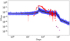 |
Fig. 6 Best-fitting simulated light curve to the AT2019ehz data is shown in is shown in black. Overlaid in blue are the ±1, 2σ confidence bands. In addition, late radio emissions are shown in purple. |
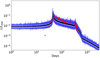 |
Fig. 7 Best-fitting simulated light curve to the AT2019ehz data is shown in is shown in black. Overlaid in blue are the ±1, 2σ confidence bands. |
5 Conclusions and future work
In this work we simulate light curves from stellar collision debris accreting onto a nearby SMBH, characterize the light curves, and compare them to observed TDE light curves. We consider TDEs in this work because, like the high-speed stellar collisions we are interested in, they occur at the centers of galaxies, making it possible for the two events to be confused and misidentified.
We identify that although the light curves may have a wide variety of appearances, some have the distinctive trait of a sudden sustained rise in luminosity, the duration of which can be predicted based on the mass of the SMBH and the distance from the black hole the ejecta started at. We show examples of how our simulated light curves can resemble observed data that has previously been classified as TDE events. In future work, we plan on more systematically fitting our model to TDE light curves from existing datasets to identify potential stellar collision candidates. In addition, recent TDE candidates displaying similar features in their optical light curves have been studied as Bowen fluorescence flares (Makrygianni et al. 2023; Koljonen et al. 2024). While a comparison between Bowen fluorescence flares and our proposed events lays beyond the scope of this paper, in future work the difference between the two should be studied in detail.
Although TDEs and stellar collisions can exist under similar circumstances, we highlight some important ways in which they can be distinguished. The stellar collision accretion flares described in this work are expected to be immediately preceded by a shorter, luminous flare as described in Hu & Loeb (2021). Partial tidal disruption events can result in repeated flares that can resemble the sustained flares in the light curves described in this work. However, partial tidal disruption events can also occasionally result in more than two flares from the continued disruption of the TDE debris (Bao et al. 2023; Miniutti et al. 2023). This long-term repeated behavior has not yet been demonstrated in stellar collision events.
Finally, TDEs are not expected to be observed in galaxies with SMBHs with M• ≳ 108M⊙ for nonspinning black holes (Stone et al. 2019), or M• ≳ 7 × 10⁸M⊙ for maximally spinning black holes (Kesden 2012), due to the TDE radius being too low. Stellar collisions can continue to occur in galaxies with SMBH masses this high, which means that an observation of the type described in this work in a galaxy with such a high-mass SMBH is unlikely to have originated from a TDE. Although higher mass SMBHs are less populous in our Universe (Behroozi et al. 2019), we will soon experience a substantial enhancement in survey power with the beginning of LSST.
Acknowledgements
We thank Hamsa Padmanabhan for providing constructive comments and discussion. B.X.H. and A.L. acknowledge support from the Black Hole Initiative, which is supported by the John Templeton Foundation and the Gordon and Betty Moore Foundation. B.X.H. acknowledges support from the Department of Defense National Defense Science and Engineering Graduate Fellowship.
Appendix A Additional Figure
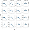 |
Fig. A.1 Example light curves from stellar collision debris accreting onto a BH. Along the horizontal axis, we vary the distance of the collision from the black hole, normalized by the Schwarzschild radius, rinit/rS. Along the vertical axis, we vary the mass of the supermassive black hole, M•. The y–axis of every plot is normalized by the Eddington luminosity for the black hole, LEdd. For all light curves shown here, the orientation is that shown by the yellow relative velocity vector in Fig. 2. |
References
- Alexander, K. D., Berger, E., Guillochon, J., Zauderer, B. A., & Williams, P. K. G. 2016, ApJ, 819, L25 [NASA ADS] [CrossRef] [Google Scholar]
- Alexander, K. D., van Velzen, S., Horesh, A., & Zauderer, B. A. 2020, Space Sci. Rev., 216, 81 [CrossRef] [Google Scholar]
- Balberg, S., Sari, R., & Loeb, A. 2013, MNRAS, 434, L26 [CrossRef] [Google Scholar]
- Bao, D.-W., Guo, W.-J., Zhang, Z.-X., et al. 2023, arXiv e-prints [arXiv:2311.16726] [Google Scholar]
- Behroozi, P., Wechsler, R. H., Hearin, A. P., & Conroy, C. 2019, MNRAS, 488, 3143 [NASA ADS] [CrossRef] [Google Scholar]
- Bellm, E. C., Kulkarni, S. R., Graham, M. J., et al. 2019, PASP, 131, 018002 [Google Scholar]
- Benz, W., & Hills, J. G. 1987, ApJ, 323, 614 [NASA ADS] [CrossRef] [Google Scholar]
- Brimacombe, J., Brown, J. S., Holoien, T. W. S., et al. 2015, ATel, 7910, 1 [Google Scholar]
- Burrows, D. N., Hill, J. E., Nousek, J. A., et al. 2005, Space Sci. Rev., 120, 165 [Google Scholar]
- Carter, B., & Luminet, J. P. 1982, Nature, 296, 211 [NASA ADS] [CrossRef] [Google Scholar]
- Carter, B., & Luminet, J. P. 1983, A&A, 121, 97 [Google Scholar]
- Cendes, Y., Berger, E., Alexander, K. D., et al. 2022, ApJ, 938, 28 [NASA ADS] [CrossRef] [Google Scholar]
- Cendes, Y., Berger, E., Alexander, K. D., et al. 2024, ApJ, 971, 185 [NASA ADS] [CrossRef] [Google Scholar]
- Donley, J. L., Brandt, W. N., Eracleous, M., & Boller, T. 2002, AJ, 124, 1308 [NASA ADS] [CrossRef] [Google Scholar]
- Duras, F., Bongiorno, A., Ricci, F., et al. 2020, A&A, 636, A73 [NASA ADS] [CrossRef] [EDP Sciences] [Google Scholar]
- Gehrels, N., Chincarini, G., Giommi, P., et al. 2004, ApJ, 611, 1005 [Google Scholar]
- Gezari, S. 2021, ARA&A, 59, 21 [NASA ADS] [CrossRef] [Google Scholar]
- Gezari, S., Cenko, S. B., & Arcavi, I. 2017, ApJ, 851, L47 [NASA ADS] [CrossRef] [Google Scholar]
- Gomez, S., Nicholl, M., Short, P., et al. 2020, MNRAS, 497, 1925 [NASA ADS] [CrossRef] [Google Scholar]
- Hernquist, L. 1990, ApJ, 356, 359 [Google Scholar]
- Hills, J. G. 1975, Nature, 254, 295 [Google Scholar]
- Holoien, T. W. S., Kochanek, C. S., Prieto, J. L., et al. 2016, MNRAS, 463, 3813 [NASA ADS] [CrossRef] [Google Scholar]
- Hu, B. X., & Loeb, A. 2024, A&A, 689, A23 [NASA ADS] [CrossRef] [EDP Sciences] [Google Scholar]
- Hung, T., Foley, R. J., Ramirez-Ruiz, E., et al. 2020, ApJ, 903, 31 [NASA ADS] [CrossRef] [Google Scholar]
- Ivezić, Ž., Kahn, S. M., Tyson, J. A., et al. 2019, ApJ, 873, 111 [Google Scholar]
- Jose, J., Guo, Z., Long, F., et al. 2014, ATel, 6777, 1 [Google Scholar]
- Kesden, M. 2012, Phys. Rev. D, 85, 024037 [NASA ADS] [CrossRef] [Google Scholar]
- Kochanek, C. S., Shappee, B. J., Stanek, K. Z., et al. 2017, PASP, 129, 104502 [Google Scholar]
- Koljonen, K. I. I., Liodakis, I., Lindfors, E., et al. 2024, MNRAS [arXiv:2403.04877] [Google Scholar]
- Krolik, J., Piran, T., Svirski, G., & Cheng, R. M. 2016, ApJ, 827, 127 [NASA ADS] [CrossRef] [Google Scholar]
- Lacy, M., Baum, S. A., Chandler, C. J., etal. 2020, PASP, 132, 035001 [Google Scholar]
- Lasota, J.-P. 2023, arXiv e-prints [arXiv:2302.07925] [Google Scholar]
- Lidskii, V. V., & Ozernoi, L. M. 1979, Sov. Astron. Lett., 5, 16 [NASA ADS] [Google Scholar]
- Makrygianni, L., Trakhtenbrot, B., Arcavi, I., et al. 2023, ApJ, 953, 32 [NASA ADS] [CrossRef] [Google Scholar]
- McConnell, N. J., & Ma, C.-P. 2013, ApJ, 764, 184 [Google Scholar]
- Miniutti, G., Giustini, M., Arcodia, R., et al. 2023, A&A, 670, A93 [NASA ADS] [CrossRef] [EDP Sciences] [Google Scholar]
- Mockler, B., Guillochon, J., & Ramirez-Ruiz, E. 2019, ApJ, 872, 151 [Google Scholar]
- Nixon, C. J., Coughlin, E. R., & Miles, P. R. 2021, ApJ, 922, 168 [NASA ADS] [CrossRef] [Google Scholar]
- Pasham, D. R., & van Velzen, S. 2018, ApJ, 856, 1 [Google Scholar]
- Predehl, P., Andritschke, R., Arefiev, V., et al. 2021, A&A, 647, A1 [EDP Sciences] [Google Scholar]
- Rees, M. J. 1988, Nature, 333, 523 [Google Scholar]
- Roming, P. W. A., Kennedy, T. E., Mason, K. O., et al. 2005, Space Sci. Rev., 120, 95 [Google Scholar]
- Rubin, D., & Loeb, A. 2011, Adv. Astron., 2011, 174105 [CrossRef] [Google Scholar]
- Shakura, N. I., & Sunyaev, R. A. 1973, A&A, 24, 337 [NASA ADS] [Google Scholar]
- Shappee, B., Prieto, J., Stanek, K. Z., et al. 2014, AAS Meeting Abstracts, 223, 236.03 [Google Scholar]
- Stone, N. C., Kesden, M., Cheng, R. M., & van Velzen, S. 2019, General Relativ. Grav., 51, 30 [Google Scholar]
- Tonry, J. L., Denneau, L., Heinze, A. N., et al. 2018, PASP, 130, 064505 [Google Scholar]
- Tremaine, S., Richstone, D. O., Byun, Y.-I., et al. 1994, AJ, 107, 634 [CrossRef] [Google Scholar]
- van Velzen, S., Anderson, G. E., Stone, N. C., et al. 2016a, Science, 351, 62 [NASA ADS] [CrossRef] [Google Scholar]
- van Velzen, S., Mendez, A. J., Krolik, J. H., & Gorjian, V. 2016b, ApJ, 829, 19 [NASA ADS] [CrossRef] [Google Scholar]
- Xiao, T., Barth, A. J., Greene, J. E., et al. 2011, ApJ, 739, 28 [NASA ADS] [CrossRef] [Google Scholar]
- Xie, F.-G., & Yuan, F. 2012, MNRAS, 427, 1580 [NASA ADS] [CrossRef] [Google Scholar]
- Yao, Y., Ravi, V., Gezari, S., et al. 2023, ApJ, 955, L6 [NASA ADS] [CrossRef] [Google Scholar]
- Yuan, W., Zhang, C., Chen, Y., & Ling, Z. 2022, in Handbook of X-ray and Gamma-ray Astrophysics (Berli: Springer), 86 [Google Scholar]
All Figures
|
Fig. 1 Geometry of the collision event. In panel a two stars of mass M1 and M2 approach each other with velocities v1 and v2 in the frame of the black hole, respectively. In panel b the ejecta has mass Mej and consists of N equal-mass particles. The ejecta moves around the black hole with relative velocity vrel. In panel c we switch to the frame of the ejecta, in which each individual particle moves in a random direction with speed |vrel|. |
| In the text | |
|
Fig. 2 Three different simulated collision events with the relative velocity vectors pointed in three different directions, as shown in the upper right hand corner of the plot. On the y-axis we plot the luminosity L divided by the average luminosity over the duration of the light curve |
| In the text | |
|
Fig. 3 Best-fitting simulated light curve to the AT2018hyz data is shown in black. Overlaid in blue are the ±1, 2σ confidence bands. |
| In the text | |
|
Fig. 4 Best-fitting simulated light curve to the ASASSN-15oi data is shown in black. Overlaid in blue are the ±1, 2σ confidence bands. |
| In the text | |
|
Fig. 5 Best-fitting simulated light curve to the AT2019baf data is shown in is shown in black. Overlaid in blue are the ±1, 2σ confidence bands. |
| In the text | |
|
Fig. 6 Best-fitting simulated light curve to the AT2019ehz data is shown in is shown in black. Overlaid in blue are the ±1, 2σ confidence bands. In addition, late radio emissions are shown in purple. |
| In the text | |
|
Fig. 7 Best-fitting simulated light curve to the AT2019ehz data is shown in is shown in black. Overlaid in blue are the ±1, 2σ confidence bands. |
| In the text | |
|
Fig. A.1 Example light curves from stellar collision debris accreting onto a BH. Along the horizontal axis, we vary the distance of the collision from the black hole, normalized by the Schwarzschild radius, rinit/rS. Along the vertical axis, we vary the mass of the supermassive black hole, M•. The y–axis of every plot is normalized by the Eddington luminosity for the black hole, LEdd. For all light curves shown here, the orientation is that shown by the yellow relative velocity vector in Fig. 2. |
| In the text | |
Current usage metrics show cumulative count of Article Views (full-text article views including HTML views, PDF and ePub downloads, according to the available data) and Abstracts Views on Vision4Press platform.
Data correspond to usage on the plateform after 2015. The current usage metrics is available 48-96 hours after online publication and is updated daily on week days.
Initial download of the metrics may take a while.