| Issue |
A&A
Volume 694, February 2025
|
|
|---|---|---|
| Article Number | A249 | |
| Number of page(s) | 12 | |
| Section | Planets, planetary systems, and small bodies | |
| DOI | https://doi.org/10.1051/0004-6361/202450142 | |
| Published online | 18 February 2025 | |
The role of cloud particle properties in the WASP-39b transmission spectrum based on JWST/NIRSpec observations
Escuela de Ingeniería de Bilbao, Universidad del País Vasco (UPV/EHU),
Bilbao,
Spain
★ Corresponding author; This email address is being protected from spambots. You need JavaScript enabled to view it.
; This email address is being protected from spambots. You need JavaScript enabled to view it.
Received:
27
March
2024
Accepted:
20
January
2025
Abstract
Context. Aerosols are capable of having a huge influence on reflected, emitted, and transmitted planetary spectra, especially at wavelengths similar to their average sizes, but also extending to much longer and shorter wavelengths. The Near InfraRed Spectrograph (NIRSpec) using the PRISM mode on board the James Webb Space Telescope (JWST) is providing valuable data of transit spectra over a wide spectral range that is able to cover the whole contribution of aerosols, potentially disentangling them from other constituents, and thus allowing us to constrain their properties.
Aims. Our aim was to investigate whether NIRSpec/PRISM JWST transmission spectroscopy observations, in addition to being useful for detecting and determining the abundance of gases more accurately than any previous instruments, are also capable of studying the physical properties of the aerosols in exoplanetary atmospheres.
Methods. We performed nested sampling Bayesian retrievals with the MultiNest library. We used the Planetary Spectrum Generator (PSG) and the Modelled Optical Properties of enSeMbles of Aerosol Particles (MOPSMAP) database as tools for the forward simulations and previously published NIRSpec/PRISM JWST observations of WASP-39b as input data.
Results. Retrievals indicate that models including an aerosol extinction weakly increasing or sharply decreasing with wavelength are decisively better than those with a flat transmission and that this increased degree of complexity is supported by the kind of data that JWST/NIRSpec can provide. Given other physical constraints from previous works, the scenario of weakly increasing particle extinction is favoured. We find that this also has an effect on the retrieved gas abundances.
Conclusions. JWST observations give us the potential to study some physical characteristics of exoplanetary clouds, in particular their overall dependence of transmissivity on wavelength. It is important to implement more detailed aerosol models as their extinction may affect significantly retrieved molecular abundances.
Key words: radiative transfer / methods: data analysis / techniques: spectroscopic / planets and satellites: atmospheres / planets and satellites: individual: WASP-39b
© The Authors 2025
 Open Access article, published by EDP Sciences, under the terms of the Creative Commons Attribution License (https://creativecommons.org/licenses/by/4.0), which permits unrestricted use, distribution, and reproduction in any medium, provided the original work is properly cited.
This article is published in open access under the Subscribe to Open model. This email address is being protected from spambots. You need JavaScript enabled to view it. to support open access publication.
1 Introduction
All the planets in the Solar System with a significant atmosphere have clouds and layers of aerosols (Sánchez-Lavega 2011). These ensembles of particles play an important role in the atmospheric energy budget by absorbing the incoming sunlight and blocking the outgoing thermal emission (de Pater & Lissauer 2015). Clouds are not only present in our closest neighbours; most of the hot Jupiters studied to date show clear evidence of having clouds in their atmospheres (Barstow et al. 2016; Sing et al. 2016; Tsiaras et al. 2018; Helling 2019; Barstow 2020).
Due to the viewing geometry, the transmission spectra obtained during primary transits are very sensitive to the presence of clouds in the exoatmospheres (Fortney 2005). Because of their opacity, clouds can block the stellar flux transmitted through the atmosphere and hide the spectral signals that would leave different molecules below them. Scattering effects caused by the aerosols can introduce slope-shaped effects in the observed spectra (Kreidberg 2018; Madhusudhan 2019).
The discovery of the planet WASP-39b was reported in 2011 by Faedi et al. (2011). It is a highly inflated Saturn-mass planet with a mass of 0.28 MJ and a radius of 1.27 RJ orbiting a G-type star. After its discovery, diverse studies considering different abundances of water, potassium, and sodium (Sing et al. 2016; Heng 2016; Fischer et al. 2016) tried to determine whether the planet had a cloudy atmosphere, but the results were not conclusive. Further works tended to show a favourable tendency towards the cloudy atmosphere (Barstow et al. 2016), but the idea of WASP-39b having a cloudy atmosphere was generally accepted when Wakeford et al. (2018) completed the planet spectrum with the near-infrared (NIR) spectral range using data from the Wide Field Camera 3 (WFC3) on board the Hubble Space Telescope (HST). Further analyses have continued treating WASP-39b as a cloudy planet, and have also tried to constrain the properties of the clouds (Tsiaras et al. 2018; Pinhas et al. 2018b; Fisher & Heng 2018; Pinhas et al. 2018a; Kirk et al. 2019).
Parametrising all the processes involved with clouds using the minimum number of parameters is a challenging task. Barstow (2020) presents a brief summary of the models used in the latest studies (Barstow et al. 2016; Tsiaras et al. 2018; Fisher & Heng 2018; Pinhas et al. 2018a). All these models are mainly focused on describing the vertical distribution of the cloud along the upper part of the atmosphere and determining at which pressure level it becomes opaque. They also tried to capture and to reproduce the wavelength dependence of the extinction efficiency of the cloud, but it is a difficult goal, due to the limited spectral range of the observations. Thus, most of the models treat cloud extinctions as flat or Rayleigh-shaped contributions.
This is where James Webb Space Telescope (JWST) starts playing a very important role in the study of clouds on exoplanets. Since its launch in December 2021, it has been observing transiting exoplanets with a much wider spectral range than any other previous instrument, such as those on board HST or the Spitzer Space Telescope. A wider range not only captures more gaseous absorption bands from potentially a greater number of species, but it is also better at constraining the smooth wavelength dependence of cloud opacity, as we investigate here.
For this work we used WASP-39b JWST observations already reduced and analysed in detail by previous works (Rustamkulov et al. 2023) in order to demonstrate the possible contribution of more sophisticated cloud particle models. A recent work by Lueber et al. (2024) has investigated the same data using the aerosol parametrisation proposed by Kitzmann & Heng (2017), but they were not able to disentangle aerosol properties from other contributions. Other works, such as Carone et al. (2023), have shown that the expected properties of the clouds and aerosols should be more complex than usually assumed. For this work, instead of computing aerosol distributions and properties from some ab initio hypotheses on the atmosphere, we investigated such characteristics by treating them as free parameters, as is commonly done in many studies of Solar System atmospheres. Our main goal is thus simply to try to determine an overall trend in the aerosol extinction, whether increasing, decreasing, or constant with wavelength assuming the minimal number of a priori hypotheses over their nature and properties.
To do so, we have structured this text as follows. In Sect. 2, we present the main characteristics of the observational data. In Sect. 3, we present the tools needed to perform the retrievals based on Bayesian inference and the model of the atmosphere that we have been using. In Sect. 4, we show the results obtained for the retrievals, and in Sect. 5 we summarise the conclusions that we have reached.
2 Data
The spectral data were taken from the supporting material of Rustamkulov et al. (2023). The observations were part of the JWST Transiting Exoplanet Community Early Release Science Program (ERS Program 1366). These data correspond to the 8.23-hour long transit of the planet WASP-39b from July 10, 2022, the first transit of the exoplanet observed with the Near InfraRed Spectrograph (NIRSpec) instrument of JWST using its PRISM mode. It covers the spectral range from 0.5 µm to 5.5 µm, visible to mid-infrared, with a resolving power of 20–300.
In Rustamkulov et al. (2023), four different data reductions are presented to extract the transmission spectra, although they demonstrated that all of these lead to equivalent overall results. However, to guide their discussions throughout the paper, they used the FIREFLy reduction (Rustamkulov et al. 2022). Thus, for an easier comparison, we have decided to also use the FIREFLy reduction as the observational input data.
Due to the brightness of WASP-39, the exoplanet observations are saturated in the region from 0.8 µm to 2.3 µm, but data reduction alleviated this effect and provided reasonable fluxes in that region. However, as the original work warns, the 0.9–1.5 micron range calibration remains questionable.
Prior to the JWST launch, there were only transmission spectra covering the wavelength range between 0.3 µm and 1.65 µm using the WFC3 and the Space Telescope Imaging Spectrograph (STIS) instruments of the HST. These observations were sometimes combined with wide photometric measurements from the Spitzer Space Telescope at 3.6 µm and 4.5 µm (Barstow et al. 2016; Changeat et al. 2022). However, the selected NIRSpec/PRISM covers a wavelength range from 0.5 to 5.5 µm, which, as we argue in the following sections, has unique capabilities for constraining aerosol properties. Figure 1 sketches the difference in the spectral ranges covered by these three different telescopes.
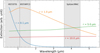 |
Fig. 1 Simulated transmissivity with MOPSMAP for spherical aerosols of different radii over the complete spectral range of JWST/NIRSpec- PRISM. The HST/STIS, HST/WFC3, and Spitzer/IRAC spectral ranges are delimited by grey backgrounds for comparison. |
3 Methodology
3.1 Tools
The forward simulations were executed using the Planetary Spectrum Generator (Villanueva et al. 2018) (hereafter PSG). It is a radiative transfer suite developed by NASA’s Goddard Space Flight Center team that allows the user to generate simulations of an extensive set of planetary bodies (both surfaces and atmospheres) over a wide spectral range. It is possible to simulate spectra for objects such as planets from the Solar System, exoplanets, or even comets. These simulated observations can be generated under the configuration of diverse instruments on board space telescopes, terrestrial observatories, or space missions. The user can modify a large variety of atmospheric and/or surface properties and parameters. It is also possible to define the geometry for the simulated observation (e.g. transiting exoplanets, nadir viewing or surface observations for landers).
Planetary spectra are generated using the core radiative- transfer model Planetary and Universal Model of Atmospheric Scattering (Villanueva et al. 2015; Smith et al. 2013), also known as PUMAS, which, using a one-dimensional and plane-parallel description of the atmosphere, computes high-resolution spectra via line-by-line calculations and moderate-resolution spectra using a correlated-k method. We used the line lists for H2O (Polyansky et al. 2018), CO2 (Yurchenko et al. 2020), CO (Li et al. 2015), SO2 (Gordon et al. 2022), Na (Allard et al. 2019), H2S (Gordon et al. 2022), CH4 (Yurchenko et al. 2024), and K (Allard et al. 2016). PUMAS takes into account the contribution of continuum processes such as Rayleigh scattering (Sneep & Ubachs 2005), refraction, UV broad absorption, and collision- induced absorption by H2 − H2 (Abel et al. 2011) and H2 – He (Abel et al. 2012). The radiative-transfer model also includes a multiple scattering modelling.
While the PSG online interface is very intuitive and didactic, it is also possible to install it locally through a Docker virtualisation system. Working locally with configuration files (with XML format) also allows speeding up the retrieval process by the use of the Application Program Interface (API) and the high-level programming language of the user’s choice.
PUMAS is able to include the contribution of aerosols, but the PSG suite only includes information for a limited set of them. However, it is possible to add custom aerosol information via the configuration file including the data about three different parameters. The extinction cross-section, Qext, is the attenuation coefficient normalised by the aerosol density and it characterises how effective the aerosol is in removing radiation from the incoming radiation beam. The single-scattering albedo, ϖ0, determines the ratio of scattered to extinguished (absorbed plus scattered) light from the incident beam. The asymmetry parameter, ɡ, represents the phase function (i.e. the directional distribution of the scattered light). Alternatively, aerosol phase functions can be provided in a much more detailed way using Legendre polynomials, but given the kind of data we are dealing with, this approach was not considered in this work. These quantities might be computed in different ways, using external databases such as Modelled Optical Properties of enSeMbles of Aerosol Particles (MOPSMAP) (see Sect. 3.2.3).
As commonly done for atmospheric retrievals, we employed a Bayesian approach (Madhusudhan et al. 2011; Benneke & Seager 2012; Lee et al. 2012; Line et al. 2013; Evans et al. 2016; Fisher & Heng 2018). We used MultiNest (Feroz et al. 2009; Buchner et al. 2014), an inference tool based on Nested Sampling Monte Carlo algorithms (Metropolis et al. 1953; Hastings 1970; Skilling 2006). Open-sources codes such as TauRex (Waldmann et al. 2015) or Helios-r2 (Kitzmann et al. 2020) already make use of MultiNest, but we developed our own code to engage it to PSG.
For each retrieval, MultiNest calculates the Bayesian evidence Z of the model under study. This value is related to the probability that the model is actually representing the real observations regardless of the value of its parameters. The comparison of the Bayesian evidence given by different models is the key to model selection. The Jeffrey’s scale (Jeffreys 1998; Trotta 2008), shown in Table 1, quantifies how much better one model is compared to another in terms of the Bayes factor. It is calculated as ln B1,2 = ln Z1 – ln Z2, where Z1 and Z2 are the Bayesian evidence values obtained for models 1 and 2, respectively. When the Bayes factor is bigger than 5.0, it is possible to state that one model is decisively better than the other. Nevertheless, when ln B1,2 is lower than 1 there is not enough evidence to claim which one is better. In this case Occam’s razor is followed: the model with the lowest number of free parameters is favoured.
MultiNest also returns the posterior probability distribution for each free parameter, thus allowing parameter determination. Following the law of large numbers, we assume the median of the marginalised probability distribution as the most likely value for each parameter. Similarly, uncertainties are calculated as 1σ deviations from that value. This is extremely important because in addition to getting a result, we can affirm whether our technique is sensitive enough to a parameter, and we are able to constrain a value with true physical meaning. In spite of the high dimensionality of the free parameter space, it is possible to visualise the correlation between parameters by plotting the marginalised probability distribution as a function of a pair of parameters, in what is often referred to as a corner plot.
Bayes factor values and their related evidence.
3.2 Atmospheric description
As stated before, PSG allows a huge number of options to define the atmosphere. In this subsection we show which atmospheric parameters are assumed as fixed in our models and which are left as free parameters. The size of the star, R∗, determines the total amount of light reaching the planet, while the planetary diameter, Dpl, constrains the planetary surface blocking the star light. We allowed these parameters to vary, but with the tight prior Gaussian distribution constraints calculated in Faedi et al. (2011): 179 000 ± 7000 km for Dpl and 0.895 ± 0.023 R⊙ for R∗.
The scale height represents how compressed or extended the atmosphere of a planet is. It depends on the planetary gravity, the atmospheric mean molecular weight and its temperature (Kreidberg 2018). We assume a Gaussian prior distribution for the planetary gravity of loɡ ɡ = 0.63 ± 0.05 (with ɡ in m s−2) based on Faedi et al. (2011). Both parameters, Dpl and loɡ ɡ, are referenced to the pressure reference level of 10 bar, which corresponds to the lowest layer of our model. The mean molecular weight is calculated based on the assumed molecular abundances.
3.2.1 Vertical profiles
In this section we discuss the vertical temperature and chemical species profiles. To describe them, we defined a log-uniform pressure profile with 40 levels between 10−6 and 101 bar.
As explained in Line et al. (2015), parametrising the temperature profile in planetary atmospheric retrievals is a challenging task. Different assumptions have been used for this purpose (see e.g. Guillot 2010; Line et al. 2015 or Kitzmann et al. 2020). We implemented the parametrisation of Kitzmann et al. (2020) to determine the temperature profile to be included in our study. This parametrisation is given in the log-pressure space and takes up to three free parameters: the bottom temperature and two vertical gradients for separate atmospheric levels. As we do not expect a thermal inversion in the atmsophere of WASP-39b (Baxter et al. 2020) we limited these slopes to be lower than 1.0. As a first step in our study, we performed three different retrievals, with one, two, and three free parameters, respectively, to describe the temperature profile. The isothermal profile is better than the two-parameter profile (ln B1,2 = 2.66) and much better than the three-parameter profile (ln B1,3 = 4.38) so we use this description for the rest of the paper.
We assumed an atmospheric temperature, Tiso, with a uniform prior distribution between 500 and 2000 K, although we expect to retrieve a value lower than the Teq = 1116 ± 32 K obtained by Faedi et al. (2011) since we are most likely sensitive to stratospheric levels, which are expected to have temperatures lower than the equilibrium temperature (Barstow et al. 2016).
The temperature profile is closely related to the molecular abundance profile of the atmosphere. We have defined the planet as mainly being composed of H2 and He, and at first instance we consider the presence of H2O, CO2 CO, SO2, and Na in the upper atmosphere, the chemical species with significant detections in Rustamkulov et al. (2023). Performing retrievals where the presence of other molecular abundances were individually included, we concluded that H2S (ln  ) must also be included in the simulations. Nevertheless CH4 (ln
  ) and K (ln BK = −0.60) did not show enough evidence to be taken into account. We consider a vertically uniform distribution for the molecular components. Fixing the abundance of hydrogen and helium, we let the volume mixing ratio of the rest of the abundances vary during retrievals with uniform prior distribution between 10−12 and 10−1.
3.2.2 Cloud vertical profiles
As mentioned in the introduction, the cloud vertical distribution along exoplanetary atmospheres plays an important role in the transit spectroscopy given that it can determine the height at which the atmosphere becomes opaque. As a first step in our study, we carried out a model selection to determine which cloud vertical profile best explains the observations. Once we had an indication of the best vertical cloud model, we were able to use it as a reference for the cloud extinction investigation.
We studied the most common vertical distributions in the literature. Model A has a uniform vertical distribution (Fisher & Heng 2018). Model B has a step-shaped opaque grey cloud distribution (Kreidberg et al. 2014). Model C has a step-shaped distribution (Benneke 2015; Barstow et al. 2016). Model D has a bottom opaque grey cloud combined with an upper uniform cloud (Tsiaras et al. 2018; Pinhas et al. 2018a). Model E has a slab parametrisation (Barstow et al. 2016). A graphic display of these vertical parametrisations can be found in Fig. 1 of Barstow (2020).
Models A and B are the simplest ones used in our simulations, each including only a single free parameter, respectively the aerosol abundance and the pressure-top level of the optically thick cloud. While it is not physically realistic to expect a uniform vertical distribution, this is justified by the fact that our simulations are only sensitive to a relatively narrow region of the atmosphere of around one or two decades in pressure.
A second degree of complexity is achieved with models C and D, which involve two free parameters. The step model C defines a uniform abundance for the lowest part of the atmosphere below a given pressure level and then no aerosols at all above that level. Model D defines the pressure-top level of the optically thick cloud and the aerosol abundance of the extended cloud above that same level.
Finally, model E defines a uniform distribution between two different pressure levels with no aerosol loading at the rest of the layers, thus requiring three free parameters.
3.2.3 Cloud extinction models
The effect of aerosols in our model is included using the three parameters presented in Sect. 3.1. Generally speaking, all of them depend on wavelength, which increases enormously the degeneracy of the problem. However, given the peculiar geometry for transmission spectroscopy, we find that ϖ0 and ɡ do not produce any significant variation in the simulations, in agreement with Barstow et al. (2016), and allow us to focus on Qext and its dependence on wavelength to compare cloud models.
Due to the relatively narrow wavelength range covered by observations prior to the JWST, most of the works on exoplanet atmospheres have assumed a flat or a Rayleigh-shaped (scattering efficiency scaling as 1/λ4) cloud transmissivity (Barstow et al. 2016). This can be understood from Fig. 1, which shows the simulated extinction over the entire spectral range of NIRSpec- PRISM for different spherical aerosol sizes. It can be seen how the transmissivity for each aerosol tends to peak at the wavelengths similar to their size, a conclusion that holds in general terms even for different particle shapes. Along HST spectral ranges, delimited by a grey background, small-sized aerosols match an extinction similar to a Rayleigh scattering and large-sized aerosols can be approximated with flat grey clouds. Nevertheless, this assumption cannot be extrapolated to the JWST spectral range where the 1/λ4 behaviour disappears for the small aerosols and where a flat transmissivity would underestimate the transmissivity at longer wavelengths.
We use as a reference the flat model (model I), where the value of Qext is constant with wavelength. As mentioned in the introduction, it is the simplest model that we could define and it is commonly used when studying the atmospheres of exoplanets. In order to compare with the flat cloud model, we defined a number of competing scenarios, each with a different dependence of Qext on wavelength.
Model II is the free slope model, in which we parametrise Qext as linearly dependent on wavelength leaving the slope, mCl, as a free parameter. Although there is no direct physical interpretation for this model, positive slope values would resemble larger particles, while negative slopes would mimic the behaviour of smaller particles. Thus, model II, including only one extra free parameter, is a simple first approach to modelling particle sizes.
Model III is based on the Ångström exponent. Ångström (1929) proposed that the optical thickness of an aerosol would behave with the wavelength of light as
 (1)
(1)
where α (always positive) is defined as the Ångström exponent. In this case, the parameter is inversely proportional to the particle size: the smaller the value of α, the bigger the aerosol. This cloud opacity dependence with wavelength has already been used in exoplanet atmospheric studies such as Lecavelier Des Etangs et al. (2008); MacDonald & Madhusudhan (2017); Pinhas et al. (2018a) or Barstow (2020).
Given that the optical thickness and the extinction crosssection are directly related, we can retrieve the best value for the Ångström parameter and build again the values of Qext(λ) using the value of reference by
 (2)
(2)
As it is possible that some aerosol distributions produce an opacity that grow with wavelength when covering the whole JWST spectral range (see Fig. 1), we decided to let the parameter α also reach negative values, which would result in opacity dependences similar to those produced by large aerosols. With this parametrisation we also included a steeper dependence with wavelength than the simple linear model discussed above.
A more realistic approach is achieved with cloud extinction model IV, which is generated using MOPSMAP (Gasteiger & Wiegner 2018), a database of optical properties of aerosol ensembles. The data set can provide the optical properties of single particles (or narrow size bins) on a grid of sizes, shapes, and refractive indices.
MOPSMAP allows the user to define the particles as spheres, spheroids, irregular bodies, or even a mixture of them. Aerosols present in exoplanet atmospheres must also have different shapes, but the latest literature shows that just determining particle sizes and composition is already a difficult issue (Kitzmann & Heng 2017). Thus, for simplicity, we defined the aerosols in our simulations with a spherical shape, as done for example in Ma et al. (2023) and Lueber et al. (2024). We note that such spherical shapes would leave a fingerprint in direct imaging observations at different phase angles and could potentially lead to the confirmation of spherical droplets the same way as was done for Venus (García Muñoz et al. 2014).
Whenever necessary, we used for the aerosols a log-normal size distribution (Hansen & Travis 1974), commonly used in Solar System atmospheric studies (Barstow et al. 2012; Anguiano-Arteaga et al. 2023; Toledo et al. 2019) and also used for brown dwarfs and exoplanets (Ackerman & Marley 2001; Benneke 2015). The amount of particles for a given size r is then described by
![Mathematical equation: $n(r) = {1 \over {\sqrt {2\pi } }}{1 \over {{\sigma _g}r}}\exp \left[ { - {1 \over 2}{{\left( {{{\ln r - \ln {r_g}} \over {{\sigma _g}}}} \right)}^2}} \right],$](/articles/aa/full_html/2025/02/aa50142-24/aa50142-24-eq5.png) (3)
(3)
where ln r𝑔 and σ𝑔 are respectively the mean and the standard deviation of the distribution in logarithmic scale. To describe this distribution, however, we used the effective radius, re f f, and the effective variance, υe f f, which are more intuitive when working with aerosol extinction since they are the mean and deviation of a size distribution weighted by the cross-section of the particles (Hansen & Travis 1974). They are related to the log-normal distribution parameters according to the following equations:
 (4)
(4)
 (5)
(5)
For the spectral properties of aerosols, MOPSMAP needs both the real and the imaginary part of the refractive index vector. This parameter is determined by the composition of the aerosols, with the real part describing the refraction of the particles and the imaginary part describing their absorption (Hansen & Travis 1974; Liou 1980).
We computed Qext(λ) data for different re f f particle distributions fixing rσ to 0.1. Given that we did not have any previous information about the composition or structure of the aerosols in WASP-39b, at the first instance we decided to fix both the real and the imaginary part of the refractive index at every wavelength to nr = 1.4 and ni = 0.0001. We discuss the potential role of the imaginary refractive index in the retrievals in Section 4.
There is an underlying assumption that must be taken with care: the Bayesian evidence for these different parametrisations are comparable to each other. Given that all of them only include one extra free parameter with respect to model I, and that the volumes of the parameter hyper-space are similar, we assume that it is possible to compare the evidence as in other cases. Table 2 summarises the prior probability distributions introduced in MultiNest for every free parameter included in the simulations.
4 Results and discussion
This section is organised as follows. We first discuss the results for determining the vertical cloud profile that most closely agrees with the observations. Then, using the best retrieved vertical profile, we perform the aerosol extinction model selection. Once we have a full description of the most plausible aerosol spectroscopic behaviour, we analyse how these assumptions affect the rest of free parameters of the retrievals. The idea is to bracket the retrievals with a range of possible assumptions to check the dependence of the obtained results with the description of the clouds and to determine their robustness. We lastly study the possibility of including molecular abundances initially discarded when using grey flat cloud extinctions, and study the sensitivity to other parameters, not initially considered, which may have an effect on the previous analyses.
Prior probability distributions for the free parameters included in the retrievals.
Logarithm of the Bayesian evidence obtained for the cloud vertical models and the relative Bayesian factor values when compared to the most likely model.
4.1 Vertical cloud profile model selection
Table 3 shows the Bayes factor obtained for each cloud vertical distribution model using the uniform model as reference, which is the simplest one. Based on Jeffrey’s scale (Table 1), all the cloud models seem quite similar in evidence with the exception of model B, the opaque step, which is clearly disfavoured by the data. Thus, given that model A gives the same evidence as the other models, but using the minimum number of free parameters, following Occam’s razor we conclude that the uniform vertical distribution is the best choice for describing the observations.
Inspecting retrieval results we realise that all vertical models have evolved towards a similar solution. We find that all vertical models, except model B, result in a distribution of particles that reaches τ = 1 in nadir geometry at levels between 100 mbar and 1 bar. At this level, the atmosphere has already become opaque and all the incoming stellar light is being blocked. Model B, instead, does not produce enough extinction at the upper levels, so it compensates for this lack of opacity placing the cloud top at higher atmospheric levels. As we have just stated, we henceforth proceed using the uniform cloud vertical profile.
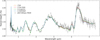 |
Fig. 2 Best fits for the cloud extinction models once their retrievals are finished. The observational data are shown as black and grey dots with error bars. |
Bayesian factor values obtained for the cloud extinction models when compared to the flat model.
4.2 Cloud extinction model selection
Table 4 shows the Bayes factor obtained for each cloud extinction model compared to the flat model and Fig. 2 shows the best fits to the observational data achieved in each retrieval. It is important to note that, even if all the different models reach a good fit with the observations, barely distinguishable between them, there is a clear difference in the retrieved evidence, meaning that the particle extinction model also plays a substantial role that can be constrained by the JWST observations.
Based on Table 1 we could argue that model III is the best choice for describing the aerosol opacity. As we can see in Fig. 3, which shows the retrieved aerosol opacities for each model, the Ångström model has evolved towards producing high optical depths at shorter wavelengths and a decrease towards longer wavelengths. For 1.0 µm it reaches values of τ = 1 at levels similar to the results for the flat extinction cloud, but at 4.0 µm, at the same pressure levels, it only reaches values of τ = 10−2−10−3. Nevertheless, in Fig. 3 we can observe a clear dichotomy. Models II and IV, not preferred in terms of Bayesian evidence, are not able to reach that heavy opacity decrease, generating instead opacities with a slight increase in wavelength in comparison to model I.
We thus suggest two possible aerosol opacity contributions when fitting Wasp-39b transit spectra. On the one hand, the opacity heavily decreases with wavelength, resembling the effect of small particles. As we show later, this aerosol model requires much higher molecular abundances to compensate for the thin cloud effect at longer wavelengths, and this also implies very high values for the mean molecular weight of the atmosphere of  . On the other hand, the slightly increase in opacity resembling the effect of big aerosol particles results in smaller molecular abundances with mean molecular weights more in line with those expected for the planet
  .
.
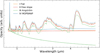 |
Fig. 3 Cloud opacity retrieved for each cloud extinction model in comparison to their total atmospheric opacity. |
4.3 Parametric study
Figures A.1 and A.2 show the corner plots obtained for model III and model IV, respectively, each of which is the most representative model of the cloud extinction behaviours already presented. The algorithm was sensitive enough to all the parameters, achieving Gaussian-like posterior distributions in all cases, perhaps with the exception of log H2S for model IV (see Fig. A.2). This means that the retrieval has always been capable of determining the most probable parameter value and its corresponding uncertainties. From the two figures we can see how, as previously claimed by Fisher & Heng (2018) and recently demonstrated in Lueber et al. (2024), the spectral resolution of JWST observations has enough potential to break the normalisation degeneracy. Retrievals performed with these observations show no correlation between the molecular abundances and the reference planetary diameter. Dpl shows only a strong correlation with the radius of the central star.
Model III shows a strong anticorrelation between the aerosol abundance and the parameter α. This is due to the strong requirement that the model should have a substantial particle extinction below 1 micron. In model IV, instead, there is a slight correlation between molecular and cloud abundances, as the thicker the cloud, the more gaseous absorption the model requires to fit the observed molecular bands. Lastly, it is possible to see in both corner plots the correlation between the retrieved volume mixing ratios of H2O and CO2, also noted in Lueber et al. (2024), due to their competing effects for shaping the peak around 2.8 µm.
The retrieved parameter values from the posterior distributions for models III and IV are summarised in Table 5. As expected, Dpl and R∗ are compatible with the prior distribution values included from Faedi et al. (2011). However, there is a discrepancy in the obtained value of lo𝑔 𝑔, which does not fit with the value given by Faedi et al. (2011) nor with that determined by Mancini et al. (2018). Obtaining the same discrepancy, Lueber et al. (2024) proposed that this enhanced value can be due to the retrieval trying to obtain a diminished scale height. As anticipated in Sect. 3, the retrieved Tiso value is somewhat lower than the Teq of Faedi et al. (2011).
For the retrieved chemical abundances, we make a comparison with recent works that have tried to constrain or at least detect different molecular abundances using different instrument observations. For the model III retrieval we obtained a value of log  with NIRSpec PRISM observations, compatible with the value ranging from −3 to −2.5 derived from the studies of Rustamkulov et al. (2023) employing the same instrument observations. Our water abundance calculation is also compatible with the values ranging from −3.3 to −1.4 derived from the Ahrer et al. (2023) studies with NIRCam observations; it is even consistent with the results (log H2O = −2.4 to −1.2) derived from Powell et al. (2024) using near-infrared JWST observations. Nevertheless, we obtained a slightly lower value than those derived from Fisher et al. (2024) and Feinstein et al. (2023) (log H2O = −2 to −1 and log H2O = −1.86, respectively), both employing Near Infrared Imager and Slitless Spectrograph (NIRISS) observations. A higher value of log H2O = −1.37 was also obtained by Wakeford et al. (2018) employing a combination of HST/WFC3, HST/STIS, Very Large Telescope (VLT), and Spitzer data. In addition, our H2O value is higher than those retrieved in Lueber et al. (2024) with the different JWST instrument observations, higher than the log H2O = −4.85 to −3.14 value retrieved with PRISM data in Constantinou et al. (2023), and higher than the value log
  derived from HST and Spitzer in Pinhas et al. (2018a). As explained in Fisher et al. (2024), these spread results expose the difficulty of measuring atmospheric chemical abundances, even with JWST observations.
From the strong footprints left by CO2 in the transit spectrum at 2.8 µm and 4.3 µm, we retrieved an abundance of log  . This value is higher than the value of log CO2 ≈ −5.0 retrieved from Ahrer et al. (2023) for atmospheric levels close to 1 bar, but is below the calculated value log
  using NIRISS observations in Fisher et al. (2024). For carbon monoxide we obtain a value of log
  higher than the values given by Grant et al. (2023) and Lueber et al. (2024) and the value derived from Extended Data Fig. 2 of Ahrer et al. (2023) (log CO = −2.63, log
  , and log CO ranging from −2 to −3, respectively).
For SO2, the expected chemical species producing the peak at 4 μm, we obtained a volume mixing ratio of log  . Rustamkulov et al. (2023) suggested values between –5 and –6 from NIRSpec PRISM observations, and Alderson et al. (2023) gave a value of log
  . And from near infrared JWST observations, Powell et al. (2024) proposed an abundance from −4.6 to −6.3. For sodium we obtained log
  compatible with the value of log
  obtained by Lueber et al. (2024) for its non-grey PRISM study, and for H2S we obtained log
  , an enhanced value when compared with the value obtained by Lueber et al. (2024) (H2S =
  ) and the derived value from Extended Data Fig. 2 of Ahrer et al. (2023) (H2S ≈ −3.5).
The results from model III are substantially higher than any other previous work, which makes sense, as none of them used such an extreme wavelength dependence with wavelength for the particle extinction. As already stated, such an enhanced molecular abundance would result in a huge molecular weight of  , which is probably unphysical.
However, the focus of this section is on the bias that the different cloud extinction models may have on the retrieved molecular abundances, especially when compared to the Flat Model. In Fig. 4, we show the retrieved molecular abundances for the four different cloud extinction models. The first thing that we can observe is how model III retrieved abundances are always higher, except for sodium, than those for the other models. As previously explained, it is due to the spectral shape of the retrieved cloud optical thickness. All the clouds reach similar τ values at shorter wavelengths, and thus similar Na opacities are required, but the model III cloud becomes optically thin at higher wavelengths, while the other clouds continue being opaque at those wavelengths. The lack of opacity is thus compensated by enhanced molecular abundances. While probably unrealistic, this is a clear warning that if our cloud extinction model is far from the real cloud, then our chemical abundances may be off by orders of magnitude.
The volume mixing ratios obtained for model IV are lower than those retrieved for model III, producing a mean molecular weight similar to the Jovian value. These results fit better with the previously stated bibliographic values for CO, SO2 , and H2S. In general, if clouds were composed of larger particles, using a flat cloud extinction model for the atmospheric retrievals could be a good approximation, but it could be overestimating some molecular abundances. For Wasp-39b we obtained with model II and model IV a cloud optical depth that increases slightly with wavelength, that could mask and compensate the effect that H2S would leave in the transmission spectrum, thus requiring a lower abundance.
As the different cloud extinction models are masking the required molecular opacities to fit the spectral observations, one could wonder if it could even compromise the detection of those chemical species. To find out, we repeated model III and model IV retrievals, but excluded the presence of CO, SO2, and H2S. The Bayes factors obtained for each gas removal retrieval when compared to the complete model retrieval are shown in Table 6. Model III always presents strong evidence to include all the chemical abundances. Nevertheless, model IV presents strong evidence to include CO and SO2, but not H2S. Following Occam’s Razor, the value In B = −0.86 is not enough to confirm the presence of that molecule in the atmosphere of the planet. We speculate that the slight increase in the cloud opacity with wavelength is masking the print that H2S would leave in the spectrum. It must be taken into account that these numbers consider the whole spectral range at the same time, not particular spectral windows, so this reasoning cannot substitute other detection processes that are much more sensitive.
Parameter a posteriori values and uncertainties.
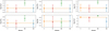 |
Fig. 4 Comparison of the retrieved chemical abundances for the different cloud extinction models: Flat model (I), Free slope model (II), Ångström model (III) and MOPSMAP model (IV). The horizontal line shows the value obtained for model I as a visual reference. |
Bayesian factor values obtained for cloud extinction models III and IV when excluding different chemical species in comparison to the original retrieval value.
4.4 Sensitivity to other parameters
Once the best cloud model was established, in the sense that it is the one with the strongest evidence supporting it, we tried to make further parametric sensitivity studies. We focus here on two main aspects. First, we included methane, as it has been shown to be an elusive component (Rustamkulov et al. 2023). The optically thin spectral behaviour of cloud extinction model III could possibly be partially compensated by extra molecular opacities, for example CH4. Second, we increased the complexity of our cloud particle descriptions, by means of adding or removing light absorption and checking if it affects the retrieved aerosol spectral behaviour. The first exploration implies adding the presence of CH4 to model III and model IV, as we describe in Sect. 3. For the second, we continued using in model IV a constant in wavelength imaginary refractive index, ni, but using its value as a new free parameter.
Regarding the inclusion of methane we obtained a Bayes factor In B1,2 = −0.52 when trying to incorporate it in model IV. This implies that the inclusion of CH4 to this model is not statistically supported. The upper limit retrieved for methane abundance is similar to those calculated in Rustamkulov et al. (2023); Ahrer et al. (2023), or Fisher et al. (2024), among others. Nevertheless, the calculated In B1,2 = 8.66 shows that there is evidence enough to include CH4 in our simulations when cloud extinction model III is implemented. In this case the algorithm retrieved a methane abundance of log  which also coincides with the upper limits of the works stated above.
On the other hand, the Bayes factor In B1,2 = −0.56 calculated when including ni as a free parameter to cloud extinction model IV shows that there is not enough evidence to be sensitive to the absorption of the aerosol. Posterior distributions for this retrieval show that any value of ni smaller than 10−2 is enough for reaching a good fit with the observations.
One final question would be whether or not an imaginary refractive index depending on wavelength would provide a good fit to the data. It should be noted that in most Solar System atmospheres the observed particles in the upper atmosphere are still to be identified and show unexpected absorptions (e.g. Toledo et al. 2019; Anguiano-Arteaga et al. 2023). As computation time makes this unfeasible for a complete exploration of the free parameter space, we show in Fig. 5 a preliminary exploration of this problem. We used upper and lower limits for the particle absorption for a number of particle sizes and tested how much the particle extinction may change. We find that very small particles show enormous differences depending on the actual values of the particle absorption, but particles with sizes around the observation wavelengths do not. This implies that composition, and hence ni(λ), would be of little relevance in transit geometry for the particle sizes obtained in this work, provided that they can be treated as Mie scatterers.
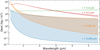 |
Fig. 5 Particle extinction as a function of wavelength for a few particle sizes (assumed spherical) and extreme values of imaginary refractive index ni = 10−2 and ni = 10−6 (solid coloured lines). The intermediate coloured areas represent all the possible values that extinction curve may take within the given limits. |
5 Conclusion
JWST observations have an enormous potential to start studying in depth the characteristics of clouds on exoplanets. The wider spectral range provided by instruments on board this telescope perfectly matches the smooth and extended extinction spectral footprint that can be expected from more realistic prescription of the aerosols. It has been demonstrated in this work how these more realistic prescriptions of the aerosols are strongly supported by the data and fit much better than other simpler models that have been usually assumed as a first educated guess for the problem.
In particular, we find that two different aerosol spectral behaviours are statistically favoured over a flat contribution: a heavy decreasing opacity with wavelength, resembling the effect of small particles, and a slight increase in opacity resembling the effect of larger aerosol particles. Nevertheless, after our last calculations, the increased retrieved mean molecular weight and the constraint of methane abundance despite the fact that it has not been detected in any previous works (e.g. Rustamkulov et al. 2023 or Lueber et al. 2024) has led us to consider that model III is not appropriate for defining the aerosol contribution when studying the atmosphere of Wasp-39b. Thus, we conclude that a cloud extinction model with an opacity slightly growing with wavelength is the most appropriate one. Specifically, Mie scattering from a particle distribution of effective radius around 3 µm is our best guess for fitting the observational data.
It has been shown that there is a significant difference between the retrieved atmospheric parameters obtained with more complex particle simulations and with the simpler flat model. It is important then to implement aerosol realistic simulations not only to get a better understanding of clouds on exoplanets, but also to avoid any bias in the rest of the parameters under study.
Nevertheless, we have also found some limitations to the degree of complexity that we can include in the aerosol spectral description. We found for example that there was not much sensitivity to the particle absorption, which would probably require a geometry different from the transit observations. Other particle properties, such as single-scattering albedos or scattering asymmetry factors, can be constrained using reflected light phase curves (Heng et al. 2021; Morris et al. 2024).
Acknowledgements
This work was supported by Grupos Gobierno Vasco IT1742-22. It has also been supported by grant PID2023-149055NB-C31 funded by MICIU/AEI/10.13039/501100011033 and FEDER, UE. J. Roy-Perez acknowledges a PhD scholarship from UPV/EHU. The authors acknowledge the effort of the scientists involved in JWST ERS programs and their contribution to the community. We thank Dr. G. Villanueva and the PSG team for the development of the tool and the support provided to the users.
Appendix A Additional figures
 |
Fig. A.1 Corner plot of the retrieval using the Ångström cloud extinction model (model III). The top plots for each column are the marginalised probability distribution for the different free parameters of the retrieval. The red lines are the fits of those distributions to a Gaussian function and the vertical dashed lines are the median and the 1 σ deviations. The rest of plots present the marginalised probability distributions as a function of a pair of parameters. The parameters are represented in the units shown in Table 5. Dpl , however, is represented in units of Jovian diameters. |
 |
Fig. A.2 Corner plot of the retrieval using the MOPSMAP cloud extinction model (model IV). The top plots for each column are the marginalised probability distributions for the different free parameters of the retrieval. The red lines are the fits of those distributions to a Gaussian function and the vertical dashed lines are the median and the 1 σ deviations. The rest of plots present the marginalised probability distributions as a function of a pair of parameters. The parameters are represented in the units shown in Table 5. Dpl, however, is represented in units of Jovian diameters. |
References
- Abel, M., Frommhold, L., Li, X., & Hunt, K. L. C. 2011, J. Phys. Chem. A., 115, 6805 [NASA ADS] [CrossRef] [Google Scholar]
- Abel, M., Frommhold, L., Li, X., & Hunt, K. L. C. 2012, J. Chem. Phys., 136, 044319 [NASA ADS] [CrossRef] [Google Scholar]
- Ackerman, A. S., & Marley, M. S. 2001, ApJ, 556, 872 [Google Scholar]
- Ahrer, E.-M., Alderson, L., Batalha, N. M., et al. 2023, Nature, 614, 649 [NASA ADS] [CrossRef] [Google Scholar]
- Alderson, L., Wakeford, H. R., Alam, M. K., et al. 2023, Nature, 614, 664 [NASA ADS] [CrossRef] [Google Scholar]
- Allard, N. F., Spiegelman, F., & Kielkopf, J. F. 2016, A&A, 589, A21 [NASA ADS] [CrossRef] [EDP Sciences] [Google Scholar]
- Allard, N. F., Spiegelman, F., Leininger, T., & Molliere, P. 2019, A&A, 628, A120 [NASA ADS] [CrossRef] [EDP Sciences] [Google Scholar]
- Anguiano-Arteaga, A., Pérez-Hoyos, S., Sánchez-Lavega, A., Sanz-Requena, J. F., & Irwin, P. G. J. 2023, JGR Planets, 128, e2022JE007427 [CrossRef] [Google Scholar]
- Ångström, A. 1929, Geografis. Ann., 11, 156 [Google Scholar]
- Barstow, J. K. 2020, MNRAS, 497, 4183 [Google Scholar]
- Barstow, J., Tsang, C., Wilson, C., et al. 2012, Icarus, 217, 542 [NASA ADS] [CrossRef] [Google Scholar]
- Barstow, J. K., Aigrain, S., Irwin, P. G. J., & Sing, D. K. 2016, ApJ, 834, 50 [NASA ADS] [CrossRef] [Google Scholar]
- Baxter, C., Désert, J.-M., Parmentier, V., et al. 2020, A&A, 639, A36 [EDP Sciences] [Google Scholar]
- Benneke, B. 2015, arXiv e-prints [arXiv:1504.07655] [Google Scholar]
- Benneke, B., & Seager, S. 2012, ApJ, 753, 100 [NASA ADS] [CrossRef] [Google Scholar]
- Buchner, J., Georgakakis, A., Nandra, K., et al. 2014, A&A, 564, A125 [NASA ADS] [CrossRef] [EDP Sciences] [Google Scholar]
- Carone, L., Lewis, D. A., Samra, D., Schneider, A. D., & Helling, C. 2023, arXiv e-prints [arXiv:2301.08492] [Google Scholar]
- Changeat, Q., Edwards, B., Al-Refaie, A. F., et al. 2022, ApJS, 260, 3 [NASA ADS] [CrossRef] [Google Scholar]
- Constantinou, S., Madhusudhan, N., & Gandhi, S. 2023, ApJ, 943, L10 [NASA ADS] [CrossRef] [Google Scholar]
- de Pater, I., & Lissauer, J. J. 2015, Planetary Sciences, 2nd edn. (Cambridge University Press) [Google Scholar]
- Evans, T. M., Sing, D. K., Wakeford, H. R., et al. 2016, ApJ, 822, L4 [NASA ADS] [CrossRef] [Google Scholar]
- Faedi, F., Barros, S. C. C., Anderson, D. R., et al. 2011, A&A, 531, A40 [NASA ADS] [CrossRef] [EDP Sciences] [Google Scholar]
- Feinstein, A. D., Radica, M., Welbanks, L., et al. 2023, Nature, 614, 670 [NASA ADS] [CrossRef] [Google Scholar]
- Feroz, F., Hobson, M. P., & Bridges, M. 2009, MNRAS, 398, 1601 [NASA ADS] [CrossRef] [Google Scholar]
- Fisher, C., & Heng, K. 2018, MNRAS, 481, 4698 [Google Scholar]
- Fischer, P. D., Knutson, H. A., Sing, D. K., et al. 2016, ApJ, 827, 19 [CrossRef] [Google Scholar]
- Fisher, C., Taylor, J., Parmentier, V., et al. 2024, MNRAS, 535, 27 [NASA ADS] [CrossRef] [Google Scholar]
- Fortney, J. J. 2005, MNRAS, 364, 649 [Google Scholar]
- García Muñoz, A., Pérez-Hoyos, S., & Sánchez-Lavega, A. 2014, A&A, 566, L1 [NASA ADS] [CrossRef] [EDP Sciences] [Google Scholar]
- Gasteiger, J., & Wiegner, M. 2018, GMD, 11, 2739 [NASA ADS] [Google Scholar]
- Gordon, I., Rothman, L., Hargreaves, R., et al. 2022, J. Quant. Spec. Radiat. Transf., 277, 107949 [NASA ADS] [CrossRef] [Google Scholar]
- Grant, D., Lothringer, J. D., Wakeford, H. R., et al. 2023, ApJ, 949, L15 [NASA ADS] [CrossRef] [Google Scholar]
- Guillot, T. 2010, A&A, 520, A27 [NASA ADS] [CrossRef] [EDP Sciences] [Google Scholar]
- Hansen, J. E., & Travis, L. D. 1974, Space Sci. Rev., 16, 527 [Google Scholar]
- Hastings, W. K. 1970, Biometrika, 57, 97 [Google Scholar]
- Helling, C. 2019, Annu. Rev. Earth Planet. Sci., 47, 583 [CrossRef] [Google Scholar]
- Heng, K. 2016, ApJ, 826, L16 [NASA ADS] [CrossRef] [Google Scholar]
- Heng, K., Morris, B. M., & Kitzmann, D. 2021, Nat. Astron., 5, 1001 [NASA ADS] [CrossRef] [Google Scholar]
- Jeffreys, H. 1998, The Theory of Probability (OuP Oxford) [Google Scholar]
- Kirk, J., López-Morales, M., Wheatley, P. J., et al. 2019, ApJ, 158, 144 [Google Scholar]
- Kitzmann, D., & Heng, K. 2017, MNRAS, 475, 94 [Google Scholar]
- Kitzmann, D., Heng, K., Oreshenko, M., et al. 2020, ApJ, 890, 174 [Google Scholar]
- Kreidberg, L. 2018, Exoplanet Atmosphere Measurements from Transmission Spectroscopy and Other Planet Star Combined Light Observations, eds. H. J. Deeg, & J. A. Belmonte (Cham: Springer International Publishing), 2083 [Google Scholar]
- Kreidberg, L., Bean, J. L., Désert, J.-M., et al. 2014, Nature, 505, 69 [Google Scholar]
- Lecavelier Des Etangs, A., Pont, F., Vidal-Madjar, A., & Sing, D. 2008, A&A, 481, L83 [NASA ADS] [CrossRef] [Google Scholar]
- Lee, J. M., Fletcher, L. N., & Irwin, P. G. J. 2012, MNRAS, 420, 170 [NASA ADS] [CrossRef] [Google Scholar]
- Li, G., Gordon, I. E., Rothman, L. S., et al. 2015, ApJS, 216, 15 [NASA ADS] [CrossRef] [Google Scholar]
- Line, M. R., Wolf, A. S., Zhang, X., et al. 2013, ApJ, 775, 137 [NASA ADS] [CrossRef] [Google Scholar]
- Line, M. R., Teske, J., Burningham, B., Fortney, J. J., & Marley, M. S. 2015, ApJ, 807, 183 [NASA ADS] [CrossRef] [Google Scholar]
- Liou, K. N. 1980, An Introduction to Atmospheric Radiation (New York: Academic Press) [Google Scholar]
- Lueber, A., Novais, A., Fisher, C., & Heng, K. 2024, A&A, 687, A110 [NASA ADS] [CrossRef] [EDP Sciences] [Google Scholar]
- Ma, S., Ito, Y., Al-Refaie, A. F., et al. 2023, ApJ, 957, 104 [NASA ADS] [CrossRef] [Google Scholar]
- MacDonald, R. J., & Madhusudhan, N. 2017, MNRAS, 469, 1979 [Google Scholar]
- Madhusudhan, N. 2019, ARA&A, 57, 617 [NASA ADS] [CrossRef] [Google Scholar]
- Madhusudhan, N., Harrington, J., Stevenson, K. B., et al. 2011, Nature, 469, 64 [NASA ADS] [CrossRef] [Google Scholar]
- Mancini, L., Esposito, M., Covino, E., et al. 2018, A&A, 613, A41 [NASA ADS] [CrossRef] [EDP Sciences] [Google Scholar]
- Metropolis, N., Rosenbluth, A. W., Rosenbluth, M. N., Teller, A. H., & Teller, E. 1953, J. Chem. Phys., 21, 1087 [Google Scholar]
- Morris, B. M., Heng, K., & Kitzmann, D. 2024, A&A, 685, A104 [NASA ADS] [CrossRef] [EDP Sciences] [Google Scholar]
- Pinhas, A., Madhusudhan, N., Gandhi, S., & MacDonald, R. 2018a, MNRAS, 482, 1485 [Google Scholar]
- Pinhas, A., Rackham, B. V., Madhusudhan, N., & Apai, D. 2018b, MNRAS, 480, 5314–5331 [NASA ADS] [CrossRef] [Google Scholar]
- Polyansky, O. L., Kyuberis, A. A., Zobov, N. F., et al. 2018, MNRAS, 480, 2597 [NASA ADS] [CrossRef] [Google Scholar]
- Powell, D., Feinstein, A. D., Lee, E. K. H., et al. 2024, Nature, 626, 979 [NASA ADS] [CrossRef] [Google Scholar]
- Rustamkulov, Z., Sing, D. K., Liu, R., & Wang, A. 2022, ApJ, 928, L7 [CrossRef] [Google Scholar]
- Rustamkulov, Z., Sing, D. K., Mukherjee, S., et al. 2023, Nature, 614, 659 [NASA ADS] [CrossRef] [Google Scholar]
- Sánchez-Lavega, A. 2011, An Introduction to Planetary Atmospheres (Florida, USA: Taylor & Francis Group) [Google Scholar]
- Sing, D. K., Fortney, J. J., Nikolov, N., et al. 2016, Nature, 529, 59 [Google Scholar]
- Skilling, J. 2006, Bayesian Anal., 1, 833 [Google Scholar]
- Smith, M. D., Wolff, M. J., Clancy, R. T., Kleinböhl, A., & Murchie, S. L. 2013, JGR Planets, 118, 321 [CrossRef] [Google Scholar]
- Sneep, M., & Ubachs, W. 2005, J. Quant. Spec. Radiat. Transf., 92, 293 [NASA ADS] [CrossRef] [Google Scholar]
- Toledo, D., Irwin, P. G. J., Rannou, P., et al. 2019, Icarus, 333, 1 [NASA ADS] [CrossRef] [Google Scholar]
- Trotta, R. 2008, Contemp. Phys., 49, 71 [Google Scholar]
- Tsiaras, A., Waldmann, I. P., Zingales, T., et al. 2018, AJ, 155, 156 [NASA ADS] [CrossRef] [Google Scholar]
- Villanueva, G. L., Mumma, M. J., Novak, R. E., et al. 2015, Science, 348, 218 [Google Scholar]
- Villanueva, G. L., Smith, M. D., Protopapa, S., Faggi, S., & Mandell, A. M. 2018, J. Quant. Spec. Radiat. Transf., 217, 86 [NASA ADS] [CrossRef] [Google Scholar]
- Wakeford, H. R., Sing, D. K., Deming, D., et al. 2018, AJ, 155, 29 [Google Scholar]
- Waldmann, I. P., Tinetti, G., Rocchetto, M., et al. 2015, ApJ, 802, 107 [CrossRef] [Google Scholar]
- Yurchenko, S. N., Mellor, T. M., Freedman, R. S., & Tennyson, J. 2020, MNRAS, 496, 5282 [NASA ADS] [CrossRef] [Google Scholar]
- Yurchenko, S. N., Owens, A., Kefala, K., & Tennyson, J. 2024, MNRAS, 528, 3719 [CrossRef] [Google Scholar]
All Tables
Prior probability distributions for the free parameters included in the retrievals.
Logarithm of the Bayesian evidence obtained for the cloud vertical models and the relative Bayesian factor values when compared to the most likely model.
Bayesian factor values obtained for the cloud extinction models when compared to the flat model.
Bayesian factor values obtained for cloud extinction models III and IV when excluding different chemical species in comparison to the original retrieval value.
All Figures
|
Fig. 1 Simulated transmissivity with MOPSMAP for spherical aerosols of different radii over the complete spectral range of JWST/NIRSpec- PRISM. The HST/STIS, HST/WFC3, and Spitzer/IRAC spectral ranges are delimited by grey backgrounds for comparison. |
| In the text | |
|
Fig. 2 Best fits for the cloud extinction models once their retrievals are finished. The observational data are shown as black and grey dots with error bars. |
| In the text | |
|
Fig. 3 Cloud opacity retrieved for each cloud extinction model in comparison to their total atmospheric opacity. |
| In the text | |
|
Fig. 4 Comparison of the retrieved chemical abundances for the different cloud extinction models: Flat model (I), Free slope model (II), Ångström model (III) and MOPSMAP model (IV). The horizontal line shows the value obtained for model I as a visual reference. |
| In the text | |
|
Fig. 5 Particle extinction as a function of wavelength for a few particle sizes (assumed spherical) and extreme values of imaginary refractive index ni = 10−2 and ni = 10−6 (solid coloured lines). The intermediate coloured areas represent all the possible values that extinction curve may take within the given limits. |
| In the text | |
|
Fig. A.1 Corner plot of the retrieval using the Ångström cloud extinction model (model III). The top plots for each column are the marginalised probability distribution for the different free parameters of the retrieval. The red lines are the fits of those distributions to a Gaussian function and the vertical dashed lines are the median and the 1 σ deviations. The rest of plots present the marginalised probability distributions as a function of a pair of parameters. The parameters are represented in the units shown in Table 5. Dpl , however, is represented in units of Jovian diameters. |
| In the text | |
|
Fig. A.2 Corner plot of the retrieval using the MOPSMAP cloud extinction model (model IV). The top plots for each column are the marginalised probability distributions for the different free parameters of the retrieval. The red lines are the fits of those distributions to a Gaussian function and the vertical dashed lines are the median and the 1 σ deviations. The rest of plots present the marginalised probability distributions as a function of a pair of parameters. The parameters are represented in the units shown in Table 5. Dpl, however, is represented in units of Jovian diameters. |
| In the text | |
Current usage metrics show cumulative count of Article Views (full-text article views including HTML views, PDF and ePub downloads, according to the available data) and Abstracts Views on Vision4Press platform.
Data correspond to usage on the plateform after 2015. The current usage metrics is available 48-96 hours after online publication and is updated daily on week days.
Initial download of the metrics may take a while.