| Issue |
A&A
Volume 690, October 2024
|
|
|---|---|---|
| Article Number | A51 | |
| Number of page(s) | 24 | |
| Section | Astrophysical processes | |
| DOI | https://doi.org/10.1051/0004-6361/202449953 | |
| Published online | 01 October 2024 | |
Bayesian sensitivity of binary pulsars to ultra-light dark matter
1
CEICO, FZU–Institute of Physics of the Czech Academy of Sciences, Na Slovance 2, 182 00 Praha 8, Czech Republic
2
Charles University, Faculty of Mathematics and Physics, Institute of Theoretical Physics, V Holešovičkách 2, 180 00 Praha 8, Czech Republic
3
Universidad de Buenos Aires, Facultad de Ciencias Exactas y Naturales, Departamento de Física, Buenos Aires, Argentina
4
CONICET – Universidad de Buenos Aires, Instituto de Física de Buenos Aires (IFIBA), Buenos Aires, Argentina
Received:
12
March
2024
Accepted:
5
June
2024
Ultra-light dark matter perturbs the orbital motion of binary pulsars, in particular by causing peculiar time variations of a binary’s orbital parameters, which then induce variations in the pulses’ times of arrival. Binary pulsars have therefore been shown to be promising detectors of ultra-light dark matter. To date, the sensitivity of binary pulsars to ultra-light dark matter has only been studied for dark matter masses in a narrow resonance band around a multiple of the binary pulsar orbital frequency. In this study we devise a two-step, bayesian method that enables us to compute semi-analytically the sensitivity for all masses, also away from the resonance, and to combine several observed binaries into one global sensitivity curve. We then apply our method to the case of a universal, linearly-coupled, scalar ultra-light dark matter. We find that with next-generation radio observatories the sensitivity to the ultra-light dark matter coupling will surpass that of Solar-System constraints for a decade in mass around m ∼ 10−21 eV, even beyond resonance
Key words: binaries: general / pulsars: general / dark matter
© The Authors 2024
 Open Access article, published by EDP Sciences, under the terms of the Creative Commons Attribution License (https://creativecommons.org/licenses/by/4.0), which permits unrestricted use, distribution, and reproduction in any medium, provided the original work is properly cited.
This article is published in open access under the Subscribe to Open model. Subscribe to A&A to support open access publication.
1. Introduction
Binary pulsars, namely astrophysical binary systems in which at least one of the two orbiting bodies is a pulsar, are outstandingly precise clocks, and as such they have been used in a wide variety of applications–readers can refer to Lorimer (2008) for a comprehensive review. Among those applications, binary pulsars can act as potential detectors for dark matter whose mass lies in the lower end of the ultra-light dark matter (ULDM) range: 10−23 eV ≲ m ≲ 10−18 eV. In the late Universe, ULDM with such a mass behaves like a coherent superposition of oscillators all with the same inverse frequency of about 1.15 hours × (10−18 eV/m), which roughly corresponds to the span of periods of observed binary pulsars. Two interesting phenomena take place when the orbital period of the system, or any of its harmonics, is in resonance with the ULDM oscillations. First, because the ULDM oscillations perturb the gravitational potential in which the binary system is immersed, they cause secular drifts in the orbital motion, which however are unlikely to be observed. Second, if the ULDM carries a (fifth) force that couples directly to the bodies of the binary system, it brings about further secular drifts in the orbital parameters that can be potentially detected1. Such resonant effects have been studied for ULDM of spin 0, spin 1 and spin 2 Blas et al. (2017, 2020), López Nacir & Urban (2018), Armaleo et al. (2020a), and in all cases binary pulsars have been shown to be promising detectors for such kinds of ULDM
These results however are limiting in three respects. First, resonances appear only for a very narrow range of ULDM mass m peaked at a given harmonic of the orbital period; for the linear direct coupling we consider here m ≈ kωb where  is the harmonic number and ωb = 2π/Pb is the orbital frequency and Pb the orbital period. This means that each binary system can probe a very small parameter space in ULDM mass, or, in other words, that only very few, if any, binary pulsars are sensitive to ULDM. Second, for the most-studied case of a universally-coupled spin 0, the resonant secular drift on the period Pb–which is often the best-measured parameter–vanishes for systems with small eccentricities e → 0, which are the majority (e.g. more than 80% in the ATNF catalogue Manchester et al. (2005) have e < 0.001)2. Hence, in this case we are limited to an even smaller sub-sample of all observed binary pulsars. Third, so far the sensitivity of binary pulsars to ULDM has only been estimated by requiring that the ULDM effects be within the errors of the measured orbital parameters, thus ignoring the time behaviour of the ULDM perturbations on the orbital parameters
In this work we develop a new method to estimate the sensitivity of binary pulsars as detectors of ULDM. For practical purposes here we limit ourselves to the universally-coupled linear scalar case, but our results are readily generalised to other spins and types of coupling. Our proposal draws from existing methods used to determine the sensitivity of pulsar-timing arrays to continuous gravitational waves, and takes advantage of the full time evolution of the ULDM perturbations to the binary system. In this way we are able to improve on existing results in three different ways. First, for a given system, we are able to compute semi-analytically the sensitivity to ULDM for all values of the ULDM mass, that is, also away from the resonance. Second, since we are not limited to resonances, the effects of ULDM do not vanish for e → 0, only the resonances do; hence, even for a universally-coupled scalar ULDM, all binary pulsars can act as ULDM detectors. Third, with our method we can straightforwardly combine multiple binary pulsars, each of which spans the entire mass range of interest. This vastly improves the sensitivity to ULDM and can tighten the constraint on the ULDM parameter space should no signal be found
The rest of this paper is organised as follows: in Sect. 2 we introduce the post-Keplerian, osculating-orbits formalism and derive the effects of ULDM on the six orbital parameters. In Sect. 3 we describe our method to estimate the sensitivity. We present our results in Sect. 4 and conclude with an outlook for future work in Sect. 5. In the Appendix we collect several useful formulas and additional tests and cross-checks of our method. Throughout the paper we use units for which c = 1 and ℏ = 1
2. The perturbed orbital motion
2.1. Timing models
The phase N of the pulsar at the moment at which the pulse is emitted is related to the proper time as measured by a hypothetical clock on the pulsar T by
where ν is the spin frequency of the pulsar and N0 an arbitrary constant–readers can refer to Lorimer & Kramer (2004). The pulsar’s proper time T is related to the time of arrival of each pulse at the detector on Earth through a timing model. In this work we focus on two timing models, the BT model of Blandford & Teukolsky (1976) and the ELL1 model of Lange et al. (2001), which better describes near-circular orbits
For non-relativistic orbits the relation between proper and Earth’s times can be written as

where we defined

where a is the semi-major axis of the binary, e its eccentricity, ι its inclination, ω the argument of periapsis (not to be confused with the orbital frequency ωb), and M1 and M2 are the masses of the pulsars and its companion, respectively–the Euler angles ι and ω, together with the longitude of the ascending node ω define the rotation of the (x,y,z) system with respect to the observer’s system (X,Y,Z) (in which the observer is at  ), we refer to Fig. 13. The eccentric anomaly E satisfies Kepler’s equation
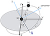 |
Fig. 1. Description of Keplerian orbits in terms of the orbital elements viewed in the fundamental reference frame (X,Y,Z). The Cartesian orbital frame (x,y,z) and the polar one |

where T0 is the proper time of periapsis passage4. In order to make contact with the literature, we then define

where  is the Einstein delay; in practice this term is presently indistinguishable from βb, which means that
  . Lastly, in this work we always ignore the Shapiro delay term in the timing model
With the timing model at hand we can perturbatively solve for N as a function of t and the timing-model parameters to obtain
where we defined the function

and a new eccentric anomaly E′ as
Eq. (7) defines the BT timing model, for which we can equivalently use the parameter sets  or
or  . On top of these, there are the parameters
  , ν,
, ν,  and
and  that are related to the pulsar’s own rotation (and are common to all timing models)
If the orbit is nearly circular, e → 0, T0 and ω are ill-defined because there is no periapsis. In this case we can define a different set of variables, the Laplace-Lagrange parameters η (not to be confused with parameter  defined in Eq. (6)) and κ, as


and we can replace T0 with Tasc, which stands for the time of ascending node. In analogy with the definition (5) we write
with  5. In order to make contact with the new eccentric anomaly E′ we can finally define a new variable Ψ′ through
With these parameters, the relationship (7) becomes
where now
Eq. (14) defines the ELL1 timing model Lange et al. (2001), that is, the set  or with
2.2. Ultra-light dark matter as a perturbing force
The unperturbed orbital motion of two bodies in the binary is completely characterised by six orbital parameters: a, e, ι, ω, T0 and the longitude of the ascending node Ω. The ULDM field  , owing to its interaction with the binary system, perturbs the system’s orbital motion and modifies the timing models of (7) or (14) that describe it. To illustrate our method, here we consider an effective, universal, direct linear coupling between the ULDM field and the two bodies in the binary system. The coupling is characterised by a single parameter α for which we can perturbatively write
where A ∈ {1, 2}, with M1 being the pulsar’s mass and M2 the mass of the companion6
The ULDM field can be considered homogeneous within its de Broglie wavelength (or coherence length), as determined by
where  is the typical ULDM velocity in the Milky Way halo. However, its amplitude and phase are expected to show large oscillations from binary system to binary system. Therefore, we describe the ULDM field as Foster et al. (2018)

where, assuming that each binary system is in a different coherence patch, Υ is a random phase with a flat distribution in [0, 2π) ,
the local ULDM density is taken to be ρDM = 0.3 GeV/cm3 and 𝜚 ≥ 0 is a random variable drawn from the Rayleigh distribution
The stochastic character of the ULDM field comes about because pulsar-timing observation campaigns typically last up to a few decades, which is a much shorter time than the ULDM coherence time
indeed, only by sampling the field during several  does the amplitude converge to
The perturbed, non-relativistic Keplerian equations of motion of a binary system interacting with ULDM are given by

where a dot denotes a derivative with respect to (coordinate) time, MT ≡ M1 + M2, R is the binary barycentre position defined using the unperturbed masses, r is the relative coordinate with origin in the companion body with mass M2 (readers can refer to Blas et al. 2020) that defines the polar coordinate system  ) of the orbital motion. In the last equality we defined F which we refer to as the ‘perturbing force’
2.3. Osculating orbits
The perturbing force F defined in Eq. (23) leads to deviations from the Kepler motion that can be studied using the osculating orbits formalism as described in Danby (1970). After some algebra (more in Appendix A), choosing {a , e , ω , ϵ1 , Ω , s} as the six independent orbital parameters, we obtain
![$$ \begin{aligned} \dot{\epsilon _1}&= \frac{2\alpha \Phi \omega _b}{1-e^2}(1+e\cos \theta ) \nonumber \\&\quad +\frac{2\alpha \dot{\Phi }e}{\sqrt{1-e^2}}\frac{r}{a}\sin \theta \nonumber \\&\quad +[1-\sqrt{1-e^2}]\dot{\omega } \,, \end{aligned} $$](/articles/aa/full_html/2024/10/aa49953-24/aa49953-24-eq46.gif)

where the parameter ϵ1 is given by
and is related to Θ′=Ψ′−ω by  .7 We note that scalar ULDM does not have any effect on the parameters ω and s, which we can henceforth discard. Integrating
  , using
  and allowing for a possible error and secular evolution of the semi-major axis
  , we find
![$$ \begin{aligned} \delta \Theta \prime&=\delta \Theta \prime _0 \nonumber \\&\quad +\int _{T_0}^{t}\left[\sqrt{\frac{G M_T(1+\alpha \Phi )}{(a+\delta a)^3}} -\sqrt{\frac{G M_T }{a ^3}}\right]\mathrm{d} t\prime \\&\quad +2\alpha \omega _b \int _{T_0}^t \Phi \, \mathrm{d} t\prime \nonumber \\&\quad +\alpha \sum _{n=1}^{\infty } \int _{T_0}^t \left[A_n \Phi \cos (n \omega _b \tilde{t}\prime )+ B_n \dot{\Phi }\sin (n \omega _b \tilde{t}\prime )\right]\, \mathrm{d} t\prime \nonumber \,, \end{aligned} $$](/articles/aa/full_html/2024/10/aa49953-24/aa49953-24-eq53.gif)
where δΘ′0 is the error in the determination of Θ′ at T0,  , with T0 = Tasc + ω/ωb, and
where  is a Bessel function of order n and
  its derivative with respect to its argument; in obtaining these expressions we have made use of the Fourier decomposition of the orbit, more in Appendix A
For orbits with small eccentricity that are described by the ELL1 model, at leading order in e → 0 the osculating orbit equations become

![$$ \begin{aligned} \frac{\dot{\eta }}{\eta } = \frac{\dot{\kappa }}{\kappa }&= -\frac{\alpha }{e} \left[\Phi \omega _b\sin \omega _b \tilde{t} + 2\dot{\Phi }\cos \omega _b\tilde{t}\right] \end{aligned} $$](/articles/aa/full_html/2024/10/aa49953-24/aa49953-24-eq60.gif)
Proceeding as with δΘ′, we find
![$$ \begin{aligned} \delta \Psi \prime&= \delta \Psi _{\rm asc}\prime \nonumber \\&\quad +\int _{T_{\rm asc}}^{t}\left[\sqrt{\frac{G M_T(1+\alpha \Phi )}{(a+\delta a)^3}} -\sqrt{\frac{G M_T }{a ^3}}\right] \mathrm{d} t\prime \nonumber \\&\quad + 2\alpha \omega _b\int _{T_{\rm asc}}^{t} \Phi \,\mathrm{d} t\prime \,. \end{aligned} $$](/articles/aa/full_html/2024/10/aa49953-24/aa49953-24-eq62.gif)
With Φ from Eq. (18), upon integration we find the expressions for the variations (denoted by δ) of the orbital parameters, which we collect in Appendix C
3. A two-step approach to estimate the sensitivity
Step 1: variances. In order to estimate the sensitivity to ULDM we follow the procedure outlined in Blandford & Teukolsky (1976), which we adapt to our needs by incorporating the Bayesian analysis of Moore et al. (2015). From Eq. (7) we see that the time-dependent function N is parametrised by N0, ν,  ,
,  and the orbital parameters, namely N = N(t, N0, ν, …). The first step is to assume that, for each binary system, we have a reasonable ‘first guess’ as to what the values of the orbital parameters are, which we denote {N0(1), ν(1), …}. This can be for instance obtained by fitting time-of-arrival data with the help of tools such as TEMPO2 Hobbs et al. (2006) or PINT Luo et al. (2021). We can then define the time residuals R(t) as

where N(t, N0, ν, …) corresponds to the observed time series (or a synthetic one with model parameters  ). Explicitly, the function R(t) reads
where
In order to simplify the notation below we define a vector  containing the model parameters of the residuals that can in principle be measured for both the BT and ELL1 timing models, namely
  and
and  , respectively. In what follows we neglect the contribution of the term with
  everywhere in Eq. (38) except in δK
We now assume that the observations are made at regular time intervals at a rate nc for a duration d such that Pb ≪ d ≪ Tobs where Tobs is the total time of observation. We also assume that each observation has a constant variance ϵ2 and zero covariance. In each interval of length d we minimise the χ2 for the ncd observations made in that interval and obtain an equation of the form
where the summation is over the number of observations, and we defined the vector D which contains the data. We then approximate the summation with its average times the number of observations as
where dΘ′ should be replaced by dΨ′ in the ELL1 model. Finally, the covariance matrix is obtained as

from where we can read off the variances for all the parameters that define the system–we collect these variances in Appendix B
Step 2: time-dependence. The second step consists of fitting the variances obtained in the first step to a time-dependent function which captures the evolution of the perturbations to the binary system. In Blandford & Teukolsky (1976) the time-evolution of the orbital parameters is assumed to be a polynomial up to the quadratic order. However, since we are seeking to detect the sinusoidal perturbation exerted by ULDM, we employ a Bayesian approach that mirrors the one for gravitational waves Moore et al. (2015)
We assume that the number of measurements 𝒩 = Tobs/d of the parameter set  is large and that they are regularly made within the observation time. For any of the parameters S for which a variance has been estimated in step 1, σS2 = var(δS) where
  , we define

![$$ \begin{aligned} \mathbf{h}(t)&\equiv \alpha \left[\mathbf{A}_X(t)X+\mathbf{A}_Y(t)Y\right]\,, \end{aligned} $$](/articles/aa/full_html/2024/10/aa49953-24/aa49953-24-eq80.gif)

here m and h are 𝒩-dimensional vectors that describe the model–we note that these vectors are not of the same dimensionality as the parameter sets  . The parameters Ξ0, Ξ1 and Ξ2 are the constants that define the quadratic fit of Blandford & Teukolsky (1976) (we note that some of the variables have Ξ2 = 0); n is the noise of the measurement, which is assumed to be white, Gaussian and uncorrelated between pulsars;
  is the signal caused by the presence of ULDM. For future convenience, here we have also separated the sinusoidal ULDM contribution into its
  and
and  contributions where
  and
and  8. For instance, in the ELL1 model, from Eq. (33) we find
![$$ \begin{aligned} \delta {x}(t)&= \delta {x}_{\rm asc}+\dot{x} (t-T_{\rm asc}) \nonumber \\&\quad -2 \alpha x \Phi _0 \varrho [\cos (m t+\Upsilon )-\cos (m T_{\rm asc}+\Upsilon )] \nonumber \\&= \Xi _0^x + \Xi _1^x t + h^x(t) \,,\end{aligned} $$](/articles/aa/full_html/2024/10/aa49953-24/aa49953-24-eq89.gif)
![$$ \begin{aligned} h^x(t)&= -2 \alpha x \Phi _0 \varrho [\cos (m t+\Upsilon )-\cos (m T_{\rm asc}+\Upsilon )]\,,\end{aligned} $$](/articles/aa/full_html/2024/10/aa49953-24/aa49953-24-eq90.gif)
![$$ \begin{aligned} A_X(t)&=-\sqrt{2} x \Phi _0 [\cos (m t)-\cos (m T_{\rm asc})]\nonumber \,,\\ A_Y(t)&=\sqrt{2} x \Phi _0 [\sin (m t)-\sin (m T_{\rm asc})]\,, \end{aligned} $$](/articles/aa/full_html/2024/10/aa49953-24/aa49953-24-eq91.gif)
where  in this case as there is no quadratic term–further explicit expressions for the variations
  can be found in Appendix C
The time-model for a given orbital parameter variation needs to be tested against an alternative model wherein there is no ULDM, namely  . We call these two competing models the signal and noise hypotheses, respectively. In order to account for our ignorance in the quadratic fitting parameters as well as the specific realisation of the local ULDM at the location of the pulsar, we marginalise over Ξj (which include possible secular variations of the orbital parameters) assuming uniform prior. Moreover, unless otherwise specified, we also use a uniform prior for the ULDM phase Υ, whereas for 𝜚 we use Eq. (20); thence, the probability distribution functions for the X and Y variables is given by
Lastly, the noise distribution can be written as
where Σn is a diagonal matrix with all diagonal elements identical to σS2, calculated in the first step
To compare the two hypotheses, the signal  and the noise
  for a given parameter S, we compute the ratio of the evidences 𝒪h and 𝒪n for the signal and the noise hypotheses, respectively. The evidences are defined as the likelihood marginalised over all the parameters of the model. The ratio of the evidences of the two models defines the Bayes factor ℬ as:

Explicitly, log-likelihoods for the signal and noise hypotheses are

where d is the 𝒩−dimensional vector that contains the data. Following Moore et al. (2015) we further define the matrices

where M is the so-called design matrix which admits a singular value decomposition into the matrices U (of dimension 𝒩 × 𝒩), T (of dimension 𝒩 × 3) and V (of dimension 3 × 3)–U is conveniently written in terms of F and G with G an 𝒩 × 𝒩 − 3 matrix9. From this decomposition the evidence for the noise hypothesis results in
In order to obtain the evidence for the signal hypothesis we need to assume priors for α and the mass m. If we adopt a stringent detection threshold (namely, a Bayes factor of 1000) we can assume that the posterior distributions for α and m are sufficiently peaked at the true values, and that the choice of any reasonable prior for them would not affect this. Therefore, since we are interested in evaluating the sensitivity curve for α as a function of m, we use a delta-function prior for α and m centred at their fiducial values αf and mf

Hence, the evidence for the signal hypothesis is given by
After performing the two trivial integrations over α and m, we are left with a number of gaussian integrals which can be computed straightforwardly, more in Appendix C
Finally, we average the Bayes factor over many realisations of the noise  . The result is

where in these quantities (their definition is in Appendix C) all the parameters are replaced by their fiducial values (i.e. α → αf, m → mf, 𝜚 → 𝜚f, and Υ → Υf). If instead of using P(X, Y) given in Eq. (51) we use delta-function priors also for X and Y (which is equivalent to assuming that we know the exact ULDM configuration for a given pulsar), we find  where
where 
At last, we can combine all binary pulsars by multiplying the Bayes factors as

where Np is the total number of binary pulsars,  corresponds to the p-th binary system for which the Bayes factors individually are given in Eq. (60). The constraint
  , which we call the sensitivity, is obtained by choosing a threshold value for detection, customarily set to be
readers can refer to Moore et al. (2015). For simplicity, in what follows, and in particular in Sects. 4 and 5, we drop the subscript ‘f’ for the fiducial values of α and m
4. Results
4.1. Near-circular orbits
As a first application of our method, we apply it to a set of 19 binary pulsars for which the orbital parameters were obtained by the NANOGrav collaboration Gabriella et al. (2023) using the ELL1 model and 3 binary pulsars modelled with the ELL1H (a variant on ELL1 which differs only in the parametrisation of the relativistic Shapiro time delay which we do not consider here Hobbs et al. (2006), Luo et al. (2021)) – we list the properties of all the binary pulsars that we use in this work in Tables E.1 and E.2. For each binary system we use the NANOGrav values of Tobs (MJD), ϵ and nc, and assume  . We note that, as we are forecasting the constraining power of data, and not running an actual data analysis, we need to assume the fiducial values for ϱ and Υ, or, equivalently, X and Y; in other words, we need to simulate our data vectors and with them the unknown values of the ULDM parameters; we do this by assigning separately to each binary system a random realisation of such parameters as taken from their corresponding theoretical distributions
In Fig. 2 we show the sensitivity obtained by applying Eq. (64) to the parameters  and
and  for ten different realisations of the fiducial ULDM model. In this figure we also show the current bounds obtained by Solar System constraints Bertotti et al. (2003) and Armstrong et al. (2003), and the bounds obtained with pulsar-timing arrays (PTAs) Porayko et al. (2018), Smarra et al. (2023). We see that, first of all, for a wide range of ULDM masses the sensitivity of binary pulsars supersedes the current Solar System constraints. This is mostly coming from the
  orbital parameter, which is by far more sensitive for small masses. The
  parameter, closely related to the semi-major axis a, is the more sensitive of the two at large ULDM masses, but it currently does not give a competitive constraint. However, current PTA searches provide the most stringent limits on α in the low-frequency regime, which are two to three orders of magnitude better than our limits
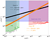 |
Fig. 2. Sensitivity of 22 near-circular binary pulsars, as measured by NANOGrav, to the coupling α as a function of the ULDM mass m. The sensitivities obtained from δx are in black, whereas those pertaining to |

Thanks to the near-analyticity of our model we can readily predict how much this result would improve for any given set of parameters of future observations. In Fig. 3 we combine 111 systems taken from the ATNF pulsar catalogue Manchester et al. (2005) and, based on the analysis presented in Liu et al. (2011) for a new generation of radio telescopes (e.g. the Square Kilometre Array, SKA), as an illustration of forecasting for such experiments we assume Tobs = 10 years, ϵ = 0.1 μs, nc = 1/ day. As we can see in the figure, the sensitivity in this case improves by well over an order of magnitude, bringing the binary pulsar constraint below the Solar System one for a larger range of ULDM masses. In particular, the sensitivity obtained with our method extends to masses beyond the Nyquist frequency of PTAs, and can beat Solar System tests in that range by up to one order of magnitude
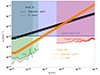 |
Fig. 3. Same as in Fig. 2 but using 111 binary pulsars from the ATNF catalogue and assuming next-generation radio-telescope precision. We assume Tobs = 10 years, and a next-generation radio-telescope precision given by ϵ = 0.1 μs (based on the analysis presented in Liu et al. (2011) for the upcoming SKA) |
In order to show how our results depend on the choice of priors for the ULDM parameters X and Y (corresponding to choices of ϱ and Υ), in Figs. 2 and 3 we also show the sensitivity curves for delta-function priors  and
and  . We observe that, while the choice of prior is not entirely negligible, nonetheless the effect is limited to a factor of order unity. Lastly, we note that the variations of the Laplace-Lagrange orbital parameters η and κ do exhibit resonances (as indicated in Eqs. (C.20) and (C.21)); however, beyond the resonant peak these parameters are less sensitive than x and
4.2. Resonances
When a system possesses a significant eccentricity e its orbital parameters experience resonant secular drifts Blas et al. (2017, 2020), and obtaining the sensitivity becomes much more computationally intensive. Therefore, here we limit ourselves to the effects of ULDM on Pb, and not the full variation of the parameter  defined in Eqs. (9) and (30) and refer to Appendix D for a more detailed discussion on this simplification, which does not appreciably alter our results. We call this contribution δΘ′Pb, defined as
With this proviso, in Figs. 4–6 we show the sensitivity obtained from this simplified  for the three binary pulsars J1946+3417, J2234+0611 and J1903+0327, respectively (we collect their parameters in Table E.2); as in Sect. 4.1 we run ten realisations of the ULDM parameters for each binary system
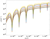 |
Fig. 4. Sensitivity to α as a function of ULDM mass m for ten realisations of the ULDM parameters 𝜚 and Υ, obtained from the binary pulsar J1946+3417 as measured by NANOGrav |
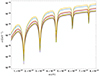 |
Fig. 5. Sensitivity to α as a function of ULDM mass m for ten realisations of the ULDM parameters 𝜚 and Υ, obtained from the binary pulsar J2234+0611 as measured by NANOGrav |
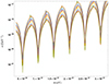 |
Fig. 6. Sensitivity to α as a function of ULDM mass m for ten realisations of the ULDM parameters 𝜚 and Υ, obtained from the binary pulsar J1903+0327 as measured by NANOGrav |
The combined sensitivity from all three systems, which beats each of them separately, as expected, is shown in Fig. 7. In these figures we limit ourselves to a smaller mass range to focus on the resonances, and we can see how these systems are in effect less constraining than the near-circular ones, their combined sensitivity approaching that of Solar System tests only for the most peaked resonances at low masses. Finally, the results of this section are directly comparable to Blas et al. (2020); we see that, while we reproduce these results very closely near the resonances, the off-resonance sensitivity as obtained from our method is in fact better than originally estimated
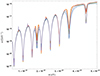 |
Fig. 7. Sensitivity to α as a function of ULDM mass m for five realisations of the ULDM parameters 𝜚 and Υ, obtained from the combination of the three binary pulsars J1946+3417, J2234+0611 and J1903+0327 as measured by NANOGrav |
5. Conclusion and outlook
Summary. In this paper we computed the sensitivity of binary pulsars for the detection of scalar ULDM for the entire mass range  , and for both eccentric and near-circular systems. We improve on previous results which only considered resonances between the systems’ orbital periods and ULDM oscillations by developing a method that goes beyond resonances. With the new method it is also possible to quantify our ignorance on the local DM field (i.e. the local amplitude determined by the parameter 𝜚 and the phase Υ). We find that, while our method is not competitive in the range of frequencies surveyed by PTAs, beyond the Nyquist frequency binary pulsars can be the most sensitive detectors for ULDM. For instance, we expect that observations made with the future SKA would be sensitive to ULDM couplings
  for
for  , better than Solar System constraints. In this regard, we notice that the most sensitive orbital parameter is
  (for ELL1 binaries) or
  (for BT binaries), highlighting the relevance of orbital parameters other than the most-studied (and often best-measured) orbital period
Relevance. Our results highlight why it is important to go beyond resonances. Firstly, resonances, being narrow resonances, are limited to a very narrow range of ULDM masses in correspondence with integer multiples of the binary system inverse period: going beyond resonances allows us to extend the sensitivity of each binary system to the entire mass range of interest, only limited by the binary pulsar back-reactions on the field Φ on the higher end Blas et al. (2020) and cosmological constraints on  on the lower end (readers can refer, for instance, to Shevchuk et al. (2023) and references therein). Secondly, in the scalar ULDM case resonances disappear for near-circular orbits; since near-circular orbits constitute the majority of binary pulsars in nature, for scalar ULDM searches we are limited to a minority of systems. Going beyond resonances means that each observed binary system contributes to the sensitivity for ULDM. Thirdly, each binary system contributes separately to the sensitivity to ULDM, as obtained from the secular orbital drifts caused by resonances. With our new method all binary pulsars jointly contribute to the sensitivity, thereby improving it across all masses
Context. Our findings should be compared with existing limits on scalar ULDM. We have already shown the limit coming from the Doppler tracking of the Cassini spacecraft, which results in  across all the masses we consider here Bertotti et al. (2003). Because a putative ULDM direct coupling α is equivalent to a scalar gravitational wave, the Cassini spacecraft also sets a constrain on the mass range
  that is about an order of magnitude stronger Armstrong et al. (2003). In the lowest frequency range considered in this work, current searches of the stochastic gravitational wave background by pulsar-timing arrays set the limits on ULDM around
  for a decade in mass around
  Porayko et al. (2018), Smarra et al. (2023). Furthermore the dynamical friction within the solitonic core of the ULDM halo changes the spectral slope of the stochastic background of gravitational waves which is at odds with what has been measured by pulsar-timing arrays, possibly implying the exclusion of ULDM masses within the range
  Aghaie et al. (2023). Existing limits also come from superradiance. By measuring the spin and mass of known black holes and other astrophysical objects, and assuming no interaction between Φ and standard matter, the mass ranges
  and
and  are excluded, or else these black holes and celestial objects would not be there Stott (2020). Therefore, the limits we obtain from binary pulsars at the same time constitute an independent test of some of the parameter space that is probed by superradiance, as well as a test of regions not accessible by it
Prospects. In this work we have concerned ourselves with the simplest case of a universally-coupled linear scalar ULDM field only. In the future we plan to investigate the spin-1 and spin-2 ULDM cases, for which only the resonant effects have been studied López Nacir & Urban (2018), Armaleo et al. (2020a). The main difference with respect to the scalar case is that, if ULDM has spin 1 or spin 2, even circular orbits experience resonant secular orbital drifts. Moreover, since the geometry of the ULDM perturbations on the orbital motion is different, we expect that it is possible to differentiate between different ULDM spins. The spin-2 case is especially interesting because ULDM with spin 2 mimics a continuous gravitational wave, albeit with five polarisations, readers can refer to Armaleo et al. (2021). Important extension to this work are the cases of a non-universal coupling as well as a quadratic coupling, which present distinctive phenomenology compared to the linear case–readers can refer, for instance, to Blas et al. (2020). Furthermore, a more detailed analysis would include other sources of noise (such as pulsar red noise) as well as more complex and complete timing models, which are optimally tailored to each binary pulsar system. Finally, we plan to empirically test our results by directly injecting a model ULDM signal to simulated binary pulsar time-of-arrival data, and then using different methods (applied to simulated data) in order to recover the injected ULDM signal within the predicted level of sensitivity
With the advent of the next generation of radio surveys such as the SKA we expect to observe an order-of-magnitude more binary pulsars than today. With our method it is immediate to combine all the systems, each with very different properties, into a single sensitivity curve across all relevant masses, and thus assess the chances for either ULDM detection, or the tightest constraints on its parameter space as new systems are discovered
The times of arrival of pulses of pulsars, whether isolated or in binary systems, are also directly sensitive to ULDM oscillations, a fact that can be exploited by pulsar-timing arrays Khmelnitsky & Rubakov (2014), Armaleo et al. (2020b)
Strictly speaking, t is not the time measured by an observer on Earth, but it corresponds to the so-called infinite-frequency barycentre arrival time which is a hypothetical time of arrival at the barycentre of the Solar System that includes corrections due to the motion of the Earth with respect to the barycentre, the gravitational redshift in the Solar System and the effect of interstellar dispersion (readers can refer to Blandford & Teukolsky (1976) for an introduction). Here we are assuming that such effects can be computed so that t is a known function of the arrival time at Earth
We note that here we use a different notation than in Blandford & Teukolsky (1976), namely Θ = σ + ∫0TωbdT′
We note that here we call Ψ to denote what is often called Φ in the literature (readers can refer, for instance, to Lange et al. (2001), Hobbs et al. (2006)), because in our notation Φ stands for the ULDM field
If the scalar theory is endowed with a, e.g.  symmetry, the first interaction term would be quadratic in the field Φ. We comment on this case in Sect. 5. We note that we also do not take into account non-perturbative effects such as scalarisation
The parameter ϵ1 is defined in Danby (1970) in order to avoid a term in the equation where t appears as a coefficient. Such a term could produce large quantities when evolving the equations for a long time
The matrix  is not to be confused with the matrix
  defined above in Eq. (41)
Acknowledgments
The Authors wish to thank Stéphane Ilić for useful discussion. DLN acknowledges support from ESIF and MEYS (Project ‘FZU researchers, technical and administrative staff mobility’ – CZ.02.2.69/0.0/0.0/18_053/0016627), UBA and CONICET. PK and FU acknowledge support from MEYS through the INTER-EXCELLENCE II, INTER-COST grant LUC23115. This article is based upon work from COST Action COSMIC WISPers CA21106, supported by COST (European Cooperation in Science and Technology)
References
- Aghaie, M., Armando, G., Dondarini, A., & Panci, P. 2023, Phys. Rev. D, 109, 103030 [Google Scholar]
- Armaleo, J. M., López Nacir, D., & Urban, F. R. 2020a, JCAP, 2001, 053 [CrossRef] [Google Scholar]
- Armaleo, J. M., López Nacir, D., & Urban, F. R. 2020b, JCAP, 09, 031 [CrossRef] [Google Scholar]
- Armaleo, J. M., López Nacir, D., & Urban, F. R. 2021, JCAP, 04, 053 [CrossRef] [Google Scholar]
- Armstrong, J. W., Iess, L., Tortora, P., & Bertotti, B. 2003, ApJ, 599, 806 [NASA ADS] [CrossRef] [Google Scholar]
- Bertotti, B., Iess, L., & Tortora, P. 2003, Nature, 425, 374 [Google Scholar]
- Blandford, R., & Teukolsky, S. A. 1976, ApJ, 205, 580 [Google Scholar]
- Blas, D., López Nacir, D., & Sibiryakov, S. 2017, Phys. Rev. Lett., 118, 261102 [NASA ADS] [CrossRef] [Google Scholar]
- Blas, D., López Nacir, D., & Sibiryakov, S. 2020, Phys. Rev. D, 101, 063016 [NASA ADS] [CrossRef] [Google Scholar]
- Damour, T., & Taylor, J. H. 1991, ApJ, 366, 501 [NASA ADS] [CrossRef] [Google Scholar]
- Danby, J. 1970, Fundamentals of Celestial Mechanics (MacMillan) [Google Scholar]
- Foster, J. W., Rodd, N. L., & Safdi, B. R. 2018, Phys. Rev. D, 97, 123006 [NASA ADS] [CrossRef] [Google Scholar]
- Gabriella, A., Md, Faisal A., Akash, A., et al. 2023, ApJ, 951, 78 [NASA ADS] [CrossRef] [Google Scholar]
- Hobbs, G., Edwards, R., & Manchester, R. 2006, MNRAS, 369, 655 [NASA ADS] [CrossRef] [Google Scholar]
- Khmelnitsky, A., & Rubakov, V. 2014, JCAP, 1402, 019 [CrossRef] [Google Scholar]
- Lange, C., Camilo, F., Wex, N., et al. 2001, MNRAS, 326, 274 [NASA ADS] [CrossRef] [Google Scholar]
- Liu, K., Verbiest, J. P. W., Kramer, M., et al. 2011, MNRAS, 417, 2916 [Google Scholar]
- López Nacir, D., & Urban, F. R. 2018, JCAP, 1810, 044 [CrossRef] [Google Scholar]
- Lorimer, D. R. 2008, Liv. Rev. Rel., 11, 8 [Google Scholar]
- Lorimer, D. R., & Kramer, M. 2004, Handbook of Pulsar Astronomy (Cambridge, UK: Cambridge University Press), 4, 2004 [Google Scholar]
- Luo, J., Ransom, S., Demorest, P., et al. 2021, ApJ, 911, 45 [NASA ADS] [CrossRef] [Google Scholar]
- Manchester, R. N., Hobbs, G. B., Teoh, A., & Hobbs, M. 2005, AJ, 129, 1993 [Google Scholar]
- Moore, C. J., Taylor, S. R., & Gair, J. R. 2015, CQG, 32, 055004 [NASA ADS] [CrossRef] [Google Scholar]
- Porayko, N. K., Zhu, X., Levin, Y., et al. 2018, Phys. Rev. D, 98, 102002 [NASA ADS] [CrossRef] [Google Scholar]
- Shevchuk, T., Kovetz, E. D., & Zitrin, A. 2023, ArXiv e-prints [arXiv:2308.14640] [Google Scholar]
- Shklovskii, I. S. 1970, Sov. Astron., 13, 562 [NASA ADS] [Google Scholar]
- Smarra, C., Goncharov, B., Barausse, E., et al. 2023, Phys. Rev. Lett., 131, 171001 [NASA ADS] [CrossRef] [Google Scholar]
- Stott, M. J. 2020, ArXiv e-prints [arXiv:2009.07206] [Google Scholar]
- Turner, M. S. 1979, ApJ, 233, 685 [NASA ADS] [CrossRef] [Google Scholar]
- Watson, G. 1995, A Treatise on the Theory of Bessel Functions, Cambridge Mathematical Library (Cambridge University Press) [Google Scholar]
Appendix A: Post-Keplerian orbits
The orbital parameters of a perturbed binary system evolve with time according to the equations Turner (1979), Danby (1970),
![$$ \begin{aligned} \dot{\varpi }&= \frac{\sqrt{1-e^2}}{a e\omega _b} \left\{ -F_{r} \cos \theta +F_{\theta }\sin \theta \left[1+\frac{r}{a(1-e^2)}\right]\right\} + 2\sin ^2\left(\frac{\iota }{2}\right)\dot{\Omega }\,, \end{aligned} $$](/articles/aa/full_html/2024/10/aa49953-24/aa49953-24-eq152.gif)
![$$ \begin{aligned} \dot{\epsilon }_1&= -\frac{2rF_{r}}{a^2\omega _b}+\left[1\!-\!\sqrt{1-e^2}\right] \dot{\varpi }+ 2\sqrt{1-e^2} \sin ^2\left(\frac{\iota }{2}\right) \dot{\Omega }\,, \end{aligned} $$](/articles/aa/full_html/2024/10/aa49953-24/aa49953-24-eq153.gif)
where

is the binary orbital frequency and we have decomposed the perturbing force in the cylindric coordinates,
In Eqs. (A.5) and (A.6) we have introduced the argument of the pericentre,

and the parameter
The orbital motion for elliptic orbits is not expressible in closed form, but can be represented as Fourier decomposition of combinations of the unperturbed Keplerian orbits, which amounts to a harmonic expansion in eccentricities Watson (1995):

where  , Jn(z) is a Bessel function of order n and Jn′(z) is its derivative with respect to z
Appendix B: Variances
B.1. Elliptic orbits
The time residual for the BT model is given by Eq. (38) in terms of six independent parameters:  . The dependence on δa only comes from the dependence on ωb in the last term of Eq. (7), which is a subdominant contribution with respect to the other terms. Here, for simplicity, we follow Blandford & Teukolsky (1976) and we neglect such contribution to estimate the variances of the remaining five parameters:
  . The dominant part of the time residual can be written as
![$$ \begin{aligned} R^{\mathrm{BT} }&= \, \delta \eta _b \sin E^{\prime }- \delta e \left[\alpha _b +\frac{\sin E^{\prime } \left(\alpha _b \sin E^{\prime }-\eta _b \cos E^{\prime }\right)}{1-e \cos E^{\prime }}\right]+\delta \alpha _b \left(\cos E^{\prime }-e\right)\nonumber \\&-\frac{\delta \Theta ^{\prime } \left(\alpha _b \sin E^{\prime }-\eta _b \cos E^{\prime }\right)}{1-e \cos E^{\prime }} \,, \end{aligned} $$](/articles/aa/full_html/2024/10/aa49953-24/aa49953-24-eq169.gif)
and the variances for the parameters for generic values of e, αb and ηb are as follows
![$$ \begin{aligned} \mathrm{var} ({\delta K})&= -\mathcal{Q} \left\{ \eta _b^4 \left[e^4 (26-9 \varepsilon )+4 e^2 (8 \varepsilon -7)+8 (\varepsilon -1)\right] \right. \nonumber \\&+2 \alpha _b^2 \eta _b^2 \left[e^6+e^4 (18-5\varepsilon )+4 e^2 (6 \varepsilon -5) +8 (\varepsilon -1)\right] \nonumber \\&+\alpha _b^4 \left[8 e^8+e^6 (32 \varepsilon -62)+e^4 (74-65 \varepsilon )+4 e^2 (4\varepsilon -3)+8 (\varepsilon -1)\right]\left.\right\} \,,\end{aligned} $$](/articles/aa/full_html/2024/10/aa49953-24/aa49953-24-eq170.gif)
![$$ \begin{aligned} \mathrm{var} ({\delta \alpha _b})&= \,\mathcal{Q} \left\{ 4\eta _b^4 \left[e^2 (\varepsilon -3)-4 \varepsilon +4\right] +2 \alpha _b^2 \eta _b^2 \left[7 e^4-22 e^2-2 \left(e^4-7 e^2+8\right) \varepsilon +16\right] \right. \nonumber \\&+\alpha _b^4 \left[e^6 (\varepsilon -6)+e^4 (30-16 \varepsilon )+8 e^2 (4 \varepsilon -5)-16 (\varepsilon -1)\right] \left.\right\} \,,\end{aligned} $$](/articles/aa/full_html/2024/10/aa49953-24/aa49953-24-eq171.gif)
![$$ \begin{aligned} \mathrm{var} ({\delta \eta _b})&= \,\mathcal{Q} \left\{ 4\alpha _b^4 \left(e^2-1\right)^2 \left[e^2 (\varepsilon -3)-4 \varepsilon +4\right] +2 \eta _b^4 \left[e^4+4 e^2 (\varepsilon -2)-8\varepsilon +8\right] \right. \nonumber \\&+\alpha _b^2 \eta _b^2 \left[e^6 (\varepsilon -6)+e^4 (42-20 \varepsilon )+e^2 (52 \varepsilon -68)-32 (\varepsilon -1)\right] \left.\right\} \,,\end{aligned} $$](/articles/aa/full_html/2024/10/aa49953-24/aa49953-24-eq172.gif)
![$$ \begin{aligned} \mathrm{var} ({\delta e})&= \,\mathcal{Q} e^4 \left\{ \alpha _b^2 \left(e^2-2\right) \left[e^2 (\varepsilon -2)-2 \varepsilon +2\right]-2 \eta _b^2 \left(e^2+2 \varepsilon -2\right)\right\} \,,\end{aligned} $$](/articles/aa/full_html/2024/10/aa49953-24/aa49953-24-eq173.gif)
![$$ \begin{aligned} \mathrm{var} ({\delta \Theta ^{\prime }})&= \,\mathcal{Q} \varepsilon e^2 \left\{ 2 \alpha _b^2 \left(e^2-1\right) \left[e^2 (\varepsilon -2)-2 \varepsilon +2\right]+\eta _b^2 \left(e^2-2\right) \left(e^2+2 \varepsilon -2\right)\right\} \,, \end{aligned} $$](/articles/aa/full_html/2024/10/aa49953-24/aa49953-24-eq174.gif)
where
![$$ \begin{aligned} \mathcal{Q} \equiv \frac{\epsilon ^2}{d n_c \left[e^4+4 e^2 (\varepsilon -2)-8 \varepsilon +8\right] \left[\eta _b^2-\alpha _b^2 \left(e^2-1\right)\right]^2} \,, \end{aligned} $$](/articles/aa/full_html/2024/10/aa49953-24/aa49953-24-eq175.gif)
and 
B.2. Near-circular orbits
In the ELL1 timing model it is not difficult to obtain an analytic estimate for the variance of the six orbital parameters. These expressions are however very long and not illuminating, and for simplicity here we only quote the results for η ≃ κ ≃ 0
These expressions can be further simplified by noticing that the quantity
is very small, so that at leading order we have:
We note that the variances of δs and δκ are relatively large since powers of the small quantity xωb appear in the denominator. This is expected because the dependence on s only enters in the factor ωb in the last term of Eq. (14), which (as in the BT model) is a subdominant contribution. By ignoring such contribution the calculation of the variances of the remaining five independent parameters yields:
Therefore, except for δκ, this relatively simpler calculation gives similar results. The reason why the variance of δκ becomes smaller by neglecting the contribution of δs is that at leading (non-vanishing) order in xωb the term with δs, which is suppressed by xωb, becomes completely degenerate with the one with δκ (they have the same time dependence given by sin2Ψ′), which does not vanish for xωb → 0. It is only after including the  correction in xωb for δκ that those parameters can be distinguished
Appendix C: Bayesian approach
C.1. Perturbed BT model
The model for the variations of the orbital parameters for eccentric orbits including the ULDM contribution is given by:
![$$ \begin{aligned} \delta \Theta ^{\prime }(t)&= \delta \Theta ^{\prime }_0+ \frac{5}{2}\alpha \omega _b\frac{\Phi _0\varrho }{m}[\sin (mt+\Upsilon )-\sin (m T_0+\Upsilon )]+\alpha \Phi _0\varrho \sum _{n=1}^{+\infty } B_n \sin (n\omega _b\tilde{t})\cos (m t+\Upsilon ) \,\nonumber \\&+\alpha \frac{\Phi _0\varrho }{2}\sum _{n=1}^{+\infty } (A_n-n\omega _b B_n)\left\{ \frac{ \sin (m t+\Upsilon +n\omega _b\tilde{t})-\sin (m T_0+\Upsilon ) }{m+n\omega _b}\right.\nonumber \\&\left.+\frac{ \sin (m t+\Upsilon -n\omega _b\tilde{t})-\sin (m T_0+\Upsilon ) }{m-n\omega _b}\right\} -\frac{3}{2}\omega _b\int _{T_0}^t\frac{\delta a(t^{\prime })}{a} dt^{\prime }\,,\end{aligned} $$](/articles/aa/full_html/2024/10/aa49953-24/aa49953-24-eq187.gif)
![$$ \begin{aligned} \frac{\delta a(t)}{a}&= \frac{\delta a_0}{a}+\frac{\dot{a}_0\tilde{t}}{a}-2\alpha \Phi _0 \varrho [\cos (m t+ \Upsilon )-\cos (m T_0+ \Upsilon )]\nonumber \\&-8 \alpha \Phi _0 \varrho \sum _{n=1}^{+\infty } J_n(ne) [\cos (mt+\Upsilon )\cos (n\omega _b\tilde{t})-\cos (m T_0+\Upsilon )]\nonumber \\&+6 \alpha \Phi _0 \varrho \omega _b \sum _{n=1}^{+\infty } n J_n(ne)\left\{ \frac{\cos (m t+\Upsilon +n\omega _b\tilde{t})-\cos (m T_0+\Upsilon )}{m+n\omega _b }\right.\nonumber \\&\left.- \frac{\cos (m t+\Upsilon -n\omega _b\tilde{t})-\cos (m T_0+\Upsilon )}{m-n\omega _b } \right\} \,,\end{aligned} $$](/articles/aa/full_html/2024/10/aa49953-24/aa49953-24-eq188.gif)
![$$ \begin{aligned} \delta e(t)&= \delta e_0+\dot{e}_0\tilde{t}+\alpha \Phi _0 \varrho \frac{1-e^2}{e}\sum _{n=1}^{+\infty } J_n(ne) \left\{ \frac{n\omega _b-2m}{ n\omega _b+m}[\cos (m t+\Upsilon +n\omega _b \tilde{t})-\cos (m T_0+\Upsilon )]\right.\nonumber \\&\left.+\frac{2m+n\omega _b}{n\omega _b-m}[\cos (m t+\Upsilon -n\omega _b \tilde{t})-\cos (m T_0+\Upsilon )]\right\} \, ,\end{aligned} $$](/articles/aa/full_html/2024/10/aa49953-24/aa49953-24-eq189.gif)
![$$ \begin{aligned} \delta \omega (t)&= \delta \omega _0+\dot{\omega }_0\tilde{t}+\alpha \Phi _0 \varrho \frac{\sqrt{1-e^2}}{e} \sum _{n=1}^{+\infty }J_n^{\prime }(ne) \left\{ \frac{n\omega _b-2m}{ n\omega _b+m}[ \sin (m t+\Upsilon +n\omega _b \tilde{t})-\sin (m T_0+\Upsilon )] \right.\nonumber \\&\left.-\frac{2m+n\omega _b}{n\omega _b-m} [\sin (m t+\Upsilon -n\omega _b \tilde{t})-\sin (m T_0+\Upsilon )] \right\} \,, \end{aligned} $$](/articles/aa/full_html/2024/10/aa49953-24/aa49953-24-eq190.gif)
where  , An and Bn are defined in Eq. (31),
  ,
,  and
and  account for a constant shift due to the error in the determination of the parameters evaluated at T0, and the derivatives of the orbital parameters on the right-hand side account for the possibility of having another perturbation to the system (on top of the ULDM effect) which produces a secular variation. The variations
  and
and  do not have contributions from ULDM. We note that in the two-step approach presented in the main text we marginalise over those errors for each variable; we can therefore discard ULDM-dependent terms that can be absorbed in the errors of the orbital parameters, since the ULDM contribution cannot be determined separately
For the sake of completeness we write below the ULDM contribution decomposed into its X and Y components:
![$$ \begin{aligned} h^S(t)&\equiv&\alpha \left[ A_{X}^S(t)X+A_{Y}^S(t) Y\right]\,,\end{aligned} $$](/articles/aa/full_html/2024/10/aa49953-24/aa49953-24-eq198.gif)

![$$ \begin{aligned} \ell ^S(t)&\equiv&\alpha \left[L_{X}^S(t)X+L_{Y}^S(t)Y\right]\,, \end{aligned} $$](/articles/aa/full_html/2024/10/aa49953-24/aa49953-24-eq201.gif)
where hS(t) is the characteristic signals caused by ULDM on the variables δS that enter the likelihood in Eq. (54), for the BT model Tref = T0,
![$$ \begin{aligned} H^{\Theta ^{\prime }}_{P_b,X}(t)&= -\frac{ \Phi _0 \omega _b}{2^{3/2}}\left\{ \frac{-7 \sin m t }{m} + \sum _{n=1}^{+\infty }\frac{6 J_n(n e)}{(n \omega _b-m) (m+ n\omega _b)}\right.\nonumber \\&\times \left[ \frac{(m-n \omega _b) (2 m- n\omega _b) \sin (m t+t n \omega _b-T_0 n\omega _b )}{m+ n\omega _b}\right. \nonumber \\&+ \left.\left. \frac{(m+ n\omega _b) (2 m+ n\omega _b) \sin (m t-t n \omega _b+T_0 n\omega _b )}{m-n \omega _b}\right]\right\} \,,\end{aligned} $$](/articles/aa/full_html/2024/10/aa49953-24/aa49953-24-eq204.gif)
![$$ \begin{aligned} H^{\Theta ^{\prime }}_{P_b,Y}(t)&= -\frac{ \Phi _0 \omega _b}{2^{3/2}}\left\{ \frac{-7 \cos m t }{m} + \sum _{n=1}^{+\infty }\frac{6 J_n(n e)}{(n \omega _b-m) (m+ n\omega _b)}\right.\nonumber \\&\times \left[ \frac{(m-n \omega _b) (2 m- n\omega _b) \cos (m t+t n \omega _b-T_0 n\omega _b )}{m+ n\omega _b}\right. \nonumber \\&+ \left.\left. \frac{(m+ n\omega _b) (2 m+ n\omega _b) \cos (m t-t n \omega _b+T_0 n\omega _b )}{m-n \omega _b}\right]\right\} \,, \end{aligned} $$](/articles/aa/full_html/2024/10/aa49953-24/aa49953-24-eq205.gif)


for a, e and ω, the ℓS(t) contributions vanish while ℓΘ′(t) involves a linearly growing term
As already mentioned, in the two-step approach, in the definition of hS(t) a constant and a term that is linearly growing (in time) are irrelevant since they can be absorbed into a redefinition of the nuisance parameters. The reason we keep the constant terms in hS(t) (given by HXS(Tref) and HXS(Tref)) is because some variations present resonances and the constant parts are needed to obtain finite results at the resonance points
C.2. Perturbed ELL1 model
The model for the variations of the orbital parameters for near-circular orbits including the ULDM contribution is given by:
![$$ \begin{aligned} \delta \Psi ^{\prime }(t)&= \delta \Psi ^{\prime }_{\rm asc}-\frac{3\omega _b}{2}\left(\frac{\delta a_{\rm asc}}{a}+2 \alpha \Phi _0 \varrho \cos (m T_{\rm asc}+\Upsilon ) \right)\bar{t}-\frac{3\omega _b}{4}\frac{\dot{a}_{\rm asc} }{a}\bar{t}^2 \nonumber \\&+\frac{11\omega _b}{2 m}\alpha \Phi _0 \varrho \left[\sin (m t+\Upsilon )-\sin (m T_{\rm asc}+\Upsilon )\right] \,, \end{aligned} $$](/articles/aa/full_html/2024/10/aa49953-24/aa49953-24-eq213.gif)
![$$ \begin{aligned} \delta {x}(t)&= \delta {x}_{\rm asc}+\dot{x}_{\rm asc} \bar{t}-2 \alpha x \Phi _0 \varrho [\cos (m t+\Upsilon )-\cos (m T_{\rm asc}+\Upsilon )] \,, \end{aligned} $$](/articles/aa/full_html/2024/10/aa49953-24/aa49953-24-eq214.gif)
![$$ \begin{aligned} \delta {\kappa }(t)&= \delta {\kappa }_{\rm asc}+ \dot{\kappa }_{\rm asc} \bar{t} + \alpha \Phi _0 \varrho \frac{\kappa }{\kappa ^2+\eta ^2} \left\{ \frac{\kappa (\omega _b+2 m)}{2(\omega _b-m)}\left[ \cos (m t-\omega _b\bar{t} + \Upsilon ) -\cos (m T_{\rm asc} + \Upsilon ) \right] \right.\, \nonumber \\&+\left. \frac{\kappa (\omega _b-2 m)}{2(\omega _b+m)}\left[ \cos (m t+\omega _b\bar{t} + \Upsilon ) -\cos (m T_{\rm asc} + \Upsilon ) \right] - \frac{\eta (\omega _b+2 m)}{2(\omega _b-m)}\left[ \sin (m t-\omega _b\bar{t} + \Upsilon ) \right.\right.\nonumber \\&-\left.\left.\sin (m T_{\rm asc} + \Upsilon ) \right]+ \frac{\eta (\omega _b-2 m)}{2(\omega _b+m)}\left[ \sin (m t+\omega _b\bar{t} + \Upsilon ) -\sin (m T_{\rm asc} + \Upsilon ) \right] \right\} \,, \end{aligned} $$](/articles/aa/full_html/2024/10/aa49953-24/aa49953-24-eq215.gif)
![$$ \begin{aligned} \delta {\eta }(t)&= \delta {\eta }_{\rm asc}+ \dot{\eta }_{\rm asc} \bar{t} + \alpha \Phi _0 \varrho \frac{\eta }{\kappa ^2+\eta ^2} \left\{ \frac{\kappa (\omega _b+2 m)}{2(\omega _b-m)}\left[ \cos (m t-\omega _b\bar{t} + \Upsilon ) -\cos (m T_{\rm asc} + \Upsilon ) \right] \right.\, \nonumber \\&+\left. \frac{\kappa (\omega _b-2 m)}{2(\omega _b+m)}\left[ \cos (m t+\omega _b\bar{t} + \Upsilon ) -\cos (m T_{\rm asc} + \Upsilon ) \right] - \frac{\eta (\omega _b+2 m)}{2(\omega _b-m)}\left[ \sin (m t-\omega _b\bar{t} + \Upsilon ) \right.\right.\nonumber \\&-\left.\left.\sin (m T_{\rm asc} + \Upsilon ) \right]+ \frac{\eta (\omega _b-2 m)}{2(\omega _b+m)}\left[ \sin (m t+\omega _b\bar{t} + \Upsilon ) -\sin (m T_{\rm asc} + \Upsilon ) \right] \right\} \,, \end{aligned} $$](/articles/aa/full_html/2024/10/aa49953-24/aa49953-24-eq216.gif)
where  , the quantities
  ,
,  ,
,  and
and  account for possible errors evaluated at
  and, as for the BT model, possible secular variations due to other effects are also included in the model. The corresponding X and Y components defined in Eq. (C.2), where Tref = Tasc in the ELL1 model, are given by


![$$ \begin{aligned} H^\kappa _X(t)&= \frac{ \Phi _0 \kappa }{2^{3/2}(\kappa ^2+\eta ^2)} \left\{ \frac{ (\omega _b+2 m)}{(\omega _b-m)}\left[ \kappa \cos (m t-\omega _b\bar{t} ) - \eta \sin (m t-\omega _b\bar{t} ) \right] \right. \nonumber \\&+ \left. \frac{ (\omega _b-2 m)}{(\omega _b+m)}\left[ \kappa \cos (m t+\omega _b\bar{t} ) + \eta \sin (m t+\omega _b\bar{t} ) \right] \right\} \,,\end{aligned} $$](/articles/aa/full_html/2024/10/aa49953-24/aa49953-24-eq225.gif)
![$$ \begin{aligned} H^\kappa _Y(t)&= \frac{ \Phi _0 \kappa }{2^{3/2}(\kappa ^2+\eta ^2)} \left\{ \frac{- (\omega _b+2 m)}{(\omega _b-m)}\left[ \eta \cos (m t-\omega _b\bar{t} ) +\kappa \sin (m t-\omega _b\bar{t} ) \right] \right. \nonumber \\&+\left.\frac{ (\omega _b-2 m)}{(\omega _b+m)}\left[ \eta \cos (m t+\omega _b\bar{t} ) - \kappa \sin (m t+\omega _b\bar{t} ) \right] \right\} \,,\end{aligned} $$](/articles/aa/full_html/2024/10/aa49953-24/aa49953-24-eq226.gif)
The linear terms for x, κ and η, are zero, ℓS = 0, while for Ψ′ we have

We note that the signals for the parameters η and κ exhibit a resonant term, which comes from the first resonance  and is the only one that survives in the e → 0 limit
C.3. Integrals for marginalisation
The integral expression for the quantities needed to evaluate the Bayes’ factor ℬ are:
where all quantities are fixed to their fiducial values and for a given function of time f(t),
where mS = 0 if Ξ2 ≠ 0, mS = 1 if Ξ2 = 0 and Ξ1 ≠ 0, and mS = 2 if Ξ2 = 0 = Ξ1 and only Ξ0 ≠ 0
Appendix D: Resonances: going beyond Pb in the BT model
In this appendix we discuss on the importance of taking into account the ULDM effect on orbital parameters other than the orbital period Pb (which is the most studied one) for eccentric systems. We focus here on system J1903+0327, whose parameters are given in Table E.2, and compute the sensitivity curves using the effect of ULDM on the orbital parameter Θ′. The variance of δΘ′ is given in Eq. (B.6) while the model can be computed from Eq. (C.1a) where An and Bn are defined in Eq. (31)
Upon using Eq. (C.1b) into Eq. (C.1a) we can write δΘ′ as
where we have used the fact that
and we have included the parameter  in order to describe all possible secular variations that are not caused by ULDM (e.g. the Shklovskii effect Shklovskii (1970) or the galactic acceleration Damour & Taylor (1991)). Here we collect in Ξ0 all the constant contributions to δΘ′, regardless of whether these come from ULDM or some other effects; all the contributions growing linearly with t are included in the Ξ1t term. The relevant ULDM signal is characterised by the functions hΘ′(t) and hPbΘ′(t) given in Appendix C as
![$$ \begin{aligned} h^{\Theta ^{\prime }}(t)&= \alpha [( H_{X}^{\Theta ^{\prime }}(t)- H_{X}^{\Theta ^{\prime }}(T_0))X+( H_{Y}^{\Theta ^{\prime }}(t)- H_{Y}^{\Theta ^{\prime }}(T_0)) Y]\,,\end{aligned} $$](/articles/aa/full_html/2024/10/aa49953-24/aa49953-24-eq237.gif)
![$$ \begin{aligned} h^{\Theta ^{\prime }}_{P_b}(t)&= \alpha [( H_{P_b,X}^{\Theta ^{\prime }}(t)- H_{P_b,X}^{\Theta ^{\prime }}(T_0))X+( H_{P_b,Y}^{\Theta ^{\prime }}(t)- H_{P_b,Y}^{\Theta ^{\prime }}(T_0)) Y]\,, \end{aligned} $$](/articles/aa/full_html/2024/10/aa49953-24/aa49953-24-eq238.gif)
where the functions on the right-hand-side are defined in Eq. (C.7). Here hΘ′(t) describes the effect of ULDM on Θ′ given in Eq. (C.1a) and hPbΘ′(t) takes into account only the ULDM effect on Pb obtained from the last term in Eq. (C.1a) and Eq. (D.2)
We note that the constant parameters Ξ0 includes the error in the determination of Θ′0, and the coefficient Ξ1 of the linear term depends on the error in the determination of a0. In order to obtain the sensitivity curve for α, we use the variance of δΘ′ given in Eq. (B.6) and marginalise over the two nuisance parameters Ξ0 and Ξ1 in the model of Θ′ using uniform priors for both of them. We assume here that any possible secular effect on Pb characterised by  in Eq. (D.1) can be independently determined with significant precision so that we can subtract them and then set
  (more in Appendix E where we show that this simplification is only relevant for masses that are very close to the resonance; this is the case because ULDM produces a secular effect at m = nωb, but not for other values of the mass)
In order to illustrate the difference in sensitivity that could be obtained by performing an analysis with hΘ′(t) in comparison to hPbΘ′(t), we restrict ourselves to the study of the signal at low masses, where the contribution of the first harmonic with n = 1 in Eq. (C.1a) dominates the signal and accounts for a resonant effect for m = ωb. Within the scope of this work it is enough to focus on the contribution of the first n = 1 harmonic, so we neglect higher ones. The result is shown in Fig. (D.1), where we plotted the sensitivity curves for five different random realisations of the values of 𝜚 and Υ, for which we used different colours. The dashed lines were obtained using hΘ′(t) while the solid lines correspond to hPbΘ′(t). We see the effect on Pb dominates, so the estimated sensitivity obtained from both hPbΘ′(t) and hΘ′(t) are about the same. The use of hPbΘ′(t) instead of hΘ′(t) underestimate (overestimate) the sensitivity at the lower (higher) masses away from the resonant band but only by an order one factor
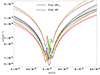 |
Fig. D.1. Sensitivity curves for α as a function of the ULDM mass m for the system J1903+0327 (with parameters given in Table E.2) for masses near the resonant one at ωb = m. Dashed lines account for all the ULDM effects on the parameter Θ′, while the solid lines are obtained neglecting the ULDM effect on all parameters but Pb. Each colour corresponds to a particular random realisation of the parameters 𝜚 and Υ |
Appendix E: Marginalisation and the resonant peaks in the two-step approach
In this appendix we analyse the sensitivity curves near the resonances. To this end, we consider the effect on δΘ′ at low masses around the first resonant peak m = ωb and neglect higher harmonics. For the sake of generality, we model the signal for the second step as

where hΘ′(t) and ℓΘ′(t) are defined as in Eq. (C.2) and are given in Eqs. (D.3) and (C.17), respectively. Here the parameters Ξi (i = 0, 1, 2) do not include the linear function in time coming from the ULDM contribution, which is given by ℓΘ′(t), nor the secular quadratic term that shows up at the resonant mass
Fig. E.1 shows the sensitivity curves as a function of the mass for the system J1903+0327 around the resonant mass m = ωb for five realisations of the parameters 𝜚 and Υ. Firstly, we see that the shape of the curve around the resonant mass depends strongly on the values of the parameters 𝜚 and Υ. Secondly, since we do not know the nuisance parameters Ξi (i = 0, 1, 2), an appropriate procedure to obtain a conservative sensitivity curve for α is to marginalise over such irrelevant parameters. However, in Fig. E.1 it can be seen that the differences between marginalising over the nuisance parameters, or neglecting them, are significant only in a tiny mass range near resonance.10 This is as expected, because only close to the resonance the ULDM produces a secular drift of the orbital period which can be swept in the marginalisation of the quadratic term Ξ2
22 pulsars described by the ELL1(H) model
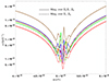 |
Fig. E.1. Sensitivity curves for α as a function of the ULDM mass m for the system J1903+0327 (with parameters given in Table E.2) for masses near the resonant one at ωb = m. Solid lines are obtained after marginalising over all the three nuisance parameters Ξi (i = 0, 1, 2) in the model of Θ′ (we use uniform priors for all of them), dashed lines are obtained after marginalising only over the parameters Ξ0 and Ξ1 (which correspond to a linear growth coefficient and a constant error in Θ′) while the coefficient Ξ2 (which gives a quadratic growth) is assumed to be known and subtracted so that Ξ2 = 0 |
Three pulsars with notably high eccentricity parametrised by the BT timing model
Appendix F: A one-step approach to estimate the sensitivity (cross-verification)
In this section we fit time residuals directly to the timing model (one-step approach) in order to construct the sensitivity curves. This approach is based on less robust assumptions, in particular we assume here that time residuals are due solely to the effect of ULDM on the binary’s orbital parameters and are subject to a Gaussian (white) noise distribution. We focus our analysis on the 22 ELL1(H) pulsars included in the NANOGrav 2023 dataset (we refer to Table E.1) and then extend this analysis to the three binary pulsars with higher eccentricity of Table E.2
Disadvantages. In the two-step approach we have introduced nuisance parameters to model possible errors or constant shifts in the determination of the orbital parameters and secular drifts from other sources, over which we have marginalised. The one-step method we describe here does not take into account any effect other than ULDM and noise, i.e. no such errors and secular drifts are included. Consequently, the sensitivity curves produced by this approach tend to be more optimistic (or less conservative) compared to those derived from the two-step method
Advantages. This method allows us to jointly consider variations of all orbital parameters, enhancing sensitivity—a capability lacking in the previous method. The marginalisation over 𝜚 and Υ using a Gaussian prior can be done fully analytically, giving insight into how the sensitivity depends on each variable such as observation time, noise magnitude, or cadence. Importantly, plotting the sensitivity curves is not time consuming, compared to the two-step method. Lastly, since not all binary pulsars are of the same quality in terms of their ability to detect ULDM, this method can be used to quickly determine which pulsars are the most suitable to study ULDM, allowing us to restrict ourselves to a selected subset of pulsars. This knowledge can be further exploited when using the two-step method
Timing model
In line with our assumptions, we decompose time residual R into two components
Here, RDM represents the contribution of ULDM in the ELL1 model, while RPN accounts for pulsar noise. Within the ELL1 model given in Eq. (39), at leading order in the small quantities η, κ, xωb and  , the variation of δx, δΨ′,δη, δκ leads to the following expression for the time residual RELL1

while RELL1 transforms into RDM when δx, δΨ′,δη, δκ arise from ULDM, given by Eq. (C.18). Since we are assuming here that the variations only come from the ULDM, in such perturbation we set to zero both the error and the derivative of the orbital parameters at Tasc, i.e. δx = hx etc
We note that the function δΨ′(t) given in Eq. (C.18) includes a constant term and a linear term (in time) that depend on the ULDM field, while the ULDM signal considered in the two-step method, namely hΨ′(t) defined in Eq. (C.2), does not incorporate those contributions, since they have been absorbed into the nuisance parameters. The presence of the linear term significantly enhances the sensitivity, but the result should be taken with a grain of salt because it assumes that other linear contributions are either subdominant or can be independently measured and subtracted away, whereas we expect that it is indistinguishable from an error in the semi-major axis  . Nonetheless, in order to understand the physical effect of the linear term, we present the sensitivity plots using the one-step method both with the presence of the linear term and without it. The sensitivity curves obtained in this section (without the linear term) become very close to the ones obtained from the two-step method
Noise model
Since we have already described dark matter component (we refer, for instance, to Appendix C), let us turn our attention to the noise model. We consider uncorrelated white Gaussian noise with correlation matrix
where  are pulsar indices and
  are TOAs indices, ϵa is the noise amplitude of pulsar a and the δs are Kronecker deltas
Concentrating on a single pulsar a, the likelihood function Pa of time residuals, denoted as {Ri}a, where curly brackets denote a set in which i = 1, …, na, with parameters pa ≡ (α,𝜚a,Υa) is
![$$ \begin{aligned} P_a\left( \{R_{i}\}_a | p_a \right) = \frac{1}{ (2\pi )^{\frac{n_a}{2} }\epsilon _a^{n_a}} \exp \left[ - \frac{1}{2} \sum _{i=1}^{n_a} \frac{\left( R_{ai} - R_{ai}^{\mathrm{DM} } \right)^2}{\epsilon _a^2} \right] \,. \end{aligned} $$](/articles/aa/full_html/2024/10/aa49953-24/aa49953-24-eq249.gif)
The likelihood function combined for all pulsars a = 1, …, Np is as follows

Sensitivity limit (δ-function priors)
We apply Bayes’ theorem to Eq. (F.5)
where P0(p) denotes the prior distribution for the unknown parameters p ≡ (α, {𝜚a},{Υa}), and P0({Rai}) is the evidence. In what follows, we consider δ-function priors

which leads to the probability distribution function of α
![$$ \begin{aligned} P\left( \alpha | \{R_{ai}\} \right) = \frac{1}{\sqrt{2 \pi } \sigma _{\alpha }} \exp \left[{-\frac{\left( \alpha - \alpha _{\mathrm{peak} }\right)^2}{2 \sigma _{\alpha }^2}} \right] \,, \end{aligned} $$](/articles/aa/full_html/2024/10/aa49953-24/aa49953-24-eq253.gif)
where the peak and standard deviation are
where
where Qa ≡ RaDM/α is a function describing the ULDM signal, but its magnitude is independent on the coupling constant (but still depends on 𝜚a and Υa). With this in hand, we are in a position to establish a simple sensitivity limit for the detection. Following the well-known 3σ-rule for the Gaussian distribution, to ensure the exclusion of the null case the requirement

where αf represents the genuine value in nature, should be met. Indeed, if we use the Bayes’ factor to determine the detection limit, i.e
where P({Rai}|αf = 0) is the likelihood function of pure white Gaussian noise (that is, the hypothesis that Ra contains αf = 0), and we apply Ra = RaPN + αfQa , we find
![$$ \begin{aligned} \mathcal{B} \equiv \Pi _{a=1}^{N_p} \mathcal{B} _a \equiv \Pi _{a=1}^{N_p}\exp \left[ \alpha _{f}^2 \frac{\boldsymbol{Q}_a^2}{2 \epsilon _a^2} + \frac{\boldsymbol{R}^{\mathrm{PN} }_a\cdot \boldsymbol{Q}_a}{\epsilon _a^2} \alpha _{f} \right] \,. \end{aligned} $$](/articles/aa/full_html/2024/10/aa49953-24/aa49953-24-eq258.gif)
We note that this is a noise-dependent quantity. To get rid of this dependency, we average over multiple noise realisations. This is not an unambiguous procedure; one way to average is as follows
![$$ \begin{aligned} \overline{\mathcal{B} } \equiv \int \mathcal{B} P\left( \{R_{ai}^{\mathrm{PN} }\} \right) \Pi _{a=1}^{N_p} d R_{a1}^{\mathrm{PN} } \dots d R_{an_a}^{\mathrm{PN} } = \exp \left[ \sum _{a=1}^{N_p}\frac{\boldsymbol{Q}_a^2}{\epsilon _a^2} \alpha _{f}^2 \right] \,, \end{aligned} $$](/articles/aa/full_html/2024/10/aa49953-24/aa49953-24-eq259.gif)
or we can average e.g. logarithms as
yielding, in that order
with  and 𝔹 = 1000. The take-home message is that, when we consider the δ-function priors, the sensitivity limit is given by σα, with a numerical factor close to 3. Throughout the following discussion, we adhere to the factor of 3
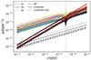 |
Fig. F.1. J1909-3744, sensitivity lines obtained for each parameter, ten random realisations. The vertical line corresponds to the orbital frequency of the binary. The black solid lines correspond to the combination of all parameters. Dashed lines correspond to the case when the linear terms (LTs) are kept |
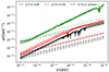 |
Fig. F.3. Five realisations of sensitivity lines using all orbital parameters. Solid lines correspond to cases where all linear terms have been removed, while dashed lines correspond to cases where they have been kept |
We show a few sensitivity lines for two selected pulsars in Figs. F.1 and F.2, and the combined result of all 22 ELL1(H) pulsars in Fig. F.3. Indeed, we can observe that the so-called linear term has a significant effect on the estimated sensitivity derived from δΨ′, both qualitatively (the shape of the curve) and quantitatively (the curve’s normalisation). Fitting only the periodic component gives a less optimistic result and more similar to the results obtained by the two-step approach
The parameters δη and δκ are of particular interest due to the resonance occurring when m = ωb. The depth of the signal relative to the line is approximately determined by the ωbT factor, consistently around three to four orders of magnitude across all studied pulsars. This also suggests that the depth scales with the length of the observation
Large eccentricities
For binary pulsars described by the BT model, the dominant part of the time residual (ignoring the contribution of δK) comes from Eq. (B.1), whereas the variations due to ULDM can be obtained from (C.1) using the definition of αb and ηb in (3) and recalling that ηb ≈ βb. Explicitly,
![$$ \begin{aligned} R^{\mathrm{BT} }&= \, \frac{\delta x}{x}\left[\eta _b \sin E^{\prime }+\alpha _b\left(\cos E^{\prime }-e\right)\right]- \delta e \left[\alpha _b +\frac{e \eta _b\sin E^{\prime }}{1-e^2}+\frac{\sin E^{\prime } \left(\alpha _b \sin E^{\prime }-\eta _b \cos E^{\prime }\right)}{1-e \cos E^{\prime }}\right]\nonumber \\&+\delta \omega x\left[ -\sin E^{\prime } \sin \omega (1-e^2)^{1/2} + \cos \omega \left(\cos E^{\prime }-e\right)\right]-\frac{\delta \Theta ^{\prime } \left(\alpha _b \sin E^{\prime }-\eta _b \cos E^{\prime }\right)}{1-e \cos E^{\prime }} \,, \end{aligned} $$](/articles/aa/full_html/2024/10/aa49953-24/aa49953-24-eq264.gif)
where the variations of δx/x = δa/a, δω, δe, and δΘ′ are given by Eq. (C.1) and, as in the ELL1 case, in this appendix we ignore possible errors in the orbital parameters and secular drifts from other sources, and include the linearly growing term in δΘ′ that depends on the ULDM field
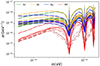 |
Fig. F.4. J1903+0327, five random realisations of sensitivity lines for parameters δx, δe, δω and δΘ′. Dashed lines correspond to the inclusion of linear terms |
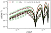 |
Fig. F.5. J1903+0327, five random realisations of sensitivity lines for δΘ′, δΘ′Pb and all combined parameters. Dashed lines correspond to the inclusion of linear terms |
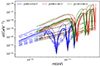 |
Fig. F.6. Five random realisations of sensitivity lines, derived from δΘ′Pb, for J1946+3417, J2234+0611 and J1903+0327. Dashed lines correspond to the inclusion of linear terms |
Five sensitivity curves for δx, δω, δe, δΘ′ are displayed in Fig. F.4. The shape of the sensitivity curves derived from δΘ′ is non-trivial and can vary depending on the value of Υ. The sensitivity obtained from the combination of all parameters, primarily influenced by δΘ′, for all three high-eccentricity pulsars is depicted in Fig. F.5, focusing solely on the first three harmonics. In such figure we also show the sensitivity curves for δΘ′Pb defined in Eq. (65). In agreement to what was shown in Appendix D, the curves for δΘ′Pb only differ from the ones for δΘ′ by order-one factors. The peculiarities related to the linear terms that we mentioned above for δΨ′ are also present for δΘ′ in the BT model and only the ones with no linear terms resemble those found in the two-step method. The combination of all parameters, primarily influenced by δΘ′, for all three high-eccentricity pulsars is depicted in Fig. F.6, focussing solely on the first three harmonics
Sensitivity limit (Gaussian priors)
We aim to compute  in the case of Rayleigh (for 𝜚a) and uniform (for Υa) priors:
In order to compute  , we need to compute the integrals over 𝜚a, Υa and
  . Practically, it is advantageous to first perform the integration over the noise and after that over the variables
  and
and  , leading to two separate Gaussian integrals. For this we decompose RDM into its X and Y components as
where for the ELL1 case we have
![$$ \begin{aligned} Q^{\mathrm{ELL1} }_{X(Y)} = \sin \Psi ^{\prime } A_{X(Y)}^x + x \cos \Psi ^{\prime } \left[A_{X(Y)}^{\Psi ^{\prime }}+L_{X(Y)}^{\Psi ^{\prime }}\right] - x \frac{\cos (2\Psi ^{\prime })+3}{2} A_{X(Y)}^{\eta } + x \frac{\sin (2 \Psi ^{\prime })}{2} A_{X(Y)}^{\kappa } \,, \end{aligned} $$](/articles/aa/full_html/2024/10/aa49953-24/aa49953-24-eq272.gif)
and for the BT model
![$$ \begin{aligned} Q^{\mathrm{BT} }_{X(Y)}&= \,\frac{A_{X(Y)}^a}{a}\left[ \eta _b \sin E^{\prime }+\alpha _b\left(\cos E^{\prime }-e\right)\right]\nonumber \\&- A_{X(Y)}^e \left[\alpha _b +\frac{e \eta _b\sin E^{\prime } }{1-e^2}+\frac{\sin E^{\prime } \left(\alpha _b \sin E^{\prime }-\eta _b \cos E^{\prime }\right)}{1-e \cos E^{\prime }}\right]\nonumber \\&+A_{X(Y)}^\omega x\left[ -\sin E^{\prime } \sin \omega (1-e^2)^{1/2} + \cos \omega \left(\cos E^{\prime }-e\right)\right]\nonumber \\&-\frac{\left[A_{X(Y)}^{\Theta ^{\prime }}+L_{X(Y)}^{\Theta ^{\prime }}\right] \left(\alpha _b \sin E^{\prime }-\eta _b \cos E^{\prime }\right)}{1-e \cos E^{\prime }} \,. \end{aligned} $$](/articles/aa/full_html/2024/10/aa49953-24/aa49953-24-eq273.gif)
After integration over noise and X and Y we obtain
while Σ is defined as
with
where the vector S is defined as

while in the last equation we have ignored the index a, which indicates a particular pulsar. The vectors are indicated by an arrow above the symbols and a dot (⋅) stands for the scalar product
Let us compare the sensitivity limits obtained for both priors (δ-function and Gaussian) when considering a single pulsar
For 𝜚f large (small) the δ-sensitivity limit outperforms (does not outperform) the Gaussian prior. This is an intuitive result, for example when 𝜚f is large, the signal should be strong, so the δ-prior should produce a low-lying sensitivity line, but a Gaussian prior tends to underestimate this signal by leaning more towards the average
We plot sensitivities obtained from both priors for random realisations of 𝜚f (Rayleigh distribution) and Υf (flat distribution). The result is depicted on Fig. F.7. We can notice that most of the δ-sensitivities are above the sensitivities derived from the Gaussian distribution. This result comes out opposite to the one we arrived at in the main body of the paper. We explain this as follows—for a given value of Υf and m, we find the value of 𝜚fEQ so that both sensitivities come out the same
with the function F(m, Υ) given as
For the method described in the main text, the function F would be different, but the numerical factor  is the same. The numerical values may therefore differ slightly, but this is sufficient to change the statistics of the sensitivity lines. For
  , Eq. (F.30) and 30 values of Υ (on the interval [0, 2π) with a constant step), we find that 𝜚fEQ ≥ 1.3. However, this implies P(𝜚 ≥ 1.3)≐0.18. Let us remind that the median of the distribution is
  . Thus, the probability that the sensitivity curve for the δ-prior is lower than that of the Gaussian priors is less than 18%. If the factor F was just slightly smaller, it could lead to a probability larger than 50%. We expect the latter be the case for the method in the main text
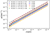 |
Fig. F.7. Sensitivity lines obtained from δ- and Gaussian-priors (Rayleigh-Uniform, or RU) |
All Tables
Three pulsars with notably high eccentricity parametrised by the BT timing model
All Figures
|
Fig. 1. Description of Keplerian orbits in terms of the orbital elements viewed in the fundamental reference frame (X,Y,Z). The Cartesian orbital frame (x,y,z) and the polar one |
| In the text | |
|
Fig. 2. Sensitivity of 22 near-circular binary pulsars, as measured by NANOGrav, to the coupling α as a function of the ULDM mass m. The sensitivities obtained from δx are in black, whereas those pertaining to |
| In the text | |
|
Fig. 3. Same as in Fig. 2 but using 111 binary pulsars from the ATNF catalogue and assuming next-generation radio-telescope precision. We assume Tobs = 10 years, and a next-generation radio-telescope precision given by ϵ = 0.1 μs (based on the analysis presented in Liu et al. (2011) for the upcoming SKA) |
| In the text | |
|
Fig. 4. Sensitivity to α as a function of ULDM mass m for ten realisations of the ULDM parameters 𝜚 and Υ, obtained from the binary pulsar J1946+3417 as measured by NANOGrav |
| In the text | |
|
Fig. 5. Sensitivity to α as a function of ULDM mass m for ten realisations of the ULDM parameters 𝜚 and Υ, obtained from the binary pulsar J2234+0611 as measured by NANOGrav |
| In the text | |
|
Fig. 6. Sensitivity to α as a function of ULDM mass m for ten realisations of the ULDM parameters 𝜚 and Υ, obtained from the binary pulsar J1903+0327 as measured by NANOGrav |
| In the text | |
|
Fig. 7. Sensitivity to α as a function of ULDM mass m for five realisations of the ULDM parameters 𝜚 and Υ, obtained from the combination of the three binary pulsars J1946+3417, J2234+0611 and J1903+0327 as measured by NANOGrav |
| In the text | |
|
Fig. D.1. Sensitivity curves for α as a function of the ULDM mass m for the system J1903+0327 (with parameters given in Table E.2) for masses near the resonant one at ωb = m. Dashed lines account for all the ULDM effects on the parameter Θ′, while the solid lines are obtained neglecting the ULDM effect on all parameters but Pb. Each colour corresponds to a particular random realisation of the parameters 𝜚 and Υ |
| In the text | |
|
Fig. E.1. Sensitivity curves for α as a function of the ULDM mass m for the system J1903+0327 (with parameters given in Table E.2) for masses near the resonant one at ωb = m. Solid lines are obtained after marginalising over all the three nuisance parameters Ξi (i = 0, 1, 2) in the model of Θ′ (we use uniform priors for all of them), dashed lines are obtained after marginalising only over the parameters Ξ0 and Ξ1 (which correspond to a linear growth coefficient and a constant error in Θ′) while the coefficient Ξ2 (which gives a quadratic growth) is assumed to be known and subtracted so that Ξ2 = 0 |
| In the text | |
|
Fig. F.1. J1909-3744, sensitivity lines obtained for each parameter, ten random realisations. The vertical line corresponds to the orbital frequency of the binary. The black solid lines correspond to the combination of all parameters. Dashed lines correspond to the case when the linear terms (LTs) are kept |
| In the text | |
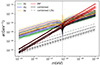 |
Fig. F.2. Same as Fig. F.1 but for the system J2145-0750 |
| In the text | |
|
Fig. F.3. Five realisations of sensitivity lines using all orbital parameters. Solid lines correspond to cases where all linear terms have been removed, while dashed lines correspond to cases where they have been kept |
| In the text | |
|
Fig. F.4. J1903+0327, five random realisations of sensitivity lines for parameters δx, δe, δω and δΘ′. Dashed lines correspond to the inclusion of linear terms |
| In the text | |
|
Fig. F.5. J1903+0327, five random realisations of sensitivity lines for δΘ′, δΘ′Pb and all combined parameters. Dashed lines correspond to the inclusion of linear terms |
| In the text | |
|
Fig. F.6. Five random realisations of sensitivity lines, derived from δΘ′Pb, for J1946+3417, J2234+0611 and J1903+0327. Dashed lines correspond to the inclusion of linear terms |
| In the text | |
|
Fig. F.7. Sensitivity lines obtained from δ- and Gaussian-priors (Rayleigh-Uniform, or RU) |
| In the text | |
Current usage metrics show cumulative count of Article Views (full-text article views including HTML views, PDF and ePub downloads, according to the available data) and Abstracts Views on Vision4Press platform.
Data correspond to usage on the plateform after 2015. The current usage metrics is available 48-96 hours after online publication and is updated daily on week days.
Initial download of the metrics may take a while.