| Issue |
A&A
Volume 683, March 2024
|
|
|---|---|---|
| Article Number | A108 | |
| Number of page(s) | 9 | |
| Section | Stellar atmospheres | |
| DOI | https://doi.org/10.1051/0004-6361/202348778 | |
| Published online | 13 March 2024 | |
Simulating radio-off fractions in rotating radio transients
1
Xinjiang Astronomical Observatory, Chinese Academy of Sciences,
150 Science 1-Street, Urumqi,
Xinjiang
830011, PR China
e-mail: ryuen@xao.ac.cn
2
Xinjiang Key laboratory of Radio Astrophysics, Chinese Academy of Sciences,
150 Science 1-Street, Urumqi,
Xinjiang
830011, PR China
3
Key laboratory of Radio Astronomy, Chinese Academy of Sciences,
Nanjing
210008, PR China
4
SIfA, School of Physics, University of Sydney,
Sydney, NSW
2006, Australia
Received:
29
November
2023
Accepted:
6
January
2024
Aims. We aim to simulate the proportions of non-detectable emission, measured as radio-off fractions (foff), in rotating radio transients (RRATs). We also investigate the properties related to the underlying mechanism for such sporadic emission.
Methods. From observations of intermittent pulsars, radio emission originates from two distinct emission states and it becomes non-detectable when the pulsar switches to an emission state characterized by magnetospheric plasma density of zero. We performed simulations of foff based on 10 000 samples, each with 10 000 rotations and using a model that tracks changes in the plasma density in a pulsar magnetosphere with multiple emission states. We assumed that (i) RRATs are radio pulsars, (ii) radio pulse intensity is correlated with the emitting plasma density as stated in the conventional models, and (iii) a pulse emission corresponds to a change in the plasma density under favorable conditions.
Results. A best-fit distribution for foff is obtained when emission from RRATs is defaulted to radio-off. The resulting wait time distribution can be fitted by two functions of an exponential and a Gaussian, which is consistent with the observations. We demonstrate that the switch rate is low and that the burst rate is dependent on rotation period. In addition, the switch rate is related to the obliquity angle, which implies that the mechanism varies over time. Our results suggest that switching to radio-on is a random process, which implies that the burst rate is different for different RRATs. We show that RRAT emission and pulse nulling may share similar origins, but with different default emission. We discuss how the emission may change from that of RRAT to pulse nulling (or vice versa) as a pulsar evolves.
Key words: radiation mechanisms: non-thermal / pulsars: general
© The Authors 2024
 Open Access article, published by EDP Sciences, under the terms of the Creative Commons Attribution License (https://creativecommons.org/licenses/by/4.0), which permits unrestricted use, distribution, and reproduction in any medium, provided the original work is properly cited.
This article is published in open access under the Subscribe to Open model. Subscribe to A&A to support open access publication.
1 Introduction
There is no consensus on the mechanism for the sporadic bursts of individual pulse from rotating radio transients (RRATs). Discovered in the archival data from Parkes multi-beam pulsar survey (McLaughlin et al. 2006), typical emission from a RRAT exhibits two states: radio-on, when it emits a bright pulse, and radio-off, when it ceases to emit for intervals between tens of seconds to hours, until another pulse is emitted. A common representation for the occurrence of radio-on is expressed in terms of average pulse number per hour (or burst rate, RB1). For the list of RRATs in the RRATalog2, RB is low, which also means that the fraction of radio-off, denoted as foff, is large (cf. Table C.1). Because of this on and off emission, there are suggestions that RRAT emission resembles certain characteristics of pulsar pulse nulling in its extreme form (Wang et al. 2007; Burke-Spolaor & Bailes 2010). This is supported by the measurements of a pulse periodicity, P, in many RRATs (see Appendix C), suggesting that they are rotating neutron stars (Zhang et al. 2007; Burke-Spolaor & Bailes 2010; Keane et al. 2011). This implies that both phenomena are manifested as cessation in the pulsed emission and that their occurrences are random in nature (Ritchings 1976; Biggs 1992). However, alternative models have also been proposed, in which the emission may be results of external interventions (Li 2006; Cordes et al. 2004; Cordes & Shannon 2008).
Some observations of RRATs show that the emission occurs in groups, each of a different time duration (Sun et al. 2021; Zhong et al. 2024). Analyses of the emission from RRAT J1913+1330 reveals that the pulses come in short bursts that last for tens of pulse periods (Zhong et al. 2024). The occurrence of these “burst states” appears random. Furthermore, the pulse emission during the burst states is also random and does not display a correlation with one another. Another example involves the observation of two different emission states from PSR J1752+2359 (Sun et al. 2021). In one state, the pulsar emits ordinary radio pulses, whereas sporadic emission is observed when the pulsar is in the RRAT-like state. Furthermore, both emission states show distinct polarization profiles and polarization position angle swings. This implies that the different emissions may originate from different emission arrangements in the pulsar magnetosphere, each corresponds to a particular emission state. It strongly suggests that RRAT emission arises only under specific emission conditions in an emission state that is “favorable” for such emission. A similar scenario was also observed in some pulsars. For instance, the analysis of nulling from a sample of pulsars revealed that the phenomenon may appear random but the condition that gives rise to the phenomenon may be distinct (Redman & Rankin 2009). In some radio pulsars, pulse nulling has also been shown to display correlation with other emission characteristics (Redman et al. 2005; Rankin & Wright 2007, 2008). However, the occurrence of such favorable conditions is unpredictable and appears random. This suggests that emission from a RRAT requires the existence of a favorable emission condition, which is necessary for the actual emission of a pulse to take place, and both events appear random.
In this paper, we investigate several properties of the underlying emission mechanism for RRATs through simulation of foff. Three facts are relevant. The first information concerns RRATs as radio pulsars (Zhang et al. 2007; Burke-Spolaor & Bailes 2010; Keane et al. 2011). This carries the important implication that the criteria for observable emission from a RRAT is similar to that for a radio pulsar. In particular, emission at a rotational phase, ψ, is related to the viewing, ζ, and obliquity, α, angles measured from the rotation axis to the line of sight and the magnetic axis, respectively. The second and third informations relate to the switching between the two emission states. From observations of intermittent pulsars, their emission also exhibits switching between radio-on and off, but at different timescales (Kramer et al. 2006). Such switching in emission is interpreted as due to changes in the emitting plasma density between two states of abundance and vacuum. This is in agreement with the suggestion that radio pulse intensity is positively correlated with the emitting plasma density (Manchester & Taylor 1977; Cordes 1979; Lyubarskii 1996). We identify the following causes of change in the visible emission in RRATs: (i) RRATs are pulsars; (ii) two different radio emission states exist, each associated with a particular plasma density; (iii) the occurrence of a favorable condition necessary for emission switching; and (iv) switching occurs between two emission states leading to changes in the plasma density and changes between radio-on and off. The points above suggest that the different pulse intensities between radio-on and off in RRATs are due to emission originating from two distinct plasma densities and changes in the emission occur when the plasma density changes. Although a widely accepted model for changes in the plasma density is still lacking, a model has recently been put forward for pulsar magnetospheres of multiple quasi-stable emission states (Melrose & Yuen 2014), between which a pulsar can switch when its emission changes. Furthermore, the unpredictable occurrence of a RRAT emission suggests that the associated emission switching may be a random process.
In Sect. 2, we outline the model for changes in the plasma density in relation to the radio-on and off in RRATs. The simulation procedures and the results are given in Sect. 3. The implications of the results for the properties of the underlying mechanism for RRAT emission is discussed in Sect. 4. We summarize the results in Sect. 5. The necessary informations for the electromagnetic fields and the emission geometry are given in Appendices A and B, respectively, and the samples of RRAT quoted in this paper are listed in Appendix C.
2 Radio-on and off
The notion that RRATs might be pulsar-like (McLaughlin et al. 2006; Burke-Spolaor et al. 2011; Sun et al. 2021) implies that their visibility criteria are similar. In a pulsar magnetosphere of multiple emission states, the plasma charge density for an oblique rotator has the form (Melrose & Yuen 2014):

where the parameter y designates the emission state with values between 0 and 1. The corotation charge density (Goldreich & Julian 1969) is represented by:

where Ecor is the corotation electric field defined by Eq. (A.3). The charge density required to screen the parallel inductive electric field, Eind||, from a rotating magnetic dipole is given by:

where b denotes the unit vector along the dipolar field-lines, and Eind|| is given by Eq. (A.8). For an emission condition corresponding to corotation, we have y = 0 and ρsn = ρGJ. The charge density reduces as y increases reaching a minimal value at ρsn = ρmin for y = 1, where the emission condition is described by the “minimal” model (see Appendix A). For pulsar radio emission, there exists a particle acceleration that leads to the production of electron-positron secondary pairs and screening of the accelerating electric field. The screening takes place if the creation of secondary pairs results in a multiplicity, λ, such that λ = (n+ + n-)/nGJ ≫ 1, where the expression is in the number density for corotation (Gurevich & Istomin 2007; Melrose & Yuen 2012), with nGJ = ρGJ/e and n± being the number density of positrons and electrons. The proportionality of pulse intensity to the plasma density (Cordes 1979; Lyubarskii 1996) means that the former is ∝ λρsn. Assuming identical λ in different emission states means that the pulse intensity is proportional to ρsn. It follows that the radio-off would correspond to ρsn = 0, whereas radio-on is characterized by ρsn ≠ 0. Then, a change in the emission is due to a change in ρsn, which corresponds to a change in the value of y via switching in the emission state. Since ρ = 0 and y = 1 represent two limiting conditions for a pulsar magnetosphere, a radio-off state is considered valid, provided that ρsn = 0 and y = yoff possessing a value between 0 and 1. For a given ψ, there exists only one yoff value for ρsn = 0, and the rest of y = yon values gives ρsn ≠ 0. Therefore, we assume that a yon value always exists for the case where 0 < yon < 1 and yon ≠ yoff for the radio-on state.
Detectable changes in the radio emission requires that the plasma undergoing changes be at the source points visible to the observer. The location of the visible point for a given ψ can be determined by assuming that the radiation from the source point is directed tangentially to the local dipolar magnetic field-lines (Cordes 1978; Hibschman & Arons 2001; Kijak & Gil 2003) and parallel to the line of sight (Gangadhara 2004; Yuen & Melrose 2014). In this geometry, the polar coordinates of the visible point as a function of ψ are specified by Eq. (B.5). The location of the visible point varies resulting in a closed path after one rotation period, referred to as the trajectory of the visible point. In addition, the assumption of emission occurring only within the open-field region suggests that the source points can be specified with a height, rV, given by Eq. (B.8). This way, visible emission is defined by the range of ψ, denoted by Δψ, within which the emission sources locate on the trajectory of the visible point that lies partly or entirely inside the open-field region. A RRAT will demonstrate radio-on and off when the emission region traversed by the trajectory exhibits emission switching between two emission states, with one of them having ρsn = 0 and yoff lying between 0 and 1. The condition of ρsn = 0 may be referred to as a “true” case of radio-off because there actually is no charge density to generate the emission, regardless of the beam structure (Olszanski et al. 2022). This is similarly the case for radio-on with ρsn ≠ 0, despite the pulse intensity.
3 Distribution of foff
To determine foff from an observation, a RRAT should have known P value and the burst rate. We identified 70 RRATs in the RRATalog that meet the requirements. If the emission from a RRAT had been regular, the average pulse number per hour would have been given by RP = 3600 s/P. Hence, the value of foff is

All 70 observed RRATs have high foff values ranging from around 0.8 to near 1, as shown in Fig. 1. Overall, treating RRATs as pulsars means that each RRAT possesses a {ζ, α} pair. Analyses of the polarization position angles from a sample of pulsars (Rankin 1993; Tauris & Manchester 1998) have revealed that the distribution of α lies in the range of ≲90° and becomes highly concentrated toward small values (Rankin 1990). In addition, studues of the radio beam shapes from averaged pulse profiles demonstrates that the relationship between ζ and α is such that the impact parameter β = ζ − α ≲ 10° (Lyne & Manchester 1988). Therefore, we consider α between 1° and 90°, and ζ between 0° and 90°, both in steps of 0.5°, taking into account the impact parameter3 |β| = |t − α| ≤ 15°. Radio emission has been shown to come from a relatively higher height at around 0. 1rL or above (Johnston & Weisberg 2006). Thus, we set the maximum height at 0.2rL for the boundary of the open-field region for every {ζ, α} pair. Then, the pulse window and the associated range of ψ is represented by the part of the trajectory of the visible point that lies inside the open-field region. After that, the eligibility for switching in ρsn for a {ζ, α} pair is determined at each ψ within Δψ by solving Eq. (1) for yoff, such that 0 < yoff ≤ 1 for ρsn = 0. This implies that while yon can possess any values between 0 and 1 (provided that ρsn + 0), yoff is restricted to certain {ζ, α} pairs for a given emission height.
For a RRAT with a particular pair of {ζ, α}, emission requires (i) the presence of a favorable condition for emission switching and (ii) switching of ρsn to occur. We denote the two random processes as p1 and p2, respectively. To search for the best-fit probability for each, the occurrence of each process is calculated based on an interval that is bounded by a fixed minimum value at zero and the maximum value denoted by s1 and s2 for p1 and p2, respectively. Each of the s1 and s2 take a value from the range between 0 and 1, in steps of 0.01. We can consider p1 as an example: an interval is formed for each iteration in s1, such that its maximum value is represented by s1, thus giving an interval of [0, s1]. This gives a total of 101 different intervals. For each iteration in s1, another number is generated randomly from the same range, which is indicated by i1. The condition for emission switching (p1) is considered to have been fulfilled if 0 ≤ i1 ≤ s1 for an iteration in s1. The same is performed for p2 for each iteration in s2, where the random number is indicated by i2. Switching of ρsn will occur provided that 0 ≤ i2 ≤ s2. Therefore, a switching to radio-on requires both 0 ≤ i1 ≤ s1 and 0 ≤ i2 ≤ S2 to be satisfied. We note that the intervals change as s1 and s2 change, hence, the likelihood for meeting the two conditions for an iteration changes accordingly. We further assume that the default emission is radio-off before and after an emission. For given values of ζ and α, the trajectory of the visible point is fixed but the intervals change resulting in the frequency of switching to change in every rotation. We summarize the steps for the simulation in Fig. 2.
When the simulation is completed, each of the 10 000 rotations for a RRAT contains a two-dimensional (2D) array that is 101 by 101. Each of the array elements is filled with either a 0 or 1 from the corresponding values of s1 and s2. Then, the value of foff is calculated from the corresponding elements in each rotation. Here, for the number of rotations, N, the fraction of radio-off is related to the number of times when switching occurs, n, such that foff = 1 − n/N. This gives 101 by 101 values of foff for a RRAT. Distributions of foff are obtained based on values of foff from the corresponding elements in each of the 10 000 rotations from all the 10 000 RRAT samples.
The best-fit distribution for foff from the simulation is shown in Fig. 1. The population is zero for foff ≲ 0.80, above which it shows a near exponential increase reaching a peak at 0.999. The simulation also produces good fits for the peak and the width of the distribution obtained from observations. We found that the average probabilities for p1 and p2 to occur are 0.5 and 0.09, giving a low probability of 0.045 for switching to radio-on. A comparison between the simulated and observed distributions reveals that the former displays more samples for foff between 0.82 and 0.98. We speculate that it is due to the observed samples being too few to represent the whole population of RRATs and so, discovering more RRATs should reduce the discrepancy. For certain RRAT samples in our simulation, the pulses come in groups within tens of periods of each other, whereas the majority of samples show random pulses without distinguishable patterns.
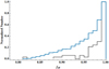 |
Fig. 1 Distributions of foff from 70 observed RRATs (black), and from our simulation (blue). We note that both distributions are normalized to their maximum values. |
4 Properties of the underlying mechanism
In this section, we explore some properties of the mechanism underlying RRAT emission as revealed from our simulation.
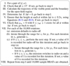 |
Fig. 2 Outline of the simulation procedure. |
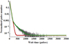 |
Fig. 3 Wait time between two consecutive pulses in our samples. Note: the pulse number is normalized and shown in log scale. The distribution can be fitted using two functions of an exponential and a Gaussian as indicated by the green curve, whereas the curve in red represents the exponential function only. |
4.1 Wait times
A useful means for describing the bursts (radio-on) is the waiting time period in which a RRAT is detected with the next emission. The distribution of such wait times from our samples is shown in Fig. 3. It demonstrates that most pulses come within relatively short periods of each other, together with an extended tail of long wait times and a secondary distribution at around the middle. There are about 50% of the bursts occur at a wait time of less than ten pulses and about 80% with a wait time of less than 30 pulses. For our samples, the wait time can be fitted using two functions of an exponential and a Gaussian. The exponential function fits for the pulses with short wait times and at the long tail, and the Gaussian is required to fit the second distribution in-between. The use of two different functions for fitting is consistent with that observed in several RRATs (Karako-Argaman et al. 2015; Shapiro-Albert et al. 2018). From the analysis of wait times in three RRATs based on long datasets, Shapiro-Albert et al. (2018) showed that each of the wait time distributions also requires fitting with an exponential and a Gaussian. In our samples, the trend for an increase in bursts at short wait times and the overall decrease in the burst number as the wait time increases, is also consistent with observations (Shapiro-Albert et al. 2018; Xie et al. 2022b). It is apparent that the parameters for fitting the curves of different foff distributions are different, which in turn is dependent on the switch rate.
It is apparent that the mechanism underlying RRAT emission is related to the wait time, which, in turn, is dependent on the switch rate. The switch rate, or the occurrence rate, is given by 0.045 for 10000 rotations. It is then possible to estimate the burst rate (RB) for a RRAT with known P using the switch rate obtained from our simulation. Figure 4 shows the curve for RB as a function P over the range of RB defined by the 70 observed RRATs in Table C.1. The burst rate is low at large P and increases roughly exponentially as P decreases. A similar trend has also been observed from the 70 RRATs, where an increasing number of RRATs with larger RB, is seen as P decreases. Our simulation suggests that the mechanism for switching to radio-on resembles a random process of low occurrence probability. For regular emission, like that of a pulsar, the wait time is identical for any two consecutive pulses. The existence of different wait times in a RRAT may be an indication of the emission coming from different evolutionary stages of a pulsar (cf. Sect. 4.2).
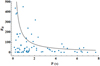 |
Fig. 4 Burst rate (h−1) as a function of P for the 70 observed RRATs (blue points) and that predicted from our simulation (gray curve). |
4.2 Emission evolution
Assuming RRATs as pulsars leads to the question of how important the obliquity angle is to the sporadic emission and its relationship. In our simulation, a burst from a RRAT corresponds to switching in the charge density to non-zero and more bursts (higher burst rate) correspond to more such switching. The variation in the number of switching as a function of α is shown in Fig. 5. More switching is found at small α followed by a rapid decrease by nearly 80% at α ~ 10°. The distribution continues to drop as α increases and becomes roughly constant over 30° ≲ α ≲ 75°. Then, it begins to decrease again reaching zero at α = 90°. In addition, 50% of the samples possess α ≤ 12°, and increases to 80% for α ≤ 48°. This indicates that emission switching, in relation to RRAT emission, is more frequent at small α than that at large α, meaning that frequent RRAT emission favors small α.
The variation in the number of switching as α changes also implies that the underlying mechanism for RRATs evolves over time. For radio pulsars, there are broadly two models for the evolution of α. One model relates the energy loss to the mag-netodipole radiation. The value of α evolves from large to small, where braking is also from large to small, till its reaches α = 0° when there is no electromagnetic radiation (Manchester & Taylor 1977; Lyubarskii & Kirk 2001). The other model considers the energy loss as due to the longitudinal current flow and the production of secondary particles in the magnetosphere (Beskin et al. 1988). This implies the evolution of α from small to large, where the spin-down rate obtains its maximal in the axisymmetric case and decreases as the plasma decreases with α approaching 90° (Goldreich & Julian 1969). Furthermore, pulsar radio emission is suggested originating from pair production under an accelerating potential which decreases as the pulsar rotation period increases. The pair production, and hence the radio emission, would stop once the accelerating potential falls below certain threshold value. Based on the ATNF Pulsar Catalogue4 (Manchester et al. 2005), we see that ordinary pulsars possess an average rotation period of about 1 s. The mean rotation period averaged from the 70 RRATs in Table C.1 is 2.14 s, and the percentage for P > 1 s is about 64.1%. This indicates that the rotation period of RRATs tends to be higher than ordinary pulsars (Karako-Argaman et al. 2015). More RRATs having larger P signifies that they represent later stages in pulsar evolution. From Fig. 4, a RRAT with longer rotation period is likely to have a lower RB, or lower switching, which corresponds to larger α in Fig. 5. This is in favor of the second model for energy loss, in which α evolves from small to large. This also implies that their sparse emission may be due to the accelerating potential dropping near the threshold (Zhang et al. 2007) resulting in a “production shortage” of pairs. It may be that the existence of a wait time is for accumulating sufficient plasma pairs for the next emission. It is obvious that the length of the wait time and the amount of pairs to accumulate are dependent on the RRAT. Considering switching to radio-on is a random process would imply that the ending of an accumulation period is also random. It follows that the plasma pairs may be overaccumulated in some RRATs. When such a RRAT eventually emits, the emission may be exhibited as continuous pulsed emission, such as that observed in PSR J1752+2359 (Sun et al. 2021) and PSR J1839−0141 (Cui et al. 2017).
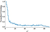 |
Fig. 5 Variation of the normalized number of switching as a function of α. |
4.3 Nulling and RRATs
Other properties of the mechanism underlying RRATs are revealed when comparing with another phenomenon known as pulse nulling. The latter also exhibits as cessation of the single pulses, but at a much shorter timescales. There were suggestions that RRATs and nulling may be two different manifestations of the same mechanism (Burke-Spolaor & Bailes 2010). The major difference between the two phenomena lies in the foff. When applied to nulling, the foff receives a more popular name called the nulling fraction, or NF. The NFs in most nulling pulsars are found with small values such that the distribution of the NFs displays a single prominent peak located around low values, and then decreases roughly exponentially as the NF increases (Wang et al. 2020). There are two obvious differences between the distributions of NF and foff. First, the distribution of foff for RRATs peaks at foff ≈ 1, whereas distribution of NFs peaks at near zero. Second, the values of NF can exists virtually anywhere between 0 and 1, with a different population, while foff is concentrated in a small region near foff ≈ 1. It is straightforward to produce a distribution that peaks near zero using the exact same procedures outlined in Sect. 3 with a single modification to the default emission state. For nulling, the default emission state is radio-on. The resulting NF distribution is almost a mirror image of the foff distribution, such that the distribution is narrow and concentrates over a range near zero. A simulation for the full distribution of NF would require extra assumptions and emission conditions in addition to that made for RRATs. This indicates that the origin of nulling and RRAT emission may share some similarities. How-ever, it also highlights a significant difference between RRAT emission and nulling, namely, that RRATs do not exhibit a tendency toward emitting, whereas nulling pulsars do exhibit that tendency.
5 Summary and discussion
We summarize the properties of the underlying mechanism for RRATs as revealed by our results below.
The default emission is radio-off.
An emission change is required to turn to radio-on.
Switching to radio-on is a random process of a low-probability occurrence.
The burst rate changes over time, with higher burst rates favoring small P and small α.
RRAT and nulling may share similar origins.
The assumed default emission and treating RRATs as pulsars have an observational implication. The suggestion that α and, hence, β changes as a pulsar evolves implies that the locus where the trajectory of the visible point cuts the open-field region will change over time (see Eqs. (B.5) and (B.8)). From Eq. (1), this also implies a change in ρsn = 0 along the trajectory causing the observed emission to vary with time. In addition, some studies of pulsars reveal different emission properties at different parts of an integrated profile (Rankin & Wright 2008; Gajjar et al. 2017; Tu et al. 2022), showing that the emission condition across the emission region is not likely to be uniform. The default emission, as we assumed for the RRAT samples, is apparently related to the emission conditions in the emission region. This means that the observed default emission may depend on where the trajectory cuts the emission region. For example, a change in default emission between radio-on and off will result in the observable emission to change between pulse nulling and that from RRATs as the pulsar evolves. Such changes would require regular observations of RRATs and nulling pulsars, as well as an accurate measurement of their ζ and α angles. A common method for estimating the two parameters is through the modeling of the changes in the polarization position angle across the profile window (Lyne & Manchester 1988). The result is sensitive to the quality of the data. In addition, a correct differentiation of a null from a very weak emission requires a highly sensitive and powerful telescope. This is realized with the observing power of FAST (Li et al. 2018) and the availability of future telescopes and large arrays, such as the 110-m QiTai radio Telescope (QTT) and the Square Kilometer Array (SKA). With the discovering power of more than 2000 new pulsars in 43 days (Xie et al. 2022a), the QTT (Wang 2014) stands as a promising tool for delivering higher quality observational data for investigations of pulsar emission mechanism.
Acknowledgements
We thank the XAO pulsar group for useful discussions. We also thank the anonymous referee for constructive suggestions that improved the presentation of this manuscript. R.Y. is supported by the National SKA Program of China No. 2020SKA0120200, the National Key Program for Science and Technology Research and Development No. 2022YFC2205201, the National Natural Science Foundation of China (NSFC) project (Nos. 12288102,12041303, 12041304), the Major Science and Technology Program of Xinjiang Uygur Autonomous Region No. 2022A03013-2, and the open program of the Key Laboratory of Xinjiang Uygur Autonomous Region No. 2020D04049. This research is partly supported by the Operation, Maintenance and Upgrading Fund for Astronomical Telescopes and Facility Instruments, budgeted from the Ministry of Finance of China (MOF) and administrated by the CAS.
Appendix A The magnetic and electric fields
In the model for obliquely rotating pulsar magnetopsheres of multiple emission states, the electric field may be written as (Melrose & Yuen 2014):

The Epot term represents the electric field in association with the corotation charge density, namely, Epot = −grad Φcor. The term Eind is the inductive electric field produced by the obliquely rotating magnetic dipole in the form defined by:
![${{\bf{E}}_{{\rm{ind}}}} = {{{\mu _0}} \over {4\pi }}\left[ {{{{\bf{x}} \times {\bf{\dot \mu }}} \over {{r^3}}} + {{{\bf{x}} \times {\bf{\ddot \mu }}} \over {{r^2}c}}} \right].$](/articles/aa/full_html/2024/03/aa48778-23/aa48778-23-eq6.png)
In the above equations, the position vector and radial distance from the stellar center are indicated by x and r, respectively, and the time-dependent magnetic dipole is given by µ. In addition, the light speed is given by c and µ0 is the vacuum permeability. The parameter y represents an emission state with a value between 0 and 1. An emission state that signified by y = 0 corresponds to the corotation model (Goldreich & Julian 1969), where E = Ecor is the corotation electric field with Ecor. Assuming a plasma-filled magnetosphere with infinite conductivity and negligible particle inertia, the electric field vanishes in the co-moving frame of the plasma giving:

where ω⋆ is the angular velocity of the star, and the magnetic field for a rotating magnetic dipole in vacuo are of the form given by (Melrose & Yuen 2014):
![${\bf{B}} = {{{\mu _0}} \over {4\pi }}\left[ {{{3{\bf{xx}} \cdot {\bf{\mu }} - {r^2}{\bf{\mu }}} \over {{r^5}}} + {{3{\bf{xx}} \cdot {\bf{\dot \mu }} - {r^2}{\bf{\dot \mu }}} \over {{r^4}c}} + {{{\bf{x}} \times \left( {{\bf{x}} \times {\bf{\ddot \mu }}} \right)} \over {{r^3}{c^2}}}} \right].$](/articles/aa/full_html/2024/03/aa48778-23/aa48778-23-eq8.png)
Here, the term ∝ 1/r3 is the dipolar term, and the radiative term is denoted by the two terms proportional to 1/r2 and ∝ 1/r. For obliquely rotating magnetospheres, Equation (A.3) can be expressed through the form (Hones & Bergeson 1965; Melrose 1967):

where the vector potential due to a rotating magnetic dipole is represented by V (Melrose & Yuen 2014), and Eind = −∂V/∂t. Expressed in spherical coordinates, the Ecor has components along only the radial and polar directions, and perpendicular to the field-lines, in a dipolar field structure.
An emission state designated by y = 1 corresponds to the “minimal” model (Melrose & Yuen 2014), in which the parallel electric field, Eind||, is screened and the perpendicular component, Eind⊥, possesses the same value as that in the vacuum-dipole model, which takes the form given by Equation (A.2). Adding the divergence gives (Melrose & Yuen 2012):

where the distance along dipolar magnetic field-lines is signified by s, and Eind|| = Eind · b. The b represents the unit vector along dipolar magnetic field-lines; when considering the curvature of the field-lines, it takes the following form (Melrose & Yuen 2012):

in spherical polar coordinates relative to the rotation axis. The  denote the unit vectors in radial, polar, and azimuthal directions, respectively, and Θ = (3 cos2 θm + 1)1/2, where θm = cos α cos θ + sin α sin θ cos(ϕ − ψ). Designating the time-dependent magnetic dipole as µ, we then have:
![${E_{\left. {{\rm{ind}}} \right\|}} = {{{\mu _0}} \over {4\pi }}{{{\bf{b}} \cdot \left[ {{\bf{x}} \times \left( {{{\bf{\omega }}_*} \times {\bf{\mu }}} \right)} \right]} \over {{r^3}}}.$](/articles/aa/full_html/2024/03/aa48778-23/aa48778-23-eq13.png)
All the above equations are valid for an oblique rotator (α ≠ 0). For the location of a given set of coordinates, unique values for both B and E can be determined for known ζ and α (see Appendix B).
Appendix B Geometry for observable emission
The rotation and magnetic axes of a pulsar are arranged in Cartesian coordinates such that  and
and  , respectively, with unit vectors given by
  , ŷ, ẑ and
  , ŷb, ẑb. The transformation between the unit vectors is given by:

where

and RT is the transpose of R. The corresponding unit vectors for radial, polar and azimuthal in spherical coordinates are represented by  and
and  , and
, and

with

indicating the transformation.
We assume an idealized model for pulsar visibility where pulsar emission occurs at the source point that is located only within the open-field region (Cordes 1978; Kijak & Gil 2003). The emission is directed along the local magnetic field line of dipolar structure (Hibschman & Arons 2001) and parallel to the line-of-sight direction (Yuen & Melrose 2014). We neglect the aberration effect and the size of the forward cone in pulsar radio radiation due to relativistic plasma streaming along curved magnetic field lines. In this model. pulsar emission from highly relativistic particles is strongly confined to a narrow forward cone. A dipolar field line, which diminishes proportionally according to 1/r3, is defined by two constants: r0 = r/ sin2 θb and Φ0 = ϕb, where Φ0 is the azimuthal position of the field line at the stellar surface. The location of the visible point is designated by (θV, ϕV) or (θbV, ϕbV), at a particular ψ for known ζ and α. It is given by (Gangadhara 2004; Yuen & Melrose 2014):

where cos Γ = cos a cos ζ + sin a sin ζ cos(ϕ − ψ) is the half-opening angle of the emission beam. The conversions from (θb, ϕb) to (θ, ϕ) are given by:


The solutions relevant to our discussion correspond to the path traced by the visible point, referred to as the trajectory of the visible point, from the nearer of the two magnetic poles relative to ψ = 0. Here, the impact parameter, β = ζ − α, is at a minimum. Pulsar radio radiation from relativistic plasma streaming along curved magnetic field lines leads to the emission being confined into a narrow forward cone that is directed about the tangent, but aberrated at a small angle to the field line (Melrose 1995; Lyutikov et al. 1999). Equation (B.5) implies the neglect of the size of this cone and the related effects.
The assumption that emission occurs only within the open-field region (or “polar-cap region”) introduces the dependence of height, such that the boundary of this region is defined by the locus of the last closed field lines, which satisfy θb = arcsin  and 0 ≤ ϕb < 2π, with r0 = rL; also, rL = c/ω⋆ is the light-cylinder radius. This implies that the boundary is dependent on both ψ and r. Emission can be seen from the height, r, only when the trajectory of the visible point is inside this boundary and the edges of the pulse window are defined by the rotational phases when the trajectory crosses this boundary. The pulse window is reduced to one point (if only one pole is visible) at a particular ψ and from a height, r = rmin, where the trajectory is tangential to the boundary in a more restrictive context. This indicates that the emission is present only along the last closed field line. This implies the dependence of the visible point on height, denoted by rV, in the form of the following requirement for each open-field line: rV > rmin. The rV at a particular ψ is given by:

Here θbL represents the polar angle of the point on the last closed field line.
Appendix C The RRATs
We list the parameters of the RRATs related to the analysis in this paper below. The values for foff are obtained using Equation (4).
Details of the RRATs obtained from The RRATalog website are shown in the first three columns.
References
- Beskin, V., Gurevich, A. V., & Istomin, Y. N. 1988, Astrophys. Space Sci., 146, 205 [NASA ADS] [CrossRef] [Google Scholar]
- Biggs, J. D. 1992, ApJ, 394, 574 [NASA ADS] [CrossRef] [Google Scholar]
- Burke-Spolaor, S., & Bailes, M. 2010, MNRAS, 402, 855 [Google Scholar]
- Burke-Spolaor, S., Bailes, M., Johnston, S., et al. 2011, MNRAS, 416, 2465 [NASA ADS] [CrossRef] [Google Scholar]
- Cordes, J. M. 1978, ApJ, 222, 1006 [NASA ADS] [CrossRef] [Google Scholar]
- Cordes, J. M. 1979, Space Sci. Rev., 24, 567 [NASA ADS] [CrossRef] [Google Scholar]
- Cordes, J. M., & Shannon, R. M. 2008, ApJ, 682, 1152 [NASA ADS] [CrossRef] [Google Scholar]
- Cordes, J. M., Bhat, N. D. R., Hankins, T. H., McLaughlin, M. A., & Kern, J. 2004, ApJ, 612, 375 [NASA ADS] [CrossRef] [Google Scholar]
- Cui, B.-Y., Boyles, J., McLaughlin, M. A., & Palliyaguru, N. 2017, ApJ, 840, 5 [NASA ADS] [CrossRef] [Google Scholar]
- Gajjar, V., Yuan, J. P., Yuen, R., et al. 2017, ApJ, 850, 173 [NASA ADS] [CrossRef] [Google Scholar]
- Gangadhara, R. T. 2004, ApJ, 609, 335 [NASA ADS] [CrossRef] [Google Scholar]
- Goldreich, P., & Julian, W. H. 1969, ApJ, 157, 869 [Google Scholar]
- Gurevich, A. V., & Istomin, Y. N. 2007, MNRAS, 377, 1663 [NASA ADS] [CrossRef] [Google Scholar]
- Hibschman, J., & Arons, J. 2001, ApJ, 554, 624 [NASA ADS] [CrossRef] [Google Scholar]
- Hones, E. W. J., & Bergeson, J. E. 1965, JGR, 70, 4951 [NASA ADS] [CrossRef] [Google Scholar]
- Johnston, S., & Weisberg, J. M. 2006, MNRAS, 368, 1856 [NASA ADS] [CrossRef] [Google Scholar]
- Karako-Argaman, C., Kaspi, V. M., Lynch, R. S., et al. 2015, ApJ, 809, 67 [NASA ADS] [CrossRef] [Google Scholar]
- Keane, E. F., Kramer, M., Lyne, A. G., Stappers, B. W., & McLaughlin, M. A. 2011, MNRAS, 415, 3065 [Google Scholar]
- Kijak, J., & Gil, J. 2003, A&A, 397, 969 [NASA ADS] [CrossRef] [EDP Sciences] [Google Scholar]
- Kramer, M., Lyne, A. G., O’Brien, J. T., Jordan, C. A., & Lorimer, D. R. 2006, Science, 312, 549 [NASA ADS] [CrossRef] [Google Scholar]
- Li, D., Wang, P., Qian, L., et al. 2018, IEEE Microwave, 19, 112 [NASA ADS] [CrossRef] [Google Scholar]
- Li, X. D. 2006, ApJ, 646, L139 [NASA ADS] [CrossRef] [Google Scholar]
- Lyne, A. G., & Manchester, R. N. 1988, MNRAS, 234, 477 [NASA ADS] [CrossRef] [Google Scholar]
- Lyubarskii, Y. E. 1996, A&A, 308, 809 [NASA ADS] [Google Scholar]
- Lyubarskii, Y. E., & Kirk, J. G. 2001, ApJ, 547, 437 [NASA ADS] [CrossRef] [Google Scholar]
- Lyutikov, M., Blandford, R. D., & Machabeli, G. 1999, MNRAS, 305, 338 [NASA ADS] [CrossRef] [Google Scholar]
- Manchester, R. N., & Taylor, J. H. 1977, Pulsars (San Francisco: W. H. Freeman) [Google Scholar]
- Manchester, R. N., Hobbs, G. B., Teoh, A., & Hobbs, M. 2005, AJ, 129, 1993 [Google Scholar]
- McLaughlin, M. A., Lyne, A. G., Lorimer, D. R., et al. 2006, Nature, 439, 817 [NASA ADS] [CrossRef] [Google Scholar]
- Melrose, D. B. 1967, Planet. Space. Sci., 15, 381 [NASA ADS] [CrossRef] [Google Scholar]
- Melrose, D. B. 1995, J. Astrophys. Astr., 16, 137 [NASA ADS] [CrossRef] [Google Scholar]
- Melrose, D. B., & Yuen, R. 2012, ApJ, 745, 169 [NASA ADS] [CrossRef] [Google Scholar]
- Melrose, D. B., & Yuen, R. 2014, MNRAS, 437, 262 [NASA ADS] [CrossRef] [Google Scholar]
- Olszanski, T., Rankin, J., Venkataraman, A., & Wahl, H. 2022, MNRAS, 517, 1189 [NASA ADS] [CrossRef] [Google Scholar]
- Rankin, J. M. 1990, ApJ, 352, 247 [Google Scholar]
- Rankin, J. M. 1993, ApJS, 85, 145 [NASA ADS] [CrossRef] [Google Scholar]
- Rankin, J. M., & Wright, G. A. E. 2007, MNRAS, 379, 507 [NASA ADS] [CrossRef] [Google Scholar]
- Rankin, J. M., & Wright, G. A. E. 2008, MNRAS, 385, 1923 [NASA ADS] [CrossRef] [Google Scholar]
- Redman, S. L., & Rankin, J. M. 2009, MNRAS, 395, 1529 [NASA ADS] [CrossRef] [Google Scholar]
- Redman, S. L., Wright, G. A. E., & Rankin, J. M. 2005, MNRAS, 357, 859 [NASA ADS] [CrossRef] [Google Scholar]
- Ritchings, R. T. 1976, MNRAS, 176, 249 [NASA ADS] [Google Scholar]
- Shapiro-Albert, B. J., McLaughlin, M. A., & Keane, E. F. 2018, ApJ, 866, 152 [NASA ADS] [CrossRef] [Google Scholar]
- Sun, S. N., Yan, W. M., Wang, N., & Yuen, R. 2021, RAA, 21, 240 [NASA ADS] [Google Scholar]
- Tauris, T. M., & Manchester, R. N. 1998, MNRAS, 298, 625 [NASA ADS] [CrossRef] [Google Scholar]
- Tu, Z. Y., Yuen, R., Wen, Z. G., et al. 2022, MNRAS, 512, 1906 [NASA ADS] [CrossRef] [Google Scholar]
- Wang, N. 2014, SSPMA, 44, 783 [NASA ADS] [CrossRef] [Google Scholar]
- Wang, N., Manchester, R. N., & Johnston, S. 2007, MNRAS, 377, 1383 [Google Scholar]
- Wang, P. F., Han, J. L., Han, L., et al. 2020, A&A, 644, A73 [NASA ADS] [CrossRef] [EDP Sciences] [Google Scholar]
- Wang, P. F., Han, J. L., Xu, J., et al. 2023, RAA, 23, A02 [Google Scholar]
- Xie, J. T., Wang, J. B., Wang, N., & Hu, Y. 2022a, Res. Astron. Astrophys., 22, 075009 [CrossRef] [Google Scholar]
- Xie, J. T., Wang, J. B., Wang, N., et al. 2022b, ApJ, 940, L21 [NASA ADS] [CrossRef] [Google Scholar]
- Yuen, R., & Melrose, D. B. 2014, PASA, 31, e039 [NASA ADS] [CrossRef] [Google Scholar]
- Zhang, B., Gil, J., & Dyks, J. 2007, MNRAS, 374, 1103 [Google Scholar]
- Zhong, W. Q., Zhi, Q., Lu, J., et al. 2024, MNRAS, 527, 4129 [Google Scholar]
Recent studies have shown a larger sample of β and α values (Wang et al. 2023). The position angle curve in some of these pulsars follow an S-shape curve, and their radio emission is found to originate at finite heights. This is consistent with the assumption that pulsar radio emission comes from inner magnetosphere of a dipolar field structure. A dipolar field-line structure is symmetric between the northern and southern magnetic hemispheres, apart from a phase different of π, hence, our calculation remains valid.
All Tables
Details of the RRATs obtained from The RRATalog website are shown in the first three columns.
All Figures
|
Fig. 1 Distributions of foff from 70 observed RRATs (black), and from our simulation (blue). We note that both distributions are normalized to their maximum values. |
| In the text | |
|
Fig. 2 Outline of the simulation procedure. |
| In the text | |
|
Fig. 3 Wait time between two consecutive pulses in our samples. Note: the pulse number is normalized and shown in log scale. The distribution can be fitted using two functions of an exponential and a Gaussian as indicated by the green curve, whereas the curve in red represents the exponential function only. |
| In the text | |
|
Fig. 4 Burst rate (h−1) as a function of P for the 70 observed RRATs (blue points) and that predicted from our simulation (gray curve). |
| In the text | |
|
Fig. 5 Variation of the normalized number of switching as a function of α. |
| In the text | |
Current usage metrics show cumulative count of Article Views (full-text article views including HTML views, PDF and ePub downloads, according to the available data) and Abstracts Views on Vision4Press platform.
Data correspond to usage on the plateform after 2015. The current usage metrics is available 48-96 hours after online publication and is updated daily on week days.
Initial download of the metrics may take a while.