| Issue |
A&A
Volume 689, September 2024
|
|
|---|---|---|
| Article Number | A165 | |
| Number of page(s) | 12 | |
| Section | Cosmology (including clusters of galaxies) | |
| DOI | https://doi.org/10.1051/0004-6361/202348542 | |
| Published online | 12 September 2024 | |
Standardizing the gamma-ray burst as a standard candle and applying it to cosmological probes: Constraints on the two-component dark energy model
1
School of Physics and Physical Engineering, Qufu Normal University, Qufu 273165, China
2
School of Astronomy and Space Science, Nanjing University, Nanjing 210023, China
3
Key Laboratory of Modern Astronomy and Astrophysics (Nanjing University) Ministry of Education, China
Received:
10
November
2023
Accepted:
27
May
2024
Abstract
As one of the most energetic and brightest events, gamma-ray bursts (GRBs) have been used as a standard candle for cosmological probes. Based on the relevant features of the GRB light curve, namely a plateau phase followed a decay phase, we obtain X-ray samples of 31 GRBs and optical samples of 50 GRBs, which are thought to be caused by the same physical mechanism. We standardize GRBs using the two-dimension fundamental plane relation of the rest-frame luminosity of the plateau emission (Lb, z) and the end time of plateau (Tb, z) Lb, z − Tb, z, as well as the three-dimensional fundamental plane correlation including the peak energy (Ep, i) Lb, z − Tb, z − Ep, i. For the cosmological probes, we consider the ωCDM model in which the dark energy consists of one component, and mainly focus on the X1X2CDM model in which the dark energy is made up of two independent components. We obtain constraints on the related parameters of the cosmological models using type Ia supernovae (SNe Ia) data and selected X-ray and optical samples. For the X1X2CDM model, we find that the values of the equation-of-state parameters of two dark energies, ω1 and ω2, are very close. We also carry out a comparison between the models using the Bayesian information criterion, and find that the ωCDM model is favored.
Key words: gamma-ray burst: general / dark energy
Corresponding authors; This email address is being protected from spambots. You need JavaScript enabled to view it. , This email address is being protected from spambots. You need JavaScript enabled to view it. , This email address is being protected from spambots. You need JavaScript enabled to view it. .
© The Authors 2024
 Open Access article, published by EDP Sciences, under the terms of the Creative Commons Attribution License (https://creativecommons.org/licenses/by/4.0), which permits unrestricted use, distribution, and reproduction in any medium, provided the original work is properly cited.
This article is published in open access under the Subscribe to Open model. This email address is being protected from spambots. You need JavaScript enabled to view it. to support open access publication.
1. Introduction
Studies of Type Ia supernovae (SNe Ia) have revealed the accelerating expansion of the Universe (Riess et al. 1998; Perlmutter et al. 1999), which has been confirmed by several independent cosmological probes, such as the cosmic microwave background (CMB; Spergel et al. 2003; Planck Collaboration XVI 2014; Planck Collaboration XIII 2016; Planck Collaboration VI 2020) and baryon acoustic oscillation (BAO; Eisenstein et al. 2005). It has been hypothesized that an unknown component of the Universe – contributing significantly to the current cosmic energy budget – named dark energy (DE) (Copeland et al. 2006; Frieman et al. 2008; Durrer & Maartens 2008) causes this acceleration of the Universe. Most cosmological observations agree well with the flat Λ cold dark matter (CDM) model. However, other alternative DE models, such as ωCDM, ϕCDM, and so on (Peebles & Ratra 1988; Ratra & Peebles 1988; Pavlov et al. 2013; Ong 2023), have not been ruled out given the precision of current measurements. Many DE models contain only a single component with an equation-of-state parameter ω = p/ρ. Gong & Chen (2007) proposed a different DE model (X1X2CDM model) with two components, ω1 and ω2, and they used data for gamma-ray bursts (GRBs) and SNe Ia to investigate the proposed DE model. Here, we consider the two components of the DE model and investigate the constraints on the related cosmological parameters.
Many cosmological probes, such as SNe Ia, CMB, and so on, have been employed for testing cosmological models. The maximum observable redshift of SNe Ia is currently about z ∼ 2.3 (Scolnic et al. 2018), and the CMB provides meaningful information to about z ∼ 1100. Obviously, there is a redshift gap between SNe Ia and the CMB. It has been proposed that GRBs are very promising as a complement to SNe Ia and the CMB, providing us with the opportunity to explore the blank history of the Universe.
GRBs are the most violent bursts in the Universe, with very high energy and brightness that occur in a very short period of time (Klebesadel et al. 1973; Mészáros 2006; Gehrels et al. 2009; Wang & Dai 2011; Kumar & Zhang 2015). They can be split into long (LGRBs, T90 > 2s) or short bursts (SGRBs, T90 < 2s) based on the bimodal duration time T90 (Kouveliotou et al. 1993; Qin et al. 2013). The maximum observed redshift of GRBs is about z ∼ 9.4 (Cucchiara et al. 2011), and could theoretically reach z ∼ 20 (Lamb & Reichart 2000). Furthermore, unlike SNe Ia, gamma-ray photons are mostly unaffected by the interstellar medium (ISM) as they travel towards us (Wang et al. 2015). Given these advantages, GRBs become a particularly appealing cosmological probe and can be employed to investigate the characteristics of the Universe at high redshift; indeed they are expected to provide effective constraints on the parameters of cosmological models (Dai et al. 2004; Ghirlanda et al. 2004a; Liang & Zhang 2006; Schaefer 2007; Kodama et al. 2008; Wang et al. 2011; Amati & Della Valle 2013; Wei & Wu 2017; Wei et al. 2018; Khadka et al. 2021; Dainotti et al. 2022a,b).
Compared with SNe Ia, the luminosity of GRBs covers several orders of magnitude and cannot be directly applied to the cosmological probe as a “standard candle”. Many correlations (e.g., Amati et al. 2002; Ghirlanda et al. 2004b; Yonetoku et al. 2004; Dainotti et al. 2008; Liang & Zhang 2005; Zhao et al. 2020) have been proposed for the related parameters of the prompt and afterglow emission of GRBs. Based on these correlations, GRBs can be standardized as a standard candle for the purposes of the cosmological probes (Cao et al. 2022a,b,c; Jia et al. 2022; Liang et al. 2022; Liu et al. 2022; Li et al. 2023a). Many attempts have been made to treat GRBs as a standard candle, using the correlations to constrain the cosmological parameters (Cardone et al. 2009; Postnikov et al. 2014; Amati et al. 2019; Tang et al. 2019; Cao et al. 2021; Dainotti et al. 2021, 2022a, 2023; Xu et al. 2021; Jia et al. 2022; Tian et al. 2023). In this paper, we investigate the two-parameter correlation between the luminosity (Lb, z) and the end time of the plateau (Tb, z) Lb, z − Tb, z, and the three-parameter correlation including the peak energy (Ep, i) Lb, z − Tb, z − Ep, i.
With the increased number of GRBs, a subclass of GRBs with a plateau phase has been discovered. According to Swift observations, some GRBs exhibit an X-ray afterglow plateau phase followed by a normal decay phase (Zhang et al. 2006; Nousek et al. 2006; O’Brien et al. 2006; Liang et al. 2007; Yi et al. 2015, 2016, 2021; Li et al. 2023b). Specifically, if the central engine is powered by the rotational energy of a newborn, strongly magnetic neutron star, the injection of energy could result in a plateau phase (Dai & Lu 1998b; Zhang & Mészáros 2001; Metzger et al. 2011). The release of energy from the central engine leads to spin down of the magnetar. The energy released by different radiation processes will lead to different changes to the decay index in the decay stage of the light curve. For instance, if gravitational wave (GW) emission or magnetic dipole (MD) radiation predominate, the decay index of the X-ray light curve will be −1 or −2, respectively (Dai & Lu 1998b; Zhang & Mészáros 2001). GRBs chosen from the same physical origin are considered to be suitable for cosmological purposes. In previous work, we selected a class of GRBs with this characteristic and looked into the potential correlations Lb, z − Tb, z − Eγ, iso and Lb, z − Tb, z − Ep, i (Si et al. 2018; Li et al. 2023c), where we used the selected X-ray sample (31 GRBs from Wang et al. 2022) and an optical sample (50 GRBs from Si et al. 2018). More detailed information can be found in Sects. 3 and 4.
When employing the model-dependent GRB data, the circularity problem is inevitable (Ghirlanda et al. 2006) when constraining the cosmological parameters, and many works have aimed to solve this problem (Amati et al. 2008, 2019; Liang et al. 2008; Jimenez & Loeb 2002; Jimenez et al. 2003). Following previous work, here we calibrate the correlation by combining the Hubble parameter data and the Gaussian process (GP) method. This procedure is explained in detail in Sect. 4.2. In this paper, the two selected samples (X-ray and optical samples) are used and combined with a sample of SNe Ia to give limiting results for the free parameters of the two-component DE model and the one-component model. After obtaining calibrated two and three-parameter correlations, we compare the models. We compute the Akaike information criterion (AIC) (Akaike 1974) and the Bayesian information criterion (BIC) (Schwarz 1978) and compare the X1X2CDM model with the ωCDM model to determine whether evidence for a two-component DE model is present.
This paper is arranged as follows. In the following section, we provide more details of the cosmological model. The criteria used to select GRBs are summarized in Sect. 3. In Sect. 4, we introduce the correlation between the different GRB parameters and the method used for calibration. In Sect. 5, we use the calibrated GRBs and SNe Ia data to obtain limits on related parameters of the two-component DE model. A discussion and conclusions are presented in Sect. 6.
2. The basic properties of the DE cosmological model
Many astronomical observations show that the Universe is presently in a phase of accelerated expansion. Although the ΛCDM model accords well with the majority of the evidence, several observational discrepancies and theoretical issues have been discovered, indicating that other cosmological models cannot be totally ruled out. Most models of the Universe contain only one component of DE, and here we also investigate whether there is evidence supporting the two-component DE model proposed by Gong & Chen (2007). In this section, we review the main points of DE models, but refer the reader to Gong & Chen (2007) for more details of the two-component DM model. For any cosmological model, the expansion rate function can be written in the form of
 (1)
(1)
where θ represents the free parameters of the cosmological model. For the ωCDM model, Ω(z, θ) can be expressed as
 (2)
(2)
where Ωm + Ωk + ΩΛ = 1, Ωm is the matter-energy-density parameter, Ωk is space curvature, ΩΛ is the DE density parameter, and ω is the equation of state (EOS) parameter of DE. For the flat ωCDM model, the space curvature Ωk = 0 and Ω(z, θ) can be written as
 (3)
(3)
In a spatially flat model, we constrain Ωm, ω, and H0, whereas in a spatially nonflat model, we restrict Ωm, ΩΛ, ω, and H0. Following the previous work of Gong & Chen (2007), we also consider the two-component DE cosmological model named X1X2CDM, and the corresponding EOSs are ω1 and ω2, respectively. We also assume that there is no interaction between the two components of DE. For a flat universe, Ω(z, θ) can be written as
 (4)
(4)
For a nonflat universe
 (5)
(5)
where Ωx1 and Ωx2 are the densities of the two independent components of DE. There are five free parameters: Ωm0, Ωx1, ω1, ω2, and H0 in the flat X1X2CDM model and six in the nonflat case: Ωm0, Ωx1, Ωx2, ω1, ω2 and H0.
3. Sample selection of GRBs
As previously stated, if the central energy of a GRB is a newborn strongly magnetized neutron star, the magnetar’s continual injection of energy can cause a plateau phase in the X-ray light curve (Dai & Lu 1998b; Zhang & Mészáros 2001). It is interesting that Swift data reveal that a significant fraction of the GRBs display a plateau phase in the X-ray light curves (Zhang et al. 2006; Nousek et al. 2006; O’Brien et al. 2006; Liang et al. 2007; Yi et al. 2015, 2016; Du et al. 2021). By screening GRBs with the plateau phase and examining the potential correlation between physical parameters of the afterglow, Dainotti et al. (2008) discovered a relation between the plateau luminosity (Lb) and the end time of the plateau (Tb), which is referred to as the Dainotti correlation. Many studies have now used the Dainotti correlation to study cosmological parameters (Cardone et al. 2009, 2010; Dainotti et al. 2013; Postnikov et al. 2014; Izzo et al. 2015; Levine et al. 2022). In general, rotational energy is assumed to constitute the energy reservoir of a newly born magnetized neutron star, and it is released outward in the form of a combination of MD radiation and GW quadrupole emission, causing the magnetar to spin down (Lasky & Glampedakis 2016). The different decaying indices of the X-ray light curves can be explained by the rotation energy loss of magnetars being dominated by different forms. If MD (GW) radiation dominates the spin down, the light curve of the X-ray afterglow has a plateau phase following the decay index of −2 (−1) (Dai & Lu 1998b; Zhang & Mészáros 2001). Taking the two different cases into account, the spin down luminosity with time evolution is
 (6)
(6)
where L0 is the plateau luminosity and tb is the end time of the plateau. Both of these can be obtained by fitting the light curve of the X-ray afterglow.
SNe Ia are well-established probes of the cosmological parameters. They have a nearly uniform luminosity with an absolute magnitude of M ≃ −19.5 (Carroll 2001). When used as a standard candle, only SNe Ia from the same physical mechanism can be used. In the same manner, GRBs with the same physical mechanism could be standardized and used as standard candle. As mentioned above, Dainotti et al. (2008) presented the Dainotti correlation based on the X-ray afterglow; other afterglow correlations have been proposed and applied to the cosmological parameter constraints through a set of GRB samples with the plateau phase characteristics (Tang et al. 2019; Xu et al. 2021; Dainotti et al. 2022a; Hu & Wang 2022; Cao et al. 2022c; Deng et al. 2023). Previously, all GRBs with plateaus have been chosen and used in cosmology. On the other hand, the distinct decay indices of the decay stage of the afterglow indicate that GRBs may be caused by different physical mechanisms (Hu et al. 2021; Wang et al. 2022; Li et al. 2023c).
Wang et al. (2022) chose 31 long GRBs (MD-LGRBs) exhibiting an X-ray plateau phase and dominated by MD radiation and demonstrated their use as cosmological distance indicators after standardization using the Danotti correlation. Hu et al. (2021) used the same procedure to screen two sets of samples, short GRBs with a plateau phase and dominated by MD radiation (MD-SGRBs), and long GRBs dominated by GW emission (GW-LGRBs). In this work, we employ 31 GRBs with a plateau in the X-ray light curve and a decay index of −2, as chosen by Wang et al. (2022).
We note that a part of the optical light curve also shows a plateau phase and a decay phase (Li et al. 2012). The plateau phase in the optical curve is thought to be produced by the central engine’s continual energy injection, and the shallow decay segment is considered to be from the same physical process (Dai & Lu 1998a,b; Zhang & Mészáros 2001; Fan & Xu 2006; Liang et al. 2007; Rowlinson et al. 2013; Lü & Zhang 2014; Yi et al. 2020, 2022). The correlations Lb, z − Tb, z − Eγ, iso and Lb, z − Tb, z − Ep, i were fitted by Si et al. (2018) using 50 well-sampled GRBs. Dainotti et al. (2022a) also discovered that cosmological quantities can be determined using the 3D optical Dainotti correlation with a similar efficiency as with the X-ray sample. Therefore, in this work, we also use optical samples of 50 GRBs selected by Si et al. (2018).
4. The correlations of X-ray and optical samples
4.1. Fitting the Lb, z − Tb, z correlation
The luminosity at the end time of the plateau phase, Lb, z, can be written as (Willingale et al. 2007; Dainotti et al. 2008, 2010, 2011)
 (7)
(7)
where dL is the luminosity distance and Fb is the plateau flux at the break time. For the flat case, the luminosity distance dL is in the form of
 (8)
(8)
with
 (9)
(9)
where H0 is the Hubble constant. The parameters Ωm and ΩΛ represent the cosmic matter density and DE density, respectively. For GRB samples, it is difficult to directly derive the model-independent correlation Lb, z − Tb, z from data due to the lack of low-redshift GRBs (z < 0.1) (Wang et al. 2022). Therefore, here we set Ωm = 0.315 and H0 = 67.36 km s−1 Mpc−1 (Planck Collaboration VI 2020) for the flat cosmological model to calculate the luminosity distance dL with Eq. (8).
The Lb, z − Tb, z correlation can be written in the following form:
 (10)
(10)
where Tb, z = tb/(1 + z) is the break time of the plateau phase measured in the rest frame, and “a” and “b” are free parameters. The emcee package (Foreman-Mackey et al. 2013) of the Markov Chain Monte Carlo (MCMC) algorithm is used to obtain the best-fit values of the parameters “a” and “b” and the intrinsic scatter σint. The corresponding likelihood function can be written as (D’Agostini 2005)
![Mathematical equation: $$ \begin{aligned} \begin{split} \mathcal{L} (a,b,\sigma _{\rm int})&\propto \prod _i\frac{1}{\sqrt{\sigma _{\rm int}^2 + \sigma _{y_i}^2 + b^2\sigma _{x_{i}}^2}} \\&\times \mathrm{exp}[-\frac{{({ y}_i - a - bx_{i})}^2}{2(\sigma _{\rm int}^2 + \sigma _{{ y}_i}^2 + b^2\sigma _{x_{i}}^2)}], \end{split} \end{aligned} $$](/articles/aa/full_html/2024/09/aa48542-23/aa48542-23-eq11.gif) (11)
(11)
where i is the serial number of the GRBs for each set of samples. Here, we set x = log(Tb, z/s) and y = log(Lb, z/erg s−1). Also, σyi and σxi are errors of yi and xi, respectively.
We performed the two-parameter fitting for X-ray (optical) samples and the fitting results are shown in Table 1. The Lb, z − Tb, z correlation for the X-ray and optical samples are plotted in Fig. 1.
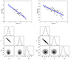 |
Fig. 1. Correlation between luminosity Lb, z and the end time Tb, z. Here we set Ωm = 0.315 and H0 = 67.36 km s−1 Mpc−1 for calculating the luminosity from the measured flux. The data points are the GRBs in X-ray (upper left) and optical samples (upper right). The blue lines correspond to the best-fitting values of the data points with a 95% confidence band. The bottom panels show the 2D posterior contour corner diagrams of the related parameters of the Lb, z − Tb, z correlation for the X-ray (left panel) and optical sample (right panel). |
Best-fitting results of the parameters for different correlations.
4.2. Calibrating the Lb, z − Tb, z correlation
We fix the cosmological parameters Ωm and H0 when deriving the Lb, z − Tb, z correlation in the previous section due to the lack of low-redshift GRBs (z < 0.1), which is related to the circularity problem (Wang et al. 2015). Several approaches to resolving the circularity problem have been suggested (Capozziello & Izzo 2008; Kodama et al. 2008; Liang et al. 2008; Wang & Dai 2011; Wang et al. 2016; Amati et al. 2019; Muccino et al. 2021; Wang et al. 2022). Here, we follow the model-independent method used by Wang et al. (2022), which uses the 36 Hubble parameter data sets H(z) (0.07 < z < 2.36) compiled by Yu et al. (2018) to calibrate the Lb, z − Tb, z correlation. Table 2 presents the comprehensive 36 H(z) data sets obtained using the following methods: the cosmic chronometric technique, the BAO signal in the galaxy distribution, and the BAO signal in the Lyα forest distribution alone or cross-correlated with the quasars (QSOs) method. Typically, there are two steps in the calibration process. First, a continuous function H(z) is constructed from the H(z) data using the GP method, which is then used to calibrate the luminosity distances of low-redshift GRBs in order to calculate Lb, z according to Eq. (7). Second, the model-independent distance modulus of GRBs is calculated using the calibrated correlation parameters.
Hubble parameter data.
We used the public code GaPP (Rasmussen et al. 2006; Seikel et al. 2012) to perform the GP regression process and reconstruct the continuous function H(z). Our program employs a Matern kernel and a smoothness parameter of nu = 1.5. We set the length-scale boundaries parameter to (0.1, 10.0), which ensures that the length-scale values remain within this specified interval, resulting in a smoother kernel. We fit GP models with maximum likelihood estimation (MLE) using the fit function in the package GaussianProcessRegressor1, and the fitted model can be used to make predictions. Then, using the predict function, we finally obtain a smooth H(z) reconstruction curve. After determination of the Hubble parameter H(zi) using the obtained continuous function H(z), one can obtain the corresponding luminosity distance dL(zi) with
 (12)
(12)
The reconstructed H(z) is plotted in Fig. 2, from which we can obtain Lb, z corresponding to low redshifts, which can then be used to fit the parameters “a” and “b” in the Lb, z − Tb, z correlation. In view of the redshift range of the 36 H(z) data sets, 0.17 < z < 2.36, the reconstructed continuous function can only effectively calibrate GRBs for z ≲ 2.50. Taking this into account, we divided the X-ray and optical samples into two subsamples with a boundary of z = 2.50, including 14 and 38 GRBs in low-redshift X-ray and optical samples, respectively. The fitting results are shown in Table 1. We find the calibrated correlation parameters to be consistent with those obtained with all the data in the X-ray and optical samples, respectively.
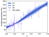 |
Fig. 2. Reconstructed smooth H(z) function (the black line) obtained using the GP method. The shaded regions correspond to the errors of 1σ, 2σ, and 3σ. The points are 36 H(z) data points in the range of 0.07 < z < 2.36. (Source: Fig. 4 in Hu et al. 2021.) |
4.3. Fitting the Lb, z − Tb, z − Ep, i correlation
Including the spectral peak energy Ep, i, Izzo et al. 2015 proposed the three-parameter correlation Lb, z − Tb, z − Ep, i. Here, Ep, i is related to the observed peak energy Ep, obs in the νFν spectrum, Ep, i = Ep, obs × (1 + z). The related data are collected from the literature: Si et al. (2018), Minaev & Pozanenko (2020), Xu et al. (2021) and Lan et al. (2021)2. Si et al. (2018) confirmed the correlation of Lb, z, Tb, z, and Ep, i using selected optical samples. As mentioned above, for the 3D Dinotti correlation, Dainotti et al. (2022a) suggested that the optical samples can be used as effectively as X-ray samples as cosmological probes. Based on 121 long GRBs, Xu et al. (2021) pointed out that the de-evolved L − T − Ep correlation can be used as a standard candle to constrain cosmological parameters. For our purposes, the three-parameter correlation can be written as
 (13)
(13)
The best-fit values of the parameters a, b, c, and the internal dispersion σint in the correlation can be obtained from the likelihood function,
![Mathematical equation: $$ \begin{aligned} \begin{split} \mathcal{L} (a,b,c,\sigma _{\rm int})&\propto \prod _i\frac{1}{\sqrt{\sigma _{\rm int}^2 + \sigma _{y_i}^2 + b^2\sigma _{x_{1,i}}^2 + c^2\sigma _{x_{2,i}}^2}} \\&\times \mathrm{exp}[-\frac{{y_i - a - bx_{1,i} - cx_{2,i}}^2}{2(\sigma _{\rm int}^2 + \sigma _{y_i}^2 + b^2\sigma _{x_{1,i}}^2 + c^2\sigma _{x_{2,i}}^2)}], \end{split} \end{aligned} $$](/articles/aa/full_html/2024/09/aa48542-23/aa48542-23-eq14.gif) (14)
(14)
where x1 = log(Tb, z/s), x2 = log(Ep,j/keV) and y = log(Lb, z/erg s−1). The final constraints are shown in Table 1. The correlations between the three parameters and the posterior distribution of the parameters are plotted in Fig. 3. For the same samples, the internal dispersion σint for the three-parameter correlation is smaller than that for the two-parameter correlation, indicating that the Lb, z − Tb, z − Ep, i correlation for optical samples could be applied in cosmological research as a standard candle.
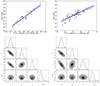 |
Fig. 3. Correlation between luminosity Lb, z, the end time Tb, z, and the spectral peak energy Ep, i. Here we set Ωm = 0.315 and H0 = 67.36 km s−1 Mpc−1 for our calculations. The data points are the GRBs in the X-ray (upper left) and optical samples (upper right). The blue line corresponds to the best-fitting values of the data points with a 95% confidence band. The bottom panels show the 2D posterior contour corner diagrams for the X-ray (left panel) and optical samples (right panel). |
4.4. Calibrating the Lb, z − Tb, z − Ep, i correlation
We calibrate the Lb, z − Tb, z − Ep, i correlation using the method described in Sect. 4.2 for our chosen optical and X-ray samples with low redshift (z ≲ 2.50). The best-fit results are listed in Table 1. We find that the best-fit results after calibration are consistent with those obtained using all the GRB X-ray and optical samples. Compared with the case of all GRBs, the internal dispersion of the calibrated two- and three-parameter correlations is only marginally increased. In the following section, we use the calibrated correlations to constrain the related cosmological parameters.
5. Constraints on cosmological parameters
The distance modulus for GRBs can be written as
 (15)
(15)
After obtaining dL for the Lb, z − Tb, z and Lb, z − Tb, z − Ep, i correlations from Eqs. (7), (10), and (13), we can get the appropriate observed distance modulus for the observed data using Eq. (15). For the two-parameter correlation, the corresponding observed distance modulus is
![Mathematical equation: $$ \begin{aligned} \mu _{\rm obs} = \frac{5}{2}\Bigg [a + b\mathrm{log}T_{b,z} - \mathrm{log}\frac{4{\pi }F_b}{1+z}\Bigg ] - 97.45. \end{aligned} $$](/articles/aa/full_html/2024/09/aa48542-23/aa48542-23-eq16.gif) (16)
(16)
For the errors, following previous works (e.g., Wang & Wang 2019; Xu et al. 2021; Wang et al. 2022), we adopt that the physical quantities Lb, z, Tb, z and Ep, i are obtained independently of the observational data. Therefore, the uncertainty of the distance modulus can be written as
![Mathematical equation: $$ \begin{aligned} \begin{split} \sigma _{\rm obs}&= \frac{5}{2}\Bigg [\sigma _{\rm int}^2 + \sigma _a^2 + \sigma _b^2\mathrm{log}^2_{T_{b,z}} + b^2(\frac{\sigma _{T_{b,z}}}{T_{b,z} \mathrm{ln}10})^2 + (\frac{\sigma _{F_b}}{F_b \mathrm{ln}10})^2 \Bigg ]^{1/2}. \end{split} \end{aligned} $$](/articles/aa/full_html/2024/09/aa48542-23/aa48542-23-eq17.gif) (17)
(17)
For the three-parameter correlation, the observed distance modulus is
![Mathematical equation: $$ \begin{aligned} \mu _{\rm obs} = \frac{5}{2}\Bigg [a + b\mathrm{log}T_{b,z} + c\mathrm{log}E_{p,i}-\mathrm{log}\frac{4{\pi }F_b}{(1+z)}\Bigg ] -97.45, \end{aligned} $$](/articles/aa/full_html/2024/09/aa48542-23/aa48542-23-eq18.gif) (18)
(18)
and the uncertainty of the distance modulus can be written as
![Mathematical equation: $$ \begin{aligned} \begin{split} \sigma _{\rm obs}&= \frac{5}{2}\Bigg [\sigma _{\rm int}^2 + \sigma _a^2 + \sigma _b^2\mathrm{log}^2_{T_{b,z}} + b^2(\frac{\sigma _{T_{b,z}}}{T_{b,z}\mathrm{ln}10})^2 + c^2(\frac{\sigma _{E_{p,i}}}{E_{p,i} \mathrm{ln}10})^2 \\&+ (\frac{\sigma _{F_b}}{F_b \mathrm{ln}10})^2 + \sigma _c^2\mathrm{log}^2_{E_{p,i}}\Bigg ]^{1/2}. \end{split} \end{aligned} $$](/articles/aa/full_html/2024/09/aa48542-23/aa48542-23-eq19.gif) (19)
(19)
The distance modulus calculated from the best fit of the calibrated correlations can be used to constrain the cosmological models. Specifically, one can constrain the DE cosmological model by minimizing χ2,
![Mathematical equation: $$ \begin{aligned} \chi ^2= \sum _{j=1}^{N}\frac{\left[\mu _{\rm obs}(z) - \mu _{th}(z,\theta )\right]^2}{\sigma _{\rm obs}^2}, \end{aligned} $$](/articles/aa/full_html/2024/09/aa48542-23/aa48542-23-eq20.gif) (20)
(20)
where N is the number of GRBs in each category. The observed distance modulus μobs(z) can be calculated from Eqs. (16) and (18). Here, μth(z, θ) is the theoretical distance modulus, and θ represents the free parameters to be constrained.
In general, the luminosity distance can be expressed as
![Mathematical equation: $$ \begin{aligned} d_L=\left\{ \begin{array}{lcl} \frac{c(1+z)}{H_0}(-\Omega _k)^{-\frac{1}{2}}\mathrm{sin}\left[(-\Omega _k)^{-\frac{1}{2}}{\int _0^z}\frac{dz}{E(z)}\right]&\,&{\Omega _k < 0}, \\ \frac{c(1+z)}{H_0}{\int _0^z}\frac{dz}{E(z)}&\,&{\Omega _k = 0},\\ \frac{c(1+z)}{H_0}\Omega _k^{-\frac{1}{2}}\mathrm{sinh}\left[\Omega _k^{-\frac{1}{2}}{\int _0^z}\frac{dz}{E(z)}\right]&\,&{\Omega _k > 0}, \end{array} \right. \end{aligned} $$](/articles/aa/full_html/2024/09/aa48542-23/aa48542-23-eq21.gif) (21)
(21)
where E(z) = H(z)/H0 is the expansion rate function of different cosmological models. For the ωCDM model, the free parameters are Ωm0, Ωx0, ω, and H0. For the X1X2CDM model, the free parameters are Ωm0, Ωx1, Ωx2, ω1, ω2, and H0. We use the emcee package of the MCMC method to find constraints on those parameters in the different models. For the MCMC analysis, we used the following priors for the ωCDM model parameters: Ωm0 ∈ [0, 1], Ωx0 ∈ [0, 1], ω ∈ [ − 5, 2], and H0 ∈ [65, 75], and we used Ωm0 ∈ [0, 1], Ωx1 ∈ [0, 1], Ωx2 ∈ [0, 1], ω1 ∈ [ − 5, 2], ω2 ∈ [ − 5, 2], and H0 ∈ [65, 75] for the X1X2CDM model. We also included the SNe Ia samples (Scolnic et al. 2018) to obtain constraints on the cosmological parameters. It is known that the current limit on ω is approximately −1, and here we set a relatively large range of ω1, 2 in order to cover as much parameter space as possible. Many methods can be used to investigate the convergence of the MCMC program, and here we use the autocorrelation time for our purposes. In general, a longer autocorrelation time, necessitating a longer MCMC chain, signifies a stronger connection between the samples and a sluggish rate of convergence, and the convergent MCMC chains have a short time to explore the whole parameter space. We use the sampler.get-autocorr-time function in emcee to calculate the autocorrelation time. We find that the autocorrelation time increases with the number of free parameters. Briefly, the chain discarding the preceding values after ∼300 steps starts randomly exploring the entire posterior distribution. For our purposes, we removed the first few hundred steps and thinned the autocorrelation time by about half (15 steps) to ensure that the data points cover the full posterior distribution in a short time.
Using the Lb, z − Tb, z correlation, we obtain the constraints on the parameters. For a flat ωCDM model with a single component of DE, combining the data of SNe Ia, X-ray, and optical samples, the final results are  ,
,  , and
, and  . For the nonflat ωCDM model, the constraints on the related parameters are
  ,
,  ,
,  , and
, and  . The 1D and 2D distributions of the related parameters are shown in Fig. 4. We also constrained the ωCDM model using the Lb, z − Tb, z − Ep, i correlation. For the flat model, the final constraints are
  ,
,  , and
, and  , and for the non-flat model, the final constraints are
  ,
,  ,
,  , and
, and  . The 1D and 2D distributions of the related parameters are shown in Fig. 5. All of the results are summarized in Table 3. From the results, we note that the EOS parameter is close to the standard value of ω = −1, but the uncertainty is relatively large. In addition, the constraints on the related parameters are consistent with those of Jia et al. (2022).
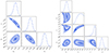 |
Fig. 4. Constraints on the parameters of the ωCDM cosmological model using the SNe Ia data and the Lb, z − Tb, z correlation of X-ray and optical samples of GRBs. The left (right) plot shows the flat (nonflat) ωCDM model. |
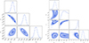 |
Fig. 5. Constraints on the parameters of the ωCDM cosmological model using the SNe Ia data and the Lb, z − Tb, z − Ep, i correlation of X-ray and optical samples of GRBs. The left (right) plot shows the flat (nonflat) ωCDM model. |
Constraints on the cosmological parameters of different models for different GRB samples and correlations.
We also constrained the X1X2CDM model using the Lb, z − Tb, z correlation and the final results can be found in Fig. 6 and Table 3. For flat universe, the constraints are  ,
,  ,
,  ,
,  , and
, and  . For the nonflat X1X2CDM model, the limits are
  ,
,  ,
,  ,
,  ,
,  , and
, and  . Using the Lb, z − Tb, z − Ep, i correlation, with the SNe Ia, X-ray, and optical samples, we obtain
  ,
,  ,
,  ,
,  , and
, and  for the flat model. For nonflat model, we obtain
  ,
,  ,
,  ,
,  ,
,  , and
, and  , which can be seen in Fig. 7 and Table 3. By analyzing the results of the derived data, we find that the error on the equation-of-state parameters of the two-component model ω1 and ω2 is larger than that on the parameter ω in the one-component model, especially the lower-limit error. We can see that the distribution has a long tail when ω is smaller than −1 from the one-dimensional distribution of ω1 and ω2 in Figs. 6 and 7, and the peak distributions of ω1, 2 are around −1 for both flat and nonflat cases. These results are consistent with those shown in Fig. 4 of Gong & Chen (2007).
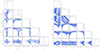 |
Fig. 6. Constraints on the cosmological parameters of the X1X2CDM model using the SNe Ia data and the Lb, z − Tb, z correlation of X-ray and optical samples of GRBs. The left (right) plot shows the flat (nonflat) X1X2CDM model. |
The matter density Ωm0 is almost the same for the one-component and two-component DE models. The one-dimensional histograms of Ωx1 in Figs. 6 and 7 show an additional relatively small peak for the flat two-component DE model. For this model, one have Ωm0 + Ωx1 + Ωx2 = 1, and our results show that Ωm0 is close to 0.3 and the maximum probability of Ωx1 is around 0.6. Then the possible density of Ωx2 is close to 0.1, which should be the optimal solution of the likelihood function. Given the two-component DE model, the optimal solution is likewise satisfied when Ωx2 is close to 0.6 and Ωx1 is close to 0.1. Therefore, there should be a relatively large number of data points at 0.1, resulting in the two peaks in the histogram. These results are consistent with those reported in Figs. 3, 5, and 7 by Gong & Chen (2007).
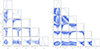 |
Fig. 7. Constraints on the cosmological parameters of the X1X2CDM model using the SNe Ia data and the Lb, z − Tb, z − Ep, i correlation of X-ray and optical samples of GRBs. The left (right) plot shows the flat (nonflat) X1X2CDM model. |
We also combined X-ray and optical samples with SNe Ia data, respectively, to constrain the ωCDM and X1X2CDM models using the two, and three-parameter correlations. All of the results are summarized in Table 3. We find that for each GRB correlation, the constraints on the related parameters are consistent. For the same cosmological model, the Ωm and Ωx constrained using the three-parameter correlation are slightly smaller than those derived from the two-parameter correlation. Although there is a very significant error bar, we note that the peaks in the ω1 and ω2 distributions are similar.
In Fig. 8, we present a Hubble diagram of different GRBs samples calibrated using the Lb, z − Tb, z correlation (left) and the Lb, z − Tb, z − Ep, i correlation (right). It is worth noting that the error bars for the distance modulus derived from the two correlations for high-redshift GRBs are still large. These results suggest that the calibrated correlations of GRBs alone cannot be used to measure the cosmological parameters as precisely as SNe Ia. However, GRBs are valuable for expanding the Hubble diagram to high redshift. We expect that GRBs will be employed as a fully fledged cosmic probe rather than an auxiliary tool when the number of high-redshift observations increases and the precision of forthcoming observations improves.
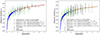 |
Fig. 8. Calibrated GRB Hubble diagram at high redshift using the Lb, z − Tb, z correlation (left-hand panel) and the Lb, z − Tb, z − Ep, i correlation (right-hand panel) with SNe Ia, X-ray, and optical samples. The black and green points represent X-ray and optical samples, respectively. Blue points are SNe Ia from the Pantheon sample. The solid red line corresponds to the theoretical distance modulus calculated for a flat ΛCDM model with H0 = 67.36 km s−1 Mpc−1 and Ωm = 0.315. |
We also used AIC and BIC to compare different models; these can be written as
 (22)
(22)
and
 (23)
(23)
where χ2 is defined in Eq. (20), N is the number of data points, and p is the number of free parameters of the relative model. The model with lower AIC or BIC values is favored by the criterion, and we compute ΔX (where X = AIC or BIC) values with respect to the flat ωCDM model. A negative ΔX suggests that the model under consideration performs better than the reference model. If it is positive, ΔX ∈ [0,2] indicates the model under consideration has substantial support for the reference mode, and ΔX ∈ [2,6] indicates the candidate model is less favored than the reference model. The candidate model is not strongly supported for ΔX > 6. The values of AIC and BIC for ωCDM and X1X2CDM models are shown in Table 3. Comparing the results of the models based on the information criteria, we find that AIC and BIC always favor models with fewer free parameters.
6. Discussion and conclusion
Based on the features of their light curves, we screened GRBs with a plateau phase followed by a decay phase with a decay index of -2. We also screened the optical samples with a plateau and decay phase using the same procedure. It has been suggested that GRBs showing these same characteristics in their light curves are likely to have the same physical origin. Therefore, we acquired both X-ray and optical samples for our studies. We find that the selected optical samples have a compact Lb, z − Tb, z correlation, similar to that found for the X-ray samples selected by Wang et al. (2022). We investigated the Lb, z − Tb, z − Ep, i correlation for the two sets of samples, and find that the internal dispersion (σint) of the three-parameter correlation is smaller than that of the two-parameter correlation for the same sets of samples, indicating that the Lb, z − Tb, z − Ep, i correlation is tighter than the Lb, z − Tb, z correlation.
In order to investigate the potential use of GRBs as a cosmological probe, we applied the GP method to calibrate the two-parameter correlation and obtained the model-independent distance modulus. The MCMC approach was then used to derive the best-fitting results of the calibrated correlations. The σint of the calibrated correlations were found to be slightly larger, which could be due to the fact that GRB samples are smaller at lower redshifts. It is expected that the GRB database will be enlarged in the near future because of an increase in the number of observers entering service, allowing us to do more extensive screening and studies.
Using the calibrated X-ray and optical samples, we constrained the free parameters of the one-component DE model (ωCDM model) and two-component DE model (X1X2CDM model). We find that the selected optical and X-ray sample can effectively constrain the cosmological parameters, showing that careful screening of GRBs is necessary for cosmological purposes. The restriction results of the three-parameter correlation for both groups of samples accord with the two-parameter correlation. The constraints on ω1 and ω2 of the X1X2CDM model are also consistent at 1σ level. This seems to imply that the composition of DE prefers a single component. We also used the AIC and BIC to compare the different models, and find that the model with fewer free parameters is favored.
Compared with previous works (Gong & Chen 2007; Si et al. 2018; Wang et al. 2022; Li et al. 2023c), our study has the following new characteristics: (1) We selected different samples of GRBs that could have the same physical mechanism based on the decay index, and update the constraints on the cosmological parameters of the X1X2CDM model using more SNe Ia and GRBs data. (2) We investigated not only the Lb, z − Tb, z connection existing in the selected GRB data, but also the much tighter Lb, z − Tb, z − Ep, i correlation, and applied both of the correlations to constrain cosmological parameters.
Among them, GRB 190114A was dropped because of poorly constrained Ep, i
Acknowledgments
This work is supported by the National Natural Science Foundation of China (Grant Nos. U2038106 and 12273009), the Shandong Provincial Natural Science Foundation (Grant No. ZR2021MA021), Jiangsu Funding Program for Excellent Postdoctoral Talent (20220ZB59), China Postdoctoral Science Foundation (2022M721561) and China Manned Spaced Project (CMS-CSST-2021-A12).
References
- Akaike, H. 1974, IEEE Trans. Autom. Contr., 19, 716 [Google Scholar]
- Alam, S., Ata, M., Bailey, S., et al. 2017, MNRAS, 470, 2617 [Google Scholar]
- Amati, L., & Della Valle, M. 2013, Int. J. Mod. Phys. D, 22, 1330028 [NASA ADS] [CrossRef] [Google Scholar]
- Amati, L., Frontera, F., Tavani, M., et al. 2002, A&A, 390, 81 [NASA ADS] [CrossRef] [EDP Sciences] [Google Scholar]
- Amati, L., Guidorzi, C., Frontera, F., et al. 2008, MNRAS, 391, 577 [Google Scholar]
- Amati, L., D’Agostino, R., Luongo, O., et al. 2019, MNRAS, 486, L46 [Google Scholar]
- Bloom, J. S., Frail, D. A., & Sari, R. 2001, AJ, 121, 2879 [NASA ADS] [CrossRef] [Google Scholar]
- Cao, S., Dainotti, M., & Ratra, B. 2022a, MNRAS, 516, 1386 [NASA ADS] [CrossRef] [Google Scholar]
- Cao, S., Dainotti, M., & Ratra, B. 2022b, MNRAS, 512, 439 [NASA ADS] [CrossRef] [Google Scholar]
- Cao, S., Khadka, N., & Ratra, B. 2022c, MNRAS, 510, 2928 [NASA ADS] [CrossRef] [Google Scholar]
- Cao, S., Ryan, J., Khadka, N., et al. 2021, MNRAS, 501, 1520 [Google Scholar]
- Copeland, E. J., Sami, M., & Tsujikawa, S. 2006, Int. J. Mod. Phys. D, 15, 1753 [NASA ADS] [CrossRef] [Google Scholar]
- Capozziello, S., & Izzo, L. 2008, A&A, 490, 31 [NASA ADS] [CrossRef] [EDP Sciences] [Google Scholar]
- Cardone, V. F., Capozziello, S., & Dainotti, M. G. 2009, MNRAS, 391, L79 [NASA ADS] [Google Scholar]
- Cardone, V. F., Dainotti, M. G., Capozziello, S., et al. 2010, MNRAS, 408, 1181 [NASA ADS] [CrossRef] [Google Scholar]
- Carroll, S. M. 2001, Liv. Rev. Relativ., 4, 1 [NASA ADS] [CrossRef] [Google Scholar]
- Cucchiara, A., Levan, A. J., Fox, D. B., et al. 2011, ApJ, 736, 7 [Google Scholar]
- D’Agostini, G. 2005, ArXiv e-prints [arXiv: physics/0511182] [Google Scholar]
- Dai, Z. G., & Lu, T. 1998a, Phys. Rev. Lett., 81, 4301 [NASA ADS] [CrossRef] [Google Scholar]
- Dai, Z. G., & Lu, T. 1998b, A&A, 333, L87 [NASA ADS] [Google Scholar]
- Dai, Z. G., Liang, E. W., & Xu, D. 2004, ApJ, 612, L101 [NASA ADS] [CrossRef] [Google Scholar]
- Dainotti, M. G., Cardone, V. F., & Capozziello, S. 2008, MNRAS, 391, L79 [NASA ADS] [CrossRef] [Google Scholar]
- Dainotti, M. G., Willingale, R., Capozziello, S., et al. 2010, ApJ, 722, L215 [NASA ADS] [CrossRef] [Google Scholar]
- Dainotti, M. G., Fabrizio Cardone, V., Capozziello, S., et al. 2011, ApJ, 730, 135 [NASA ADS] [CrossRef] [Google Scholar]
- Dainotti, M. G., Cardone, V. F., Piedipalumbo, E., et al. 2013, MNRAS, 436, 82 [NASA ADS] [CrossRef] [Google Scholar]
- Dainotti, M. G., Petrosian, V., & Bowden, L. 2021, ApJ, 914, L40 [NASA ADS] [CrossRef] [Google Scholar]
- Dainotti, M. G., Nielson, V., Sarracino, G., et al. 2022a, MNRAS, 514, 1828 [CrossRef] [Google Scholar]
- Dainotti, M. G., Sarracino, G., & Capozziello, S. 2022b, PASJ, 74, 1095 [NASA ADS] [CrossRef] [Google Scholar]
- Dainotti, M. G., Lenart, A. Ł., Chraya, A., et al. 2023, MNRAS, 518, 2201 [Google Scholar]
- Delubac, T., Bautista, J. E., Busca, N. G., et al. 2015, A&A, 574, A59 [NASA ADS] [CrossRef] [EDP Sciences] [Google Scholar]
- Deng, C., Huang, Y.-F., & Xu, F. 2023, ApJ, 943, 126 [NASA ADS] [CrossRef] [Google Scholar]
- Du, M., Yi, S.-X., Liu, T., et al. 2021, ApJ, 908, 242 [NASA ADS] [CrossRef] [Google Scholar]
- Durrer, R., & Maartens, R. 2008, Gen. Rel. Grav., 40, 301 [Google Scholar]
- Eisenstein, D. J., Zehavi, I., Hogg, D. W., et al. 2005, ApJ, 633, 560 [Google Scholar]
- Fan, Y.-Z., & Xu, D. 2006, MNRAS, 372, L19 [NASA ADS] [CrossRef] [Google Scholar]
- Font-Ribera, A., Kirkby, D., Busca, N., et al. 2014, JCAP, 2014, 027 [Google Scholar]
- Foreman-Mackey, D., Hogg, D. W., Lang, D., et al. 2013, PASP, 125, 306 [NASA ADS] [CrossRef] [Google Scholar]
- Frieman, J. A., Turner, M. S., & Huterer, D. 2008, ARA&A, 46, 385 [Google Scholar]
- Gehrels, N., Ramirez-Ruiz, E., & Fox, D. B. 2009, ARA&A, 47, 567 [NASA ADS] [CrossRef] [Google Scholar]
- Ghirlanda, G., Ghisellini, G., Lazzati, D., et al. 2004a, ApJ, 613, L13 [Google Scholar]
- Ghirlanda, G., Ghisellini, G., & Lazzati, D. 2004b, ApJ, 616, 331 [Google Scholar]
- Ghirlanda, G., Ghisellini, G., & Firmani, C. 2006, New J. Phys., 8, 123 [CrossRef] [Google Scholar]
- Gong, Y., & Chen, X. 2007, Phys. Rev. D, 76, 123007 [CrossRef] [Google Scholar]
- Hu, J. P., & Wang, F. Y. 2022, A&A, 661, A71 [NASA ADS] [CrossRef] [EDP Sciences] [Google Scholar]
- Hu, J. P., Wang, F. Y., & Dai, Z. G. 2021, MNRAS, 507, 730 [NASA ADS] [CrossRef] [Google Scholar]
- Izzo, L., Muccino, M., Zaninoni, E., et al. 2015, A&A, 582, A115 [NASA ADS] [CrossRef] [EDP Sciences] [Google Scholar]
- Jia, X. D., Hu, J. P., Yang, J., et al. 2022, MNRAS, 516, 2575 [Google Scholar]
- Jimenez, R., & Loeb, A. 2002, ApJ, 573, 37 [NASA ADS] [CrossRef] [Google Scholar]
- Jimenez, R., Verde, L., Treu, T., et al. 2003, ApJ, 593, 622 [NASA ADS] [CrossRef] [Google Scholar]
- Khadka, N., Luongo, O., Muccino, M., et al. 2021, JCAP, 2021, 042 [Google Scholar]
- Klebesadel, R. W., Strong, I. B., & Olson, R. A. 1973, ApJ, 182, L85 [NASA ADS] [CrossRef] [Google Scholar]
- Kodama, Y., Yonetoku, D., Murakami, T., et al. 2008, MNRAS, 391, L1 [NASA ADS] [CrossRef] [Google Scholar]
- Kouveliotou, C., Meegan, C. A., Fishman, G. J., et al. 1993, ApJ, 413, L101 [NASA ADS] [CrossRef] [Google Scholar]
- Kumar, P., & Zhang, B. 2015, Phys. Rep., 561, 1 [Google Scholar]
- Lamb, D. Q., & Reichart, D. E. 2000, ApJ, 536, 1 [Google Scholar]
- Lan, G.-X., Wei, J.-J., Zeng, H.-D., et al. 2021, MNRAS, 508, 52 [CrossRef] [Google Scholar]
- Lasky, P. D., & Glampedakis, K. 2016, MNRAS, 458, 1660 [NASA ADS] [CrossRef] [Google Scholar]
- Levine, D., Dainotti, M., Zvonarek, K. J., et al. 2022, ApJ, 925, 15 [NASA ADS] [CrossRef] [Google Scholar]
- Li, L., Liang, E.-W., Tang, Q.-W., et al. 2012, ApJ, 758, 27 [NASA ADS] [CrossRef] [Google Scholar]
- Li, Z., Zhang, B., & Liang, N. 2023a, MNRAS, 521, 4406 [CrossRef] [Google Scholar]
- Li, X.-J., Zhang, W.-L., Yi, S.-X., et al. 2023b, ApJS, 265, 56 [NASA ADS] [CrossRef] [Google Scholar]
- Li, J.-L., Yang, Y.-P., Yi, et al. 2023c, ApJ, 953, 58 [NASA ADS] [CrossRef] [Google Scholar]
- Liang, E., & Zhang, B. 2005, ApJ, 633, 611 [Google Scholar]
- Liang, E., & Zhang, B. 2006, MNRAS, 369, L37 [NASA ADS] [CrossRef] [Google Scholar]
- Liang, E.-W., Zhang, B.-B., & Zhang, B. 2007, ApJ, 670, 565 [Google Scholar]
- Liang, N., Xiao, W. K., Liu, Y., et al. 2008, ApJ, 685, 354 [Google Scholar]
- Liang, N., Li, Z., Xie, X., et al. 2022, ApJ, 941, 84 [CrossRef] [Google Scholar]
- Liu, Y., Liang, N., Xie, X., et al. 2022, ApJ, 935, 7 [NASA ADS] [CrossRef] [Google Scholar]
- Lü, H.-J., & Zhang, B. 2014, ApJ, 785, 74 [CrossRef] [Google Scholar]
- Mészáros, P. 2006, Rep. Prog. Phys., 69, 2259 [CrossRef] [Google Scholar]
- Metzger, B. D., Giannios, D., Thompson, T. A., et al. 2011, MNRAS, 413, 2031 [NASA ADS] [CrossRef] [Google Scholar]
- Minaev, P. Y., & Pozanenko, A. S. 2020, MNRAS, 492, 1919 [NASA ADS] [CrossRef] [Google Scholar]
- Moresco, M. 2015, MNRAS, 450, L16 [NASA ADS] [CrossRef] [Google Scholar]
- Moresco, M., Cimatti, A., Jimenez, R., et al. 2012, JCAP, 2012, 006 [CrossRef] [Google Scholar]
- Moresco, M., Pozzetti, L., Cimatti, A., et al. 2016, JCAP, 2016, 014 [CrossRef] [Google Scholar]
- Muccino, M., Izzo, L., Luongo, O., et al. 2021, ApJ, 908, 181 [Google Scholar]
- Nousek, J. A., Kouveliotou, C., Grupe, D., et al. 2006, ApJ, 642, 389 [Google Scholar]
- O’Brien, P. T., Willingale, R., Osborne, J., et al. 2006, ApJ, 647, 1213 [NASA ADS] [CrossRef] [Google Scholar]
- Ong, Y. C. 2023, Universe, 9, 437 [NASA ADS] [CrossRef] [Google Scholar]
- Pavlov, A., Westmoreland, S., Saaidi, K., et al. 2013, Phys. Rev. D, 88, 123513 [NASA ADS] [CrossRef] [Google Scholar]
- Peebles, P. J. E., & Ratra, B. 1988, ApJ, 325, L17 [NASA ADS] [CrossRef] [Google Scholar]
- Perlmutter, S., Aldering, G., Goldhaber, G., et al. 1999, ApJ, 517, 565 [Google Scholar]
- Planck Collaboration XVI. 2014, A&A, 571, A16 [NASA ADS] [CrossRef] [EDP Sciences] [Google Scholar]
- Planck Collaboration XIII. 2016, A&A, 594, A13 [NASA ADS] [CrossRef] [EDP Sciences] [Google Scholar]
- Planck Collaboration VI. 2020, A&A, 641, A6 [NASA ADS] [CrossRef] [EDP Sciences] [Google Scholar]
- Postnikov, S., Dainotti, M. G., Hernandez, X., et al. 2014, ApJ, 783, 126 [NASA ADS] [CrossRef] [Google Scholar]
- Qin, Y., Liang, E.-W., Liang, Y.-F., et al. 2013, ApJ, 763, 15 [NASA ADS] [CrossRef] [Google Scholar]
- Rasmussen, C. E., & Williams, C. K. I. 2006, in Gaussian Processes for Machine Learning, eds. C. E. Rasmussen, & C. K. I. Williams [Google Scholar]
- Ratra, B., & Peebles, P. J. E. 1988, Phys. Rev. D, 37, 3406 [Google Scholar]
- Ratsimbazafy, A. L., Loubser, S. I., Crawford, S. M., et al. 2017, MNRAS, 467, 3239 [NASA ADS] [CrossRef] [Google Scholar]
- Riess, A. G., Filippenko, A. V., Challis, P., et al. 1998, AJ, 116, 1009 [Google Scholar]
- Rowlinson, A., O’Brien, P. T., Metzger, B. D., et al. 2013, MNRAS, 430, 1061 [NASA ADS] [CrossRef] [Google Scholar]
- Schaefer, B. E. 2007, ApJ, 660, 16 [Google Scholar]
- Schwarz, G. 1978, Ann. Stat., 6, 461 [Google Scholar]
- Scolnic, D. M., Jones, D. O., Rest, A., et al. 2018, ApJ, 859, 101 [NASA ADS] [CrossRef] [Google Scholar]
- Seikel, M., Clarkson, C., & Smith, M. 2012, JCAP, 2012, 036 [CrossRef] [Google Scholar]
- Si, S.-K., Qi, Y.-Q., Xue, F.-X., et al. 2018, ApJ, 863, 50 [NASA ADS] [CrossRef] [Google Scholar]
- Simon, J., Verde, L., & Jimenez, R. 2005, Phys. Rev. D, 71, 123001 [NASA ADS] [CrossRef] [Google Scholar]
- Spergel, D. N., Verde, L., Peiris, H. V., et al. 2003, ApJS, 148, 175 [Google Scholar]
- Stern, D., Jimenez, R., Verde, L., et al. 2010, JCAP, 2010, 008 [CrossRef] [Google Scholar]
- Tang, C.-H., Huang, Y.-F., Geng, J.-J., et al. 2019, ApJS, 245, 1 [NASA ADS] [CrossRef] [Google Scholar]
- Tian, X., Li, J.-L., Yi, S.-X., et al. 2023, ApJ, 958, 74 [NASA ADS] [CrossRef] [Google Scholar]
- Wang, F. Y., & Dai, Z. G. 2011, A&A, 536, A96 [NASA ADS] [CrossRef] [EDP Sciences] [Google Scholar]
- Wang, Y. Y., & Wang, F. Y. 2019, ApJ, 873, 39 [Google Scholar]
- Wang, F.-Y., Qi, S., & Dai, Z.-G. 2011, MNRAS, 415, 3423 [NASA ADS] [CrossRef] [Google Scholar]
- Wang, F. Y., Dai, Z. G., & Liang, E. W. 2015, New A Rv., 67, 1 [NASA ADS] [CrossRef] [Google Scholar]
- Wang, J. S., Wang, F. Y., Cheng, K. S., et al. 2016, A&A, 585, A68 [NASA ADS] [CrossRef] [EDP Sciences] [Google Scholar]
- Wang, F. Y., Hu, J. P., Zhang, G. Q., et al. 2022, ApJ, 924, 97 [NASA ADS] [CrossRef] [Google Scholar]
- Wei, J.-J., & Wu, X.-F. 2017, Int. J. Mod. Phys. D, 26, 1730002 [NASA ADS] [CrossRef] [Google Scholar]
- Wei, J., Wu, X., Wang, F., et al. 2018, Sci. Sin. Phys. Mech. Astron., 48, 039505 [NASA ADS] [CrossRef] [Google Scholar]
- Willingale, R., O’Brien, P. T., Osborne, J. P., et al. 2007, ApJ, 662, 1093 [NASA ADS] [CrossRef] [Google Scholar]
- Xu, F., Tang, C.-H., Geng, J.-J., et al. 2021, ApJ, 920, 135 [NASA ADS] [CrossRef] [Google Scholar]
- Yi, S.-X., Wu, X.-F., Wang, F.-Y., et al. 2015, ApJ, 807, 92 [NASA ADS] [CrossRef] [Google Scholar]
- Yi, S.-X., Xi, S.-Q., Yu, H., et al. 2016, ApJS, 224, 20 [NASA ADS] [CrossRef] [Google Scholar]
- Yi, S.-X., Wu, X.-F., Zou, Y.-C., et al. 2020, ApJ, 895, 94 [NASA ADS] [CrossRef] [Google Scholar]
- Yi, S.-X., Xie, W., Ma, S.-B., et al. 2021, MNRAS, 507, 1047 [NASA ADS] [CrossRef] [Google Scholar]
- Yi, S.-X., Du, M., & Liu, T. 2022, ApJ, 924, 69 [NASA ADS] [CrossRef] [Google Scholar]
- Yonetoku, D., Murakami, T., Nakamura, T., et al. 2004, ApJ, 609, 935 [Google Scholar]
- Yu, H., Ratra, B., & Wang, F.-Y. 2018, ApJ, 856, 3 [NASA ADS] [CrossRef] [Google Scholar]
- Zhao, W., Zhang, J.-C., Zhang, Q.-X., et al. 2020, ApJ, 900, 112 [NASA ADS] [CrossRef] [Google Scholar]
- Zhang, B., & Mészáros, P. 2001, ApJ, 552, L35 [CrossRef] [Google Scholar]
- Zhang, B., Fan, Y. Z., Dyks, J., et al. 2006, ApJ, 642, 354 [Google Scholar]
- Zhang, C., Zhang, H., Yuan, S., et al. 2014, Res. Astron. Astrophys., 14, 1221 [CrossRef] [Google Scholar]
All Tables
Constraints on the cosmological parameters of different models for different GRB samples and correlations.
All Figures
|
Fig. 1. Correlation between luminosity Lb, z and the end time Tb, z. Here we set Ωm = 0.315 and H0 = 67.36 km s−1 Mpc−1 for calculating the luminosity from the measured flux. The data points are the GRBs in X-ray (upper left) and optical samples (upper right). The blue lines correspond to the best-fitting values of the data points with a 95% confidence band. The bottom panels show the 2D posterior contour corner diagrams of the related parameters of the Lb, z − Tb, z correlation for the X-ray (left panel) and optical sample (right panel). |
| In the text | |
|
Fig. 2. Reconstructed smooth H(z) function (the black line) obtained using the GP method. The shaded regions correspond to the errors of 1σ, 2σ, and 3σ. The points are 36 H(z) data points in the range of 0.07 < z < 2.36. (Source: Fig. 4 in Hu et al. 2021.) |
| In the text | |
|
Fig. 3. Correlation between luminosity Lb, z, the end time Tb, z, and the spectral peak energy Ep, i. Here we set Ωm = 0.315 and H0 = 67.36 km s−1 Mpc−1 for our calculations. The data points are the GRBs in the X-ray (upper left) and optical samples (upper right). The blue line corresponds to the best-fitting values of the data points with a 95% confidence band. The bottom panels show the 2D posterior contour corner diagrams for the X-ray (left panel) and optical samples (right panel). |
| In the text | |
|
Fig. 4. Constraints on the parameters of the ωCDM cosmological model using the SNe Ia data and the Lb, z − Tb, z correlation of X-ray and optical samples of GRBs. The left (right) plot shows the flat (nonflat) ωCDM model. |
| In the text | |
|
Fig. 5. Constraints on the parameters of the ωCDM cosmological model using the SNe Ia data and the Lb, z − Tb, z − Ep, i correlation of X-ray and optical samples of GRBs. The left (right) plot shows the flat (nonflat) ωCDM model. |
| In the text | |
|
Fig. 6. Constraints on the cosmological parameters of the X1X2CDM model using the SNe Ia data and the Lb, z − Tb, z correlation of X-ray and optical samples of GRBs. The left (right) plot shows the flat (nonflat) X1X2CDM model. |
| In the text | |
|
Fig. 7. Constraints on the cosmological parameters of the X1X2CDM model using the SNe Ia data and the Lb, z − Tb, z − Ep, i correlation of X-ray and optical samples of GRBs. The left (right) plot shows the flat (nonflat) X1X2CDM model. |
| In the text | |
|
Fig. 8. Calibrated GRB Hubble diagram at high redshift using the Lb, z − Tb, z correlation (left-hand panel) and the Lb, z − Tb, z − Ep, i correlation (right-hand panel) with SNe Ia, X-ray, and optical samples. The black and green points represent X-ray and optical samples, respectively. Blue points are SNe Ia from the Pantheon sample. The solid red line corresponds to the theoretical distance modulus calculated for a flat ΛCDM model with H0 = 67.36 km s−1 Mpc−1 and Ωm = 0.315. |
| In the text | |
Current usage metrics show cumulative count of Article Views (full-text article views including HTML views, PDF and ePub downloads, according to the available data) and Abstracts Views on Vision4Press platform.
Data correspond to usage on the plateform after 2015. The current usage metrics is available 48-96 hours after online publication and is updated daily on week days.
Initial download of the metrics may take a while.