| Issue |
A&A
Volume 684, April 2024
|
|
|---|---|---|
| Article Number | A16 | |
| Number of page(s) | 16 | |
| Section | Interstellar and circumstellar matter | |
| DOI | https://doi.org/10.1051/0004-6361/202347808 | |
| Published online | 29 March 2024 | |
The evolution of continuum polarization in type II supernovae as a diagnostic of ejecta morphology
1
Institut d’Astrophysique de Paris, CNRS-Sorbonne Université,
98 bis boulevard Arago,
75014
Paris, France
e-mail: This email address is being protected from spambots. You need JavaScript enabled to view it.
2
Department of Physics and Astronomy & Pittsburgh Particle Physics, Astrophysics, and Cosmology Center (PITT PACC), University of Pittsburgh,
3941 O’Hara Street,
Pittsburgh, PA
15260, USA
3
Department of Astronomy, San Diego State University,
San Diego, CA
92182-1221, USA
Received:
26
August
2023
Accepted:
14
January
2024
Abstract
The linear polarization of the optical continuum of type II supernovae (SNe), together with its temporal evolution is a promising source of information about the large-scale geometry of their ejecta. To help access this information, we undertook 2D polarized radiative transfer calculations to map the possible landscape of type II SN continuum polarization (Pcont) from 20 to 300 days after explosion. Our simulations were based on crafted 2D axisymmetric ejecta constructed from 1D nonlocal thermodynamic equilibrium time-dependent radiative transfer calculations for the explosion of a red supergiant star. Following the approach used in our previous work on SN 2012aw, we considered a variety of bipolar explosions in which spherical symmetry is broken by material within ~30° of the poles that has a higher kinetic energy (up to a factor of two) and higher 56Ni abundance (up to a factor of about five, allowing for 56Ni at high velocity). Our set of eight 2D ejecta configurations produced considerable diversity in Pcont (λ ~ 7000 Å), although its maximum of 1–4% systematically occurs around the transition to the nebular phase. Before and after this transition, Pcont may be null, constant, rising, or decreasing, which is caused by the complex geometry of the depth-dependent density and ionization and also by optical depth effects. Our modest angle-dependent explosion energy can yield a Pcont of 0.5–1% at early times. Residual optical-depth effects can yield an angle-dependent SN brightness and constant polarization at nebular times. The observed values of Pcont tend to be lower than obtained here. This suggests that more complicated geometries with competing large-scale structures cancel the polarization. Extreme asymmetries seem to be excluded.
Key words: polarization / radiative transfer / supernovae: general
© The Authors 2024
 Open Access article, published by EDP Sciences, under the terms of the Creative Commons Attribution License (https://creativecommons.org/licenses/by/4.0), which permits unrestricted use, distribution, and reproduction in any medium, provided the original work is properly cited.
This article is published in open access under the Subscribe to Open model. This email address is being protected from spambots. You need JavaScript enabled to view it. to support open access publication.
1 Introduction
A fundamental property of the neutrino-driven explosion mechanism of massive stars is its inherently multidimensional character (see, e.g., Bollig et al. 2021; Mezzacappa et al. 2020; O’Connor & Couch 2018; Vartanyan et al. 2022). Although this asymmetry may leave an imprint on the supernova (SN) light curve and spectra, its most unambiguous signature in nonspatially resolved ejecta is a residual nonzero linear polarization (Shapiro & Sutherland 1982; Wang & Wheeler 2008).
Polarization studies of SNe started in earnest with the type II-peculiar SN 1987A, with multiband polarimetry (e.g., Mendez et al. 1988) and spectropolarimetry (e.g., Cropper et al. 1988). Hoflich (1991) and Jeffery (1991) modeled the intrinsic linear polarization of SN 1987A and proposed that it originates from electron scattering in an asymmetric ejecta. The polarization is understood to arise from an aspherical scattering photosphere. Chugai (1992) proposed that an asymmetric distribution of 56Ni could also be the source of the SN 1987A polarization. Because of the scarcity of type II-peculiar SNe such as 1987A among non-interacting type II SNe, recent spectropolarimetric observations have instead primarily been gathered for type II-plateau (II-P) SNe. The first complete coverage of the spectropolarimetric evolution of a type II-P SN was obtained for 2004dj (Leonard et al. 2006), which revealed a low intrinsic continuum polarization through the plateau phase, which then spiked at the onset of the nebular phase and subsequently followed a 1/t2 drop. While this naively appeared to imply a greater asymmetry of the inner ejecta relative to the outer ejecta, Dessart & Hillier (2011b) found that the polarization peak is in part driven by the transition from a multiple- to a single-scattering regime, hence a radiative transfer effect. This was later confirmed with the simulations of Dessart et al. (2021b) for SN 2012aw with more consistent models that covered the full evolution of a 2D ejecta from the photospheric to the nebular phase. This behavior is not generic, however, because SNe II-P exhibit a variety of behavior (e.g., Chornock et al. 2010; Leonard et al. 2012b), with low polarization at all times (e.g., SN 1999em, Leonard et al. 2001), a polarization peak before the end of the plateau phase (e.g., SN 2013ej, Leonard et al. 2015; Mauerhan et al. 2017; Nagao et al. 2021; see also SN 2017gmr, Nagao et al. 2019), or nearly constant polarization at nebular times (e.g., SNe 2008bk or 2013ej, Leonard et al. 2012a, Leonard et al. 2015).
The hypothesis that the inner ejecta of type II SNe is asymmetric is indirectly supported by the detection of nonzero polarization in stripped-envelope SNe. These objects lack a massive H-rich envelope to inhibit the expansion of the metal-rich asymmetric core. Although the absence of hydrogen reduces the importance of electron scattering in favor of line opacity and therefore complicates the interpretation of the polarization signatures, intrinsic linear polarization has been routinely detected in type IIb SNe (e.g., SN 1993J, Trammell et al. 1993; SN 2008ax, Chornock et al. 2011), type Ib SNe (e.g., SN 2008D, Maund et al. 2009), type Ic SNe (e.g., SN 2007gr, Tanaka et al. 2008), and even broad-line type Ic SNe (e.g., SN 2002ap, Leonard et al. 2002).
These polarization measures suggest an asymmetry of the explosion that causes an asymmetric density distribution (Hoflich 1991; Jeffery 1991; Dessart & Hillier 2011b) or an asymmetric distribution of the 56Ni (Chugai 2006; Dessart et al. 2021a; Leonard et al. 2021). Because the 56Ni mass scales with the explosion energy1, the ejecta asymmetry is probably caused by a combination of both effects. Dessart & Hillier (2011b) emphasized that an asymmetric density distribution does not just impact the distribution of the free electrons that scatter the radiation, but also the distribution of the escaping flux as observed on the plane of the sky. Since radiation tends to escape from regions of lower optical depth, an oblate distribution of free electrons may induce a prolate distribution of the escaping flux and produce a complicated polarization signature. A globally consistent model of the polarization is therefore necessary, especially at times when the ejecta are optically thick. Hence, in order to improve the physical realism of the initial conditions for these spectropolarimetric modeling studies, Dessart et al. (2021b) set up a 2D axially symmetric ejecta using physically consistent 1D nonlocal-thermodynamic equilibrium (non-LTE) radiative transfer calculations computed with CMFGEN (Hillier & Dessart 2012) and started from radiation-hydrodynamics models of the explosion. Post-processing with the 2D polarized radiative transfer code LONG_POL (Hillier 1994, 1996; Dessart & Hillier 2011b) showed that an asymmetric explosion of a standard type II-P SN may explain the photometric, spectroscopic, and multiwavelength polarization evolution of a SN like 2012aw (Dessart et al. 2021b).
In this study, we consider a broad variety of 2D axisymmetric but aspherical ejecta and explore the evolution in the continuum polarization from early times in the photospheric phase until 300 days in the nebular phase. We consider variations in kinetic energy and 56Ni mass with angle, including various combinations thereof, which therefore imply radial variations in both density and 56Ni mass fraction with angle. In particular, we aim to address the origin of high polarization at early epochs, the range of polarization peaks attained, the behavior at late times, and importantly, we wish to understand what drives this diversity. In the next section, we present our numerical setup for the 1D CMFGEN simulations and the 2D LONG_POL simulations. The grid of models is composed of ejecta with a range of kinetic energies and 56Ni mass, invoking the presence of 56Ni at low or high velocity. In Sect. 3 we describe the results for a representative model in detail. In Sect. 4, we describe the results for the full set of 2D models, addressing the physical conditions that produce the different evolution of the continuum polarization in turn. We present our conclusions in Sect. 52.
2 Numerical setup
The calculations presented in this work were performed in two steps. We first generated 1D explosion models for which we computed the evolution until 300 days with CMFGEN (Sect. 2.1). The second step was to build 2D axisymmetric ejecta by combining different pairs of 1D ejecta. For each of these pairs, we computed the 2D polarized radiative transfer with LONG_POL (Sect. 2.2) and extracted the continuum polarization at multiple epochs. Since a separate project was to analyze our VLT-FORS3 spectropolarimetric data for SN 2008bk (see the preliminary results in Leonard et al. 2012a, 2015), we chose for this work a 12 M⊙ progenitor producing a low-energy explosion (Lisakov et al. 2017). In this way, the set of simulations here may also be used for the analysis of the SN 2008bk spectropolarimetry.
2.1 Spherically symmetric calculations with CMFGEN
All simulations in this work are based on a nonrotating 12 M⊙ star initially and evolved at solar metallicity4 until core collapse (i.e., when the maximum Fe-core infall velocity exceeds 1000 km s−1) with the code MESA version 10108 (Paxton et al. 2011, 2013, 2015, 2018). The default parameters were used, except for a reduced wind mass-loss rate relative to the Dutch recipe (we adopted a scaling of 0.6). As in our previous works (see, e.g., Dessart et al. 2013), we increased the mixing-length parameter to three to produce a relatively compact red supergiant star at collapse. At core collapse, the model has a luminosity of 56700 L⊙, a surface radius of 485 R⊙, an effective temperature of 4040 K, a total mass of 10.34 M⊙, an H-rich envelope mass of 7.03 M⊙, a He core mass of 3.31 M⊙, and an Fe core mass of 1.5 M⊙ (as defined by the innermost envelope location where the electron fraction drops below 0.499).
This progenitor model was exploded with V1D (Livne 1993; Dessart et al. 2010b,a) by depositing energy for 500 ms in the innermost 0.05 M⊙ above an adopted mass cut at a Lagrangian mass of 1.58 M©, which corresponds to the location where the entropy rises to 4 kB baryon−1. The deposited energy equals the binding energy of the overlying envelope (which is −1.7 × 1050 erg) plus additional energy of 2 or 4 × 1050 erg (model series e1 and e2 ). Some 56Ni was produced during the explosion, but for our controlled experiment, it was more practical to reset this 56Ni mass. When the explosive nucleosynthesis was complete (at about 1–2 s after the explosive trigger), we scaled the 56Ni mass fraction profile to match a specific 56Ni mass. This isotope is subdominant (about a few 0.01 M⊙ in a ~10 M⊙ ejecta), so this has little impact on other species. When the 56Ni mass fraction was adjusted, we scaled all other mass fractions Xi for a normalization to unity (i.e., we enforced at each depth Σi Xi = 1). Our 1D explosion models were thus reset to have a 56Ni mass of 0.009 or 0.05 M⊙ (suffix ni1 and ni2). Furthermore, when resetting the 56Ni mass of some models (suffix b1 and b2), we also added an outer 56Ni-rich shell of 0.02 or 0.05 M⊙ (the shell profile was taken to be a Gaussian with a center at 8 M⊙ and a characteristic width of 1 M⊙). In models with the suffix b1 or b2 that are characterized by different explosion energies, this outer 56Ni-rich shell is located at different velocities. The full set of 1D models that we produced includes e1ni1, e1ni2, e1ni1b1, e1ni1b2, e2ni1, e2ni2, e2ni1b1, and e2ni1b2. A summary of the properties of these 1D models is presented in Table 1.
It is a common approach in 1D simulations to adjust the 56Ni abundance profile. While artificial, the approach is suitable for testing the influence of the 56Ni abundance profile on observations, and it was justified in Sect. 2 of Dessart et al. (2021a). We used this approach in both Dessart et al. (2021a,b) and Leonard et al. (2021). The choice of a high 56Ni excess was made to obtain unambiguous signatures that can be clearly identified, while the choice of a Lagrangian mass of 8 M⊙ was made to place the excess 56Ni at a few 1000 km s−1 because these velocities are predicted in 3D neutrino-driven explosions (e.g., Gabler et al. 2021) and are also inferred from observations (e.g., SN 2012aw, Dessart et al. 2021a,b; and SN 2013ej, Leonard et al. 2021).
A fundamental ingredient leading to linear polarization of type II-P SN radiation is the distribution of free electrons, which is controlled by numerous non-LTE processes and by time-dependent effects (Utrobin & Chugai 2005; Dessart & Hillier 2008), nonthermal processes (Lucy 1991; Swartz 1991; Li et al. 2012; Dessart et al. 2012), or the composition (H rich versus H poor). Starting from these explosions produced with V1D, we computed 1D CMFGEN time sequences from 15 days5 until 300 days. These calculations were made using the standard technique (see, e.g., Hillier & Dessart 2019 for details) and allowed us to compute the evolution of the ejecta properties (including the electron density versus velocity) and the radiation properties. Figure 1 shows the initial 56Ni composition profile for the 1D model set and the corresponding free-electron density at 84 days after explosion. Evidently, the different explosion energies and 56Ni yields have a clear impact. A higher explosion energy has more mass at a high velocity, which increases the density of the free electrons as long as the ionization remains comparable. A greater 56Ni abundance also leads to stronger heating and non-thermal ionization, which boost the free-electron density. The effect of the outer shell region of enhanced 56Ni is to increase the free-electron density throughout the outer ejecta, not just in a confined region surrounding the shell itself.
We show in Fig. 2 the spectral evolution for model e1ni1 together with the contemporaneous spectra of SN 2008bk. As expected, the agreement is good and similar to the agreement obtained by Lisakov et al. (2017) because progenitors and explosion characteristics are similar in both works. In the appendix, Fig. B.1 illustrates the spectral differences at 20 and 84days after explosion between these 1D models computed with CMFGEN. Models with twice greater ejecta kinetic energies show broader lines early on, but the trend may break down at later times in the photospheric phase because its duration varies between models (e.g., all else being the same, a greater ejecta kinetic energy shortens the plateau phase), as is evident from the bolometric light curves (Fig. 3). Models with more 56Ni show a rising light curve in the second half of the photospheric phase and a transition to the nebular phase later, and because of full γ-ray trapping, they stay brighter in the nebular phase.
The difference in electron density profiles between models translates into a different evolution of the ejecta electron-scattering optical depth τes. The time when τes drops to one can be directly extracted from the ejecta properties, but it can also be inferred from the light curve (Fig. 3) because it corresponds to the time when the bolometric luminosity falls onto the nebular tail. This time varies between 130 days (model e2ni1; relatively low 56Ni mass, but higher kinetic energy) and 190 days (e1ni2; relatively high 56Ni mass, but lower kinetic energy).
As an example, Fig. 4 shows the evolution of the total ejecta electron-scattering optical depth for model e1ni1. The jump at about 130 days corresponds to the end of the plateau phase when the photosphere rapidly recedes through the metal-rich core. Before and after, the curve closely follows the 1/t2 evolution that is expected for constant ejecta ionization due to geometrical dilution (for a discussion, see Dessart & Hillier 2011a).
Finally, polarization studies often idealize the emitting source of radiation as a point source, as in the case of a star illuminating an optically thin nebula (Brown & McLean 1977). As discussed in Dessart & Hillier (2011b), this situation essentially never holds in SNe because the physical conditions differ from those in stars or illuminated nebulae or disks and similar. During the photospheric phase, the SN radiation escapes from somewhere within the ejecta (rather than the ejecta base, because the ejecta store the energy to be released over a large volume) and over a length scale that depends on wavelength, time, ionization, and so on. Further, prior to the recombination epoch in type II SNe, the ionization is not zero anywhere in the ejecta, so that scattering occurs even above the photosphere. This effect is greater if 56Ni is present at higher ejecta velocities (Fig. 1). The radiation is thus emitted and scattered over a sizable length scale. In contrast, at the recombination epoch, the formation of a steep recombination front implies that the flux changes mostly and abruptly across the front. At late times, when the ejecta become nebular, the power source covers an extended region set by the distribution of 56Ni. This spatial region is further extended when the γ-ray mean free path increases and causes the nonlocal deposition of decay power. These behaviors are illustrated for models e1ni1 and e1ni1b2 in Fig. 5. The figure shows that the radiation from the SN ejecta does not arise from a localized central point source, nor from a well-defined narrow layer, such as the photosphere. Instead, the SN flux at all times forms over a range of ejecta depths. These fundamental properties are important to consider when interpreting SN polarization.
Summary of radiative transfer simulations in both 1D (upper part) and 2D (lower part).
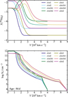 |
Fig. 1 Ejecta properties for our 1D CMFGEN model set. Top: profile of the undecayed 56Ni vs. velocity. The bump in the 56Ni abundance at higher velocities for models labeled with a b1/2 suffix does not appear in the other models, in which there is only a central concentration of 56Ni. Bottom: Profile of the electron density vs. velocity at 84 days after explosion. |
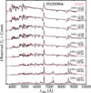 |
Fig. 2 Spectral comparison between model elnil and the observations of SN 2008bk after correction for redshift and reddening (Lisakov et al. 2017). Epochs with a star symbol correspond to data from Leonard et al. (2012a) and the others are from Pignata (2013). |
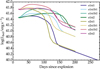 |
Fig. 3 Model light curves for our set of 1D CMFGEN simulations. |
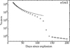 |
Fig. 4 Evolution of the total ejecta electron-scattering optical depth for model e1ni1. The two dashed curves show the expected 1/t2 evolution for an ejecta with a constant ionization. |
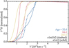 |
Fig. 5 Illustration of the comoving-frame bolometric flux H (scaled by V2 and normalized) vs. velocity for models e1ni1 (solid) and e1ni1b2 (dashed) at three epochs covering the early photospheric phase (SN age of 32 days; blue), the recombination epoch (84 days; red), and the nebular phase (200 days; yellow). |
2.2 Axially symmetric calculations with LONG_POL
The 1D CMFGEN models presented in the previous section were mapped onto 2D axially symmetric ejecta (i.e., meridional slices) following the same procedure (including grid setup, radial and angular resolution, etc.) as described for the modeling of type II-P SN 2012aw in Sect. 3.2.3 of Dessart et al. (2021b). Because the low-energy low-56Ni mass model e1ni1 is suitable for SN 2008bk (see the previous section, Fig. 2, and Lisakov et al. 2017), this model represents most of the 3D ejecta volume in our setup, while the source of the asymmetry represented by one of the other seven models occupies a small solid angle, chosen in all cases here to lie within ßc ≈ 28.13° of the symmetry axis. Specifically, we used model e1ni1 to cover polar angles between 33.75° and 90° and one of the other seven models to cover between zero and 22.50°. Linear interpolation between the two models was used to define the properties of the 2D ejecta between 22.50 and 33.75°. The quantities from the 1D CMFGEN simulations that are mapped onto the 2D ejecta are the electron density and the total opacity and emissivity at all depths and wavelengths. Top-bottom mirror symmetry is adopted so that our 2D axially symmetric structures are approximately similar to oblate or prolate ellipsoids. The left panel of Fig. 6 illustrates the evolution of the 2D contour of the location of the electron-scattering photosphere (as given by an integration along radial ejecta-centered rays) from 32 until 200 days after explosion for the 2D model e1ni1b2/e1ni1.
For our 2D ejecta models, we adopted prolate configurations with a higher kinetic energy or higher 56Ni mass in the polar direction. These configurations capture some of the features seen in 3D explosion simulations (e.g., 56Ni fingers extending into the outer ejecta, etc.; Gabler et al. 2021). In our 2D geometry, an oblate configuration for the higher-energy or 56Ni-rich material would instead correspond to a structure with a full 2π lateral coherence, as in a disk or a torus, which seems more contrived.
As nature produces a much greater variety of ejecta configurations, our choice of eight models covers only a small fraction of the existing diversity. Despite this limitation, the present mul-tiepoch polarization calculations are the first of their kind. Our choice of varying the explosion energy and the 56Ni mass treats two of the most fundamental parameters known to vary among type II-P SNe (see, e.g., Pejcha & Prieto 2015). A varying progenitor mass is unlikely to be a major factor because most type II-P SN progenitors die with a comparable H-rich envelope mass (Dessart & Hillier 2019). The influence of the opening angle, top-bottom symmetry, or explosion energy on the polarization were already explored at photospheric epochs in Dessart et al. (2021b) and at nebular epochs in Dessart et al. (2021a).
The present study is a conceptual and controlled experiment that aims to delineate the diversity of continuum polarization that may arise from the documented initial conditions. Future work will be devoted to using physically consistent 3D explosion models as initial conditions, but we caution that such simulations have their own limitations, and few have ever been evolved past a few seconds after core collapse.
Throughout this work, we also used the shape factor γ(r) to characterize the magnitude of the asymmetry. We used the modified version of the shape factor introduced by Brown & McLean (1977), such that the integral over space was performed outward from the radius r rather than over the full ejecta. Our shape factor γ(r) is thus defined as
 (1)
(1)
where Ne(r,μ) is the free-electron density at (r,μ) (μ is the cosine of the polar angle β). Spherical symmetry corresponds to γ(r) = 1/3, with a prolate (oblate) configuration corresponding to values between one-third and one (one-third and zero). A value of one corresponds to a polar line, and zero corresponds to an equatorial disk.
The shape factor was originally introduced by Brown & McLean (1977) to quantify the continuum linear polarization from an asymmetric distribution of free electrons around a point source under optically thin conditions. In our SN models, optically thin conditions are only met in the nebular phase, that is, at times greater than 130–190 days depending on the model (Fig. 3). As discussed in Appendices C and E of Dessart et al. (2021a), truly optically thin conditions in the context of polarization tend to occur even later, when the total opticall depth of the ejecta has dropped to about 0.1 or lower. At values higher than this, optical depth effects continue to operate and can quench the polarization. Optically thick regions play a subdominant role for the shape factors. In the right panel of Fig. 6 and analogs, the region beyond the photosphere (indicated by the black line) is therefore most relevant for the interpretation of the continuum polarization.
The total 56Ni mass or kinetic energy in our set of 2D axially symmetric ejecta models is equal to the 56Ni mass of the polar model weighted by (1-cos βc) and the model used for other latitudes (i.e., always model e1ni1) weighted by cos βc. Hence, our set of 2D models cover ejecta kinetic energies between 2.0 and 2.2 × 1050 erg and 56Ni masses between 0.011 and 0.015 M⊙.
The post-processing of 1D CMFGEN models with the 2D LONG_POL code is not fully consistent because the level populations at different ejecta velocities and latitudes in the 2D model are held fixed during the 2D computation with LONG_POL. The asset of LONG_POL is that it computes the 2D radiation field for the imposed 2D distribution of opacities and emissivities within the 2D ejecta, and in particular, the 2D distribution of free electrons.
In this work, we focus exclusively on continuum polarization and selected the spectral region from 6900 to 7200 Å. The results are to be compared with spectropolarimetric observations, which dominate the observational literature on SN polarization studies. They are not to be used for comparison with broadband polarimetric observations. The region from 6900 to 7200 Å is commonly used in the observational literature. In practice, LONG_POL computes the polarization throughout the optical range and explicitly accounts for the influence of line and continuum processes (see, e.g., Dessart et al. 2021b). The region between 6900 and 7200 Å is relatively line free and is therefore at all times weakly affected by metal-line blanketing (see Fig. 2). A broadening of this range from 6900 to 8200 Å (as used, e.g., by Leonard et al. 2006) yields better statistics, but this range then covers the [Ca II] λλ 7291, 7323, for example, which is strong at nebular times. We tested with each choice and found that it introduces a modest quantitative offset in the continuum polarization versus time (see Fig. B.3). Furthermore, the scattered Hα line flux could be redshifted by twice the maximum velocity of about 5000 km s−1 in the present models at most, which leads to a redshifted flux from Hα out to a maximum wavelength of about 6800 Å. Hence, the scattered Hα photons cannot affect the measured polarization beyond 6900 Å.
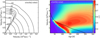 |
Fig. 6 Illustration of the electron-scattering photosphere and shape factor. Left: evolving morphology of the electron-scattering photosphere (obtained through a radial integration of the electron-scattering optical depth) in the 2D axisymmetric model e1ni1b2/e1ni1. The symmetry axis lies in the vertical direction. Only one octant is shown since our 2D simulations adopt mirror symmetry with respect to the equatorial plane. Right: corresponding evolution of the shape factor γ(r), shown as a color map, between 32 and 300 days and as function of velocity (because of homologous expansion, the radius is equal to the velocity multiplied by the SN age. Radius and velocity are therefore analogous quantities). Spherical symmetry corresponds to γ(r) = 1/3. The black line shows the representative angle-averaged location of the photosphere at each epoch. |
3 Results for a representative 2D model
Figure 7 shows results from LONG_POL for the evolution of the V-band magnitude6 and the continuum polarization from 20 to 300 days after explosion and for different viewing angles for model e1ni1b2/e1ni17 (corresponding to the 2D ejecta shown in Fig. 6). For different viewing angles, the V-band light curve lies between (and typically well away from) that of the 1D model e1ni1 (lower black curve) and that of 1D model e1ni1b2 (upper black curve). For a pole-on view, the radial extent of the electron-scattering photosphere, which is essentially at the H-recombination temperature, is unchanged relative to model e1ni1, so that a distant observer records essentially the same brightness. For an equator-on view, the radial extent of the electron-scattering photosphere is greater along the pole, increasing the size of the radiating surface relative to that seen from the pole-on view. For example, at 84 days, the photospheric radius is larger by 60% along the pole, and the equator-on view of the radiating surface is larger by about 50%, corresponding to an offset of 0.5 mag. This contrast in the size of the radiating surface with viewing angle causes the bump in V-band brightness in the second half of the photospheric phase for viewing angles closer to 90°. This bump also arises because in our low-energy model, the plateau brightness (in the absence of 56Ni) is quite low, and therefore, a high 56Ni mass as employed in model e1ni1b2 can significantly impact the otherwise faint plateau brightness. In a standard explosion model, this photometric boost from 56Ni decay heating would have had a weaker impact because low-energy explosions produce less 56Ni.
Model e1ni1b2/e1ni1 has more 56Ni than model e1ni1, but less than model e1ni1b2, that is, the ejecta transition to the nebular phase at a time intermediate (i.e., about 160 days and about the same for all viewing angles) between the times obtained for these two 1D models. The late-time brightness is systematically greater for lower latitudes with a 0.35 mag offset between a poleon and an equator-on view. The persisting dependence of the luminosity on the viewing angle is surprising at nebular times and suggests that optical depth effects still persist. There would be no photometric variation with viewing angle if the optical depth were zero, but in this model, τes is 0.48 in the pole and 0.25 in the equator direction. There is clearly residual scattering within the ejecta because LONG_POL also predicts a nonzero polarization signal, with a strong dependence on viewing angle. This issue arises because the term “optically thin” is ambiguous. While it applies for any configuration with an optical depth lower than two-thirds, ejecta with an optical depth of 0.1 or 0.001 differ from the point of view of radiative transfer.
The continuum polarization for model e1ni1b2/e1ni1 is initially zero, but rises and forms a bump at 80 days after explosion, essentially peaking at the same time as the bump seen in V-band magnitude8. The polarization at that time is maximum for mid-latitudes, which indicates that there are optical depth effects (for an optically thin configuration, the polarization would be maximum for a 90° inclination or viewing angle). The polarization then drops to a minimum at 120 days before it rises again. For most viewing angles, the maximum polarization is reached at the onset of the nebular phase, which is defined by the time when the model luminosity falls on the 56Co decay tail phase. However, for low latitudes, the continuum polarization rises until about 200days, reaching a maximum of ~1.8% for an equatoron view. The rate at which the continuum polarization decreases at late times is much slower than 1/t2. For high latitudes, the continuum polarization stays nearly constant, while at low latitudes, the decrease is close to This behavior arises for a variety of reasons. First, the ejecta optical depth is not far from unity, and therefore, the conditions are not strictly optically thin, as assumed in Brown & McLean (1977). This issue in the context of SN polarization is well known (see, e.g., Hoflich 1991; Dessart & Hillier 2011b; Dessart et al. 2021a). The ionization is not constant, but the ejecta recombination (i.e., the rate of change of the ejecta ionization) at nebular times is very slow, so that this probably plays a weak role here (see Fig. 4). The extended emission from the ejecta is more important, so that both emission and scattering occur in the same volume, in contrast with the point-source approximation assumed in Brown & McLean (1977).
In this 2D model, the continuum polarization Qcont does not change sign during the whole evolution (top right panel in Fig. B.4). It stays negative at all times and for all viewing angles. With our sign convention (see Appendix A), this indicates that the electric vector is perpendicular to the symmetry axis, as expected for the prolate 2D ejecta configuration of model e1ni1b2/e1ni1.
Further insight can be gained by inspecting the shape factor for model e1ni1b2/e1ni1 (right panel of Fig. 6). The 56Ni blob in the polar direction boosts the electron density around 2000 km s−1 (compare the curves for models e1ni1b2 and e1ni1 in Fig. 1). This leads to an asphericity of the free-electron density as well as of the electron-scattering photosphere (as given by a radial integration of the electron-scattering optical depth) after about 40 days. The shape factor γ(r) exhibits a relatively narrow peak with a maximum at the photosphere at about 80 days, which is the time of the first polarization maximum; γ(r) already reaches 0.83 at an age of 63 days, but γ(r) is relatively low above the photosphere. However, at late times, γ(r) stays high at the photosphere and is also high (i.e., about 0.7) throughout the envelope (i.e., > 1000 km s−1), with a maximum around 200 days. These variations approximately reflect the evolution of the continuum polarization shown in Fig. 7. The analogy is only approximate because of optical depth effects, which are strong during the photospheric phase and also persist until late times.
Finally, the shape factor integrated all the way to the ejecta base is much closer to one-third. The inner ejecta in model e1ni1b2/e1bni1 is nearly spherical, and because the electron density is much higher in these layers, it dominates in the integrals of Eq. (1). The polarization signature, including the jump at the onset of the tail phase, is thus clearly not tied to the asymmetry of the core, which is weak, but to the asymmetry of the outer H-rich ejecta layers, even though the electron density is weaker in these regions. This confirms the previous findings of Dessart & Hillier (2011b) and Dessart et al. (2021b).
After discussing the results for a representative case in detail, we discuss the results for the rest of the sample of 2D models calculated with LONG_POL in the next section. The contours illustrating the morphology of the 2D electron-scattering photospheres are plotted in Fig. B.2.
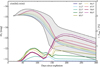 |
Fig. 7 Results for the V-band light curve and the evolution of the continuum polarization for the 2D model e1ni1b2/e1ni1. We show the evolution of the V-band magnitudes (thin lines; y-axis at the left) and continuum polarization (thick line; y-axis at the right) from 20 to 300 days. The 2D model has the properties of the 1D model e1ni1b2 for polar angles within about 28° of the axis and those of the 1D model e1ni1 elsewhere. The different colors refer to different viewing angles relative to the symmetry axis, covering from 0° (pole-on) to 90° (edge-on; see the legend in the top right corner). The gray area is bounded by the CMFGEN light curves computed for 1D models e1ni1 (bottom black curve) and e1ni1b2 (top black curve). The continuum polarization corresponds to polarization in the relatively line-free region between 6900 and 7200 Å. LONG_POL finds a null polarization at all epochs for a zero-degree inclination, as expected. |
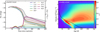 |
Fig. 8 Same as Figs. 7 and 6 (right panel), but showing the results for model e1ni1b1/e1ni1. See text for discussion. |
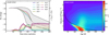 |
Fig. 9 Same as Figs. 7 and 6 (right panel), but showing the results for model e1ni2/e1ni1. See text for discussion. |
4 The evolutionary diversity of continuum polarization
Figure 8 is an analog of Fig. 7, but for model e1ni1b1/e1ni1. This 2D model exhibits qualitatively similar but quantitatively different results from those for model e1ni1b2/e1ni1 because of the slight differences in ejecta properties. The 56Ni blob at high velocity originally contains less 56Ni than model e1ni1b2, which means that the boost to the electron density is weaker (Fig. 1) and the shape factor is shifted to lower values closer to one-third (right panel of Fig. 8). The V-band bump during the photospheric phase is weaker, and so is the associated bump in continuum polarization. Optical depth effects are weaker at the end of the photospheric phase, and the continuum polarization rises sharply for inclinations at low latitudes. The decrease during the nebular phase is also steeper. The polarization curve for the viewing angle 56.2° agrees roughly with that observed for SN 2004dj (Leonard et al. 2006), but maybe accidentally, this inclination is comparable to that inferred by Chugai (2006) for SN 2004dj.
Figure 9 shows the results for the 2D model e1ni2/e1ni1. In model e1ni2, the enhanced 56Ni mass is limited to the inner ejecta (Fig. 1), which causes an increase in the radius of the electron-scattering photosphere near the end of the photospheric phase (see the top right panel of Fig. B.2). The V-band light curve is essentially independent of the viewing angle, except near the end of the photospheric phase around 150 days. The shape factor in the H-rich outer layers of the ejecta is systematically smaller than in models e1ni1b1/e1ni1 or e1ni1b2/e1ni1, and the maximum polarization never exceeds 1%. This indicates that an asymmetry confined to the inner ejecta produces a lower maximum continuum polarization than configurations where the asymmetry resides within the faster-moving H-rich ejecta (models e1ni1b2/e1ni1 or e1ni1b1/e1ni1; see Figs. 7–8).
Optical depth effects are important in at least two ways. First, there is a strong viewing-angle dependence of the continuum polarization, as can be seen by the opposite behavior of the polarization from 100 to 180 days for low and high latitudes in Fig. 9. This is caused by a sign flip for certain directions, as illustrated by the < −Qcont > evolution shown in the third panel from top in Fig. B.4. Because the configuration is optically thick, the residual polarization is influenced by both the asymmetric distribution of scatterers and the flux on the plane of the sky. Their distribution on the plane of the sky is opposite (i.e., when one appears oblate, the other appears prolate) and cancellation effects are significant. Second, the continuum polarization stays constant during the nebular phase for all viewing angles. This feature arises because the innermost ejecta regions along the pole, originally rich in 56Ni, stay hotter, more ionized, and optically thick until late times (the top right panel of Fig. B.2 indicates that the total radial electron-scattering optical depth along the poles is still greater than two-thirds at 220 days). This polarization evolution is reminiscent of that observed in SN 2008bk (Leonard et al. 2012a).
The remaining 2D configurations in our sample involve a combination of model e1ni1 with higher-energy explosions. Figure 10 shows the results for the 2D model e2ni1/e1ni1. Model e2ni1 has more mass at high velocity and less mass at low velocity than model e1ni1, so that the 2D model e2ni1/e1ni1 evolves from a prolate morphology up until 110 days to an oblate morphology thereafter (see the middle left panel of Fig. B.2). The higher explosion energy along the poles yields an enhanced brightness during the photospheric phase for viewing angles along low latitudes. The light curve is the same for all angles at late times and comparable to that of model e1ni1. The continuum polarization is nonzero throughout the photospheric phase because of the enhanced density along the poles, which causes the shape factor to reach a maximum value of 0.9 at 6000 km s−1. Because the photosphere recedes faster along the pole, the asymmetry of the 2D photosphere is continuously reduced as time passes, until it essentially becomeas spherical at 110 days. The radial variation in the optical depth is very different both above and below the photosphere for polar and equatorial directions, as illustrated by the shape factor (right panel of Fig. 10), which drops below one-third around 110days at the photosphere; at both early and late times, the shape factor is always greater than one-third beyond 1000 km s−1. The peak of polarization occurs at 110 days and reaches 1.9% for an equator-on view, even though at this time, the 2D photosphere is spherical. The ejecta regions above this spherical photosphere have a γ(r) of 0.4–0.5 and are the cause of the residual polarization. The shape of the photosphere is therefore not a reliable diagnostic for an interpretation of the polarization. When all directions become optically thin, the polarization drops abruptly and follows a slow decrease past 150 days. This well-defined narrow maximum in continuum polarization at the onset of the tail phase is qualitatively reminiscent of what was observed in SN 2008bk.
Figures 11 and 12 show the results for models e2ni1b1/e1ni1 and e2ni1b2/e1ni1, which are analogous. Because the higher-energy explosion model also has more 56Ni than model e1ni1, the 2D ejecta retain a prolate morphology at all epochs. The higher 56Ni mass boosts the ionization of the higher-energy model and compensates for the faster expansion. Models e2ni1b1 and e2ni1b2 therefore stay optically thick for longer than model e1ni1 (Fig. B.2). This is indirectly seen in the evolution of the V-band light curve. Compared to model e2ni1/e1ni1, the presence of 56Ni at high velocity maintains the shape factor near a value of 0.9 throughout the H-rich ejecta layers at >130 days. In model e2ni1b1/e1ni1, a remarkable peak polarization of 4% is reached at 130 days, followed by a rapid decrease close to the expected 1/t2 dependence. In model e2ni1b1/e1ni1, the peak is smaller at 2.7%, which is still very high, and the decrease at nebular times is slower, most likely because of the residual optical depth of the ejecta. In both models, the polarization is still about 1% for equator-on views at 300 days, which is comparable to the polarization maximum reached for a short time during the photospheric phase.
Figure 13 shows the results for the 2D ejecta model e2ni2/e1ni1. Model e2ni2 has greater kinetic energy and 56Ni mass than model e1ni1, but the Ni enhanced abundance is confined to the inner ejecta layers. While this configuration is similar to the 2D models e2ni1b1/e1ni1 and e2ni1b2/e1ni1, the continuum polarization now exhibits a plateau (roughly independent of viewing angle) during the photospheric phase and a dip near the end of the photospheric phase, followed by a sharp rise to a maximum of 1.5% for an equator-on view at the onset of the nebular phase. Unlike for models e2ni1b1/e1ni1 and e2ni1b2/e1ni1, the polarization is no longer sharply peaked.
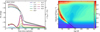 |
Fig. 10 Same as Figs. 7 and 6 (right panel), but showing the results for model e2ni1/e1ni1. See text for discussion. |
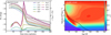 |
Fig. 11 Same as Figs. 7 and 6 (right panel), but showing the results for model e2ni1b1/e1ni1. See text for discussion. |
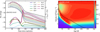 |
Fig. 12 Same as Figs. 7 and 6 (right panel), but showing the results for model e2ni1b2/e1ni1. See text for discussion. |
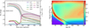 |
Fig. 13 Same as Figs. 7 and 6 (right panel), but showing the results for model e2ni2/e1ni1. See text for discussion. |
5 Conclusion
We have presented radiative-transfer calculations for axisymmetric type II SN ejecta with the aim of mapping the possible landscape of continuum polarization at photospheric and nebular epochs. Our calculations were based on 1D radiation-hydrodynamics and 1D radiative-transfer calculations of red supergiant star explosions, and the 2D polarized radiative transfer was based on crafted 2D axisymmetric ejecta obtained by the mapping in latitude of different 1D models. Using one reference model (compatible with the observed properties of SN 2008bk, Lisakov et al. 2017) for the bulk of the ejecta volume, we broke spherical symmetry by placing a distinct model in a cone along the symmetry axis. This additional model either had a higher kinetic energy or a different 56Ni mass and distribution, or both.
Despite our limited set of simulations, our models show a broad diversity in continuum polarization at a given postexplosion epoch and in the evolution of that polarization with time. The continuum polarization is generally highest at the onset of the nebular phase, as obtained previously in similar calculations (Dessart & Hillier 2011b; Dessart et al. 2021b). As discussed in those works, this rise at the onset of the nebular phase results not from the unveiling of the asymmetric metal-rich inner ejecta, but from the transition to a single-scattering regime in which polarization cancellation is reduced. The bulk of the asymmetry causing this high polarization in type II SN models is located in the extended H-rich ejecta, while the bulk of the radiation emanates from the 56Ni-rich inner ejecta. Absorption, scattering, and emission all occur over extended regions of space, which complicates the interpretation of the polarization signatures. The maximum continuum polarization reaches several percent in models with a twice higher explosion energy and enhanced 56Ni mass along the poles. The observational absence of these high values in standard core-collapse SNe suggests a moderate large-scale asymmetry. Extreme asymmetry in the form of jet explosions, for example, appear to be excluded.
High 0.5–1% polarization at early times in the photospheric phase may be produced by an asymmetric explosion (e.g., all variants based on model e2, whose kinetic energy is twice that of the reference model e1), largely regardless of the 56Ni distribution, but instead caused by the asymmetric density distribution. High polarization at early times is typically not observed in type II SNe, suggesting a modest explosion asymmetry on large scales. SN 2013ej, and more recently, SN 2021yja, are exceptions (Leonard et al. 2015; Mauerhan et al. 2017; Nagao et al. 2021; Vasylyev et al. 2023).
In contrast to observations, our simulations tend to exhibit a polarization dip at the end of the photospheric phase, just before the sudden rise to maximum. During the dip, the polarization may also flip sign, corresponding to a 90 deg change in polarization angle. This behavior likely arises from the competition between the asymmetry of the distribution of free electrons and of the flux. Enhanced scattering occurs in regions of higher optical depth, while the bulk of the flux tends to escape through regions of lower optical depth. In general, the two distributions are opposite (i.e., when the former is prolate, the latter is oblate, and vice versa). This feature may be exacerbated by our idealized 2D setup. In nature, the inner ejecta of type II SNe may be asymmetric mostly on small scales in the sense that any large-scale asymmetry may be destroyed by the numerous fluid instabilities taking place during and after the explosion. For example, the 56Ni bubble effect acting over weeks may eventually completely destroy any clean inner-ejecta asymmetry present immediately after the explosion (e.g., one minute after core bounce).
Optical depth effects are also found to persist until very late times, even in the nebular phase. This not only affects the SN brightness as seen by a distant observer from different viewing angles, but it also leads to a peculiar evolution of the continuum polarization. For example, it often deviates from a 1 /t2 fall-off, or it may even rise and peak with a delay during the nebular phase. Although clearly limited by the parameter space we explored, the plateaus in nebular-phase continuum polarization are obtained exclusively in models with enhanced inner-56Ni (i.e., models e1[2]ni2/e1ni1). The presence of isolated 56Ni blobs may also induce peculiar evolution patterns for the continuum polarization because they may locally maintain a high ionization and optically thick conditions when the rest of the ejecta is optically thin. These ionization shifts are likely strong in type II SNe because the roughly 100 days long plateau phase is fundamentally tied to recombination: Without recombination, the photospheric phase of type II SNe would last for about two years.
The late-time evolution may also be affected by our assumption of a smooth ejecta. Clumping would hasten the recombination of the ejecta (even during the photospheric phase; Dessart et al. 2018) and might hasten the drop of the continuum polarization during the nebular phase. At these times, a better treatment of chemical mixing is also warranted (Jerkstrand et al. 2012; Dessart & Hillier 2020), so that our models are not as robust as we might desire, but the standard boxcar mixing was applied here, as in the similar CMFGEN models produced for SN 2008bk by Lisakov et al. (2017), in order to keep the computational costs reasonable. Future work should be based on ejecta obtained with multi-D explosion simulations (either 2D ejecta or 3D ejecta exhibiting a dominant symmetry axis) in order to improve the physical consistency and realism of our polarization calculations.
Acknowledgements
D.C.L. acknowledges support from NSF grants AST-1009571, AST-1210311, and AST-2010001, under which part of this research was carried out. D.J.H. thanks NASA for partial support through the astrophys-ical theory grant 80NSSC20K0524. This work was granted access to the HPC resources of CINES under the allocation 2020 - A0090410554 and of TGCC under the allocation 2021 – A0110410554 made by GENCI, France. This research has made use of NASA’s Astrophysics Data System Bibliographic Services.
Appendix A Polarized radiative transfer with LONG_POL
For completeness, we summarize the nomenclature and sign conventions adopted in LONG_POL and also presented in Dessart & Hillier (2011b). We assumed that the polarization is produced by electron scattering. The scattering of electromagnetic radiation by electrons is described by the dipole or Rayleighscattering phase matrix. To describe the observed model polarization, we adopted the Stokes parameters I, Q, U, and V (Chandrasekhar 1960). We study electron scattering, and therefore, the polarization is linear and the V Stokes parameter is identically zero. For clarity, JQ and JU refer to the polarization of the specific intensity, and FQ and FU refer to the polarization of the observed flux.
For consistency with the earlier work of Hillier (1994, 1996), we chose a right-handed set of unit vectors (ζX, ζY, ζW). Without loss of generality, the axisymmetric source is centered at the origin of the coordinate system with its symmetry axis lying along ζW, ζY is in the plane of the sky, and the observer is located in the XW plane.
We took FQ to be positive when the polarization is parallel to the symmetry axis (or more correctly, parallel to the projection of the symmetry axis on the sky), and negative when it is perpendicular to it. With our choice of coordinate system, and because the SN ejecta are left-right symmetric about the XW plane, FU is zero by construction. This must be the case because symmetry requires that the polarization can only be parallel or perpendicular to the symmetry axis. For a spherical source, FQ is also identically zero.
I(ρ,δ), IQ(ρ,δ) and JU(ρ,δ) refer to the observed intensities on the plane of the sky. JQ is positive when the polarization is parallel to the radius vector and negative when it is perpendicular. In the plane of the sky, we define a set of polar coordinates (ρ, δ) with the angle δ measured counterclockwise from ζY. The polar coordinate, ρ, can also be thought of as the impact parameter of an observer’s ray. We also used the axes defined by the polar coordinate system to describe the polarization. FI is obtained from J(ρ,δ) using
 (A.1)
(A.1)
where dA = ρdδdρ. Since ζρ is rotated by an angle δ counterclockwise from ζY, FQ is given by
![Mathematical equation: ${F_Q} = {{ - 2} \over {{d^2}}}\mathop \smallint \nolimits^ _0^{{\rho _{\max }}}\mathop \smallint \nolimits^ _{ - \pi /2}^{\pi /2}\left[ {{I_Q}(\rho ,\delta )\cos \,2\delta + {I_U}(\rho ,\delta )\sin \,2\delta } \right]\,dA.$](/articles/aa/full_html/2024/04/aa47808-23/aa47808-23-eq3.png) (A.2)
(A.2)
In a spherical system, JQ is independent of δ, and IU is identically zero.
In this study, we focus on the polarization in the relatively line-free region bounded by 6900 and 7200 Å and we refer to this as continuum polarization. In practice, we quote average values over that spectral region. We either discuss the percentage continuum polarization < Pcont > defined as 100|FQ /FI| or < Qcont > defined as 100FQ/FI.
Appendix B Additional illustrations
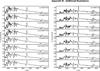 |
Fig. B.1 Spectral comparison between 1D CMFGEN models at about 20 (left) and 84 d (right) after explosion. |
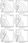 |
Fig. B.2 Same as Fig. 6 for model e1ni1b2/e1ni1, but showing the evolving morphology of the electron-scattering photosphere for the rest of the 2D model set. |
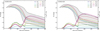 |
Fig. B.3 Influence of the spectral range used to compute the average continuum polarization. In the left panel, the range covers from 6900 to 7200 Å and in the right panel, the range covers from 6900 to 8200 Å. |
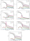 |
Fig. B.4 Same as Fig. 7, but showing the quantity < −Qcont > (averaged over the spectral region extending from 6900 until 7200 Å), which reveals any potential polarization sign flip (unlike Pcont). In the nomenclature of Dessart et al. (2021b), this quantity is defined as −100 FQ/FI (see Appendix A). We show the negative of Qcont so that most of the polarization values are positive. With our sign convention, a negative FQ corresponds to an electric vector perpendicular to the symmetry axis. |
References
- Appenzeller, I., Fricke, K., Fürtig, W., et al. 1998, The Messenger, 94, 1 [NASA ADS] [Google Scholar]
- Bollig, R., Yadav, N., Kresse, D., et al. 2021, ApJ, 915, 28 [NASA ADS] [CrossRef] [Google Scholar]
- Brown, J. C., & McLean, I. S. 1977, A&A, 57, 141 [NASA ADS] [Google Scholar]
- Chandrasekhar, S. 1960, Radiative Transfer (New York: Dover) [Google Scholar]
- Chornock, R., Filippenko, A. V., Li, W., & Silverman, J. M. 2010, ApJ, 713, 1363 [Google Scholar]
- Chornock, R., Filippenko, A. V., Li, W., et al. 2011, ApJ, 739, 41 [NASA ADS] [CrossRef] [Google Scholar]
- Chugai, N. N. 1992, Sov. Astron. Lett., 18, 168 [Google Scholar]
- Chugai, N. N. 2006, Astron. Lett., 32, 739 [NASA ADS] [CrossRef] [Google Scholar]
- Cropper, M., Bailey, J., McCowage, J., et al. 1988, MNRAS, 231, 695 [NASA ADS] [CrossRef] [Google Scholar]
- Dessart, L., & Hillier, D. J. 2008, MNRAS, 383, 57 [Google Scholar]
- Dessart, L., & Hillier, D. J. 2011a, MNRAS, 410, 1739 [NASA ADS] [Google Scholar]
- Dessart, L., & Hillier, D. J. 2011b, MNRAS, 415, 3497 [Google Scholar]
- Dessart, L., & Hillier, D. J. 2019, A&A, 625, A9 [NASA ADS] [CrossRef] [EDP Sciences] [Google Scholar]
- Dessart, L., & Hillier, D. J. 2020, A&A, 643, L13 [NASA ADS] [CrossRef] [EDP Sciences] [Google Scholar]
- Dessart, L., Livne, E., & Waldman, R. 2010a, MNRAS, 408, 827 [NASA ADS] [CrossRef] [Google Scholar]
- Dessart, L., Livne, E., & Waldman, R. 2010b, MNRAS, 405, 2113 [NASA ADS] [Google Scholar]
- Dessart, L., Hillier, D. J., Li, C., & Woosley, S. 2012, MNRAS, 424, 2139 [NASA ADS] [CrossRef] [Google Scholar]
- Dessart, L., Hillier, D. J., Waldman, R., & Livne, E. 2013, MNRAS, 433, 1745 [NASA ADS] [CrossRef] [Google Scholar]
- Dessart, L., Hillier, D. J., & Wilk, K. D. 2018, A&A, 619, A30 [NASA ADS] [CrossRef] [EDP Sciences] [Google Scholar]
- Dessart, L., Hillier, D. J., & Leonard, D. C. 2021a, A&A, 651, A10 [NASA ADS] [CrossRef] [EDP Sciences] [Google Scholar]
- Dessart, L., Leonard, D. C., Hillier, D. J., & Pignata, G. 2021b, A&A, 651, A19 [NASA ADS] [CrossRef] [EDP Sciences] [Google Scholar]
- Gabler, M., Wongwathanarat, A., & Janka, H.-T. 2021, MNRAS, 502, 3264 [CrossRef] [Google Scholar]
- Hillier, D. J. 1994, A&A, 289, 492 [NASA ADS] [Google Scholar]
- Hillier, D. J. 1996, A&A, 308, 521 [NASA ADS] [Google Scholar]
- Hillier, D. J., & Dessart, L. 2012, MNRAS, 424, 252 [CrossRef] [Google Scholar]
- Hillier, D. J., & Dessart, L. 2019, A&A, 631, A8 [NASA ADS] [CrossRef] [EDP Sciences] [Google Scholar]
- Hoflich, P. 1991, A&A, 246, 481 [NASA ADS] [Google Scholar]
- Jeffery, D. J. 1991, ApJ, 375, 264 [Google Scholar]
- Jerkstrand, A., Fransson, C., Maguire, K., et al. 2012, A&A, 546, A28 [NASA ADS] [CrossRef] [EDP Sciences] [Google Scholar]
- Leonard, D. C., Filippenko, A. V., Ardila, D. R., & Brotherton, M. S. 2001, ApJ, 553, 861 [NASA ADS] [CrossRef] [Google Scholar]
- Leonard, D. C., Filippenko, A. V., Chornock, R., & Foley, R. J. 2002, PASP, 114, 1333 [NASA ADS] [CrossRef] [Google Scholar]
- Leonard, D. C., Filippenko, A. V., Ganeshalingam, M., et al. 2006, Nature, 440, 505 [NASA ADS] [CrossRef] [Google Scholar]
- Leonard, D. C., Dessart, L., Hillier, D. J., & Pignata, G. 2012a, in American Institute of Physics Conference Series, 1429, eds. J. L. Hoffman, J. Bjorkman, & B. Whitney, 204 [NASA ADS] [Google Scholar]
- Leonard, D. C., Pignata, G., Dessart, L., et al. 2012b, ATel, 4033 [Google Scholar]
- Leonard, D. C., Dessart, L., Pignata, G., et al. 2015, IAU General Assembly, 29, 2255774 [Google Scholar]
- Leonard, D. C., Dessart, L., Hillier, D. J., et al. 2021, ApJ, 921, L35 [NASA ADS] [CrossRef] [Google Scholar]
- Li, C., Hillier, D. J., & Dessart, L. 2012, MNRAS, 426, 1671 [Google Scholar]
- Lisakov, S. M., Dessart, L., Hillier, D. J., Waldman, R., & Livne, E. 2017, MNRAS, 466, 34 [Google Scholar]
- Livne, E. 1993, ApJ, 412, 634 [Google Scholar]
- Lucy, L. B. 1991, ApJ, 383, 308 [NASA ADS] [CrossRef] [Google Scholar]
- Mauerhan, J. C., Van Dyk, S. D., Johansson, J., et al. 2017, ApJ, 834, 118 [Google Scholar]
- Maund, J. R., Wheeler, J. C., Baade, D., et al. 2009, ApJ, 705, 1139 [NASA ADS] [CrossRef] [Google Scholar]
- Mendez, M., Clocchiatti, A., Benvenuto, O. G., Feinstein, C., & Marraco, H. G. 1988, ApJ, 334, 295 [Google Scholar]
- Mezzacappa, A., Marronetti, P., Landfield, R. E., et al. 2020, Phys. Rev. D, 102, 023027 [NASA ADS] [CrossRef] [Google Scholar]
- Nagao, T., Cikota, A., Patat, F., et al. 2019, MNRAS, 489, L69 [CrossRef] [Google Scholar]
- Nagao, T., Patat, F., Taubenberger, S., et al. 2021, MNRAS, 505, 3664 [NASA ADS] [CrossRef] [Google Scholar]
- Nagao, T., Patat, F., Cikota, A., et al. 2024, A&A, 681, A11 [NASA ADS] [CrossRef] [EDP Sciences] [Google Scholar]
- O’Connor, E. P., & Couch, S. M. 2018, ApJ, 865, 81 [CrossRef] [Google Scholar]
- Paxton, B., Bildsten, L., Dotter, A., et al. 2011, ApJS, 192, 3 [Google Scholar]
- Paxton, B., Cantiello, M., Arras, P., et al. 2013, ApJS, 208, 4 [Google Scholar]
- Paxton, B., Marchant, P., Schwab, J., et al. 2015, ApJS, 220, 15 [Google Scholar]
- Paxton, B., Schwab, J., Bauer, E. B., et al. 2018, ApJS, 234, 34 [NASA ADS] [CrossRef] [Google Scholar]
- Pejcha, O., & Prieto, J. L. 2015, ApJ, 806, 225 [Google Scholar]
- Pignata, G. 2013, in Massive Stars: From alpha to Omega, 176 [Google Scholar]
- Shapiro, P. R., & Sutherland, P. G. 1982, ApJ, 263, 902 [Google Scholar]
- Swartz, D. A. 1991, ApJ, 373, 604 [NASA ADS] [CrossRef] [Google Scholar]
- Tanaka, M., Kawabata, K. S., Maeda, K., Hattori, T., & Nomoto, K. 2008, ApJ, 689, 1191 [NASA ADS] [CrossRef] [Google Scholar]
- Trammell, S. R., Hines, D. C., & Wheeler, J. C. 1993, ApJ, 414, L21 [NASA ADS] [CrossRef] [Google Scholar]
- Utrobin, V. P., & Chugai, N. N. 2005, A&A, 441, 271 [NASA ADS] [CrossRef] [EDP Sciences] [Google Scholar]
- Vartanyan, D., Coleman, M. S. B., & Burrows, A. 2022, MNRAS, 510, 4689 [NASA ADS] [CrossRef] [Google Scholar]
- Vasylyev, S. S., Yang, Y., Filippenko, A. V., et al. 2023, ApJ, 955, L37 [NASA ADS] [CrossRef] [Google Scholar]
- Wang, L., & Wheeler, J. C. 2008, ARA&A, 46, 433 [Google Scholar]
- Woosley, S. E., Heger, A., & Weaver, T. A. 2002, Rev. Mod. Phys., 74, 1015 [NASA ADS] [CrossRef] [Google Scholar]
The positive correlation between 56Ni mass and explosion energy is inferred from observations (see, e.g., Pejcha & Prieto 2015) and is theoretically understood to arise from the dependence between explosion energy, post-shock temperature, and explosive nucleosynthesis. Roughly speaking, shocked material with a temperature in excess of 5 × 10⁹ K burns to iron-group elements. If its electron fraction is close or equal to 0.5, the main isotope will be 56Ni (see, e.g., Sect. VIII of Woosley et al. 2002).
An observational study with a similar focus but different methodology was published by Nagao et al. (2024) as we completed the writing of this manuscript. The bulk of the work and analysis presented here was done two years ago.
VLT-FORS stands for Very-Large-Telescope FOcal Reducer and low dispersion Spectrograph (Appenzeller et al. 1998).
So far, spectropolarimetric observations have typically been obtained for nearby events, which for the vast majority arise from solarmetallicity environments. This choice is therefore sensible. In practice, metal-line blanketing reduces the albedo and has an adverse effect on polarization. Variations in metallicity will modulate this. However, when considering spectral regions that are relatively line free at most photospheric epochs (around 7000 Å), metallicity variations should have little impact. In the nebular phase, the continuum is weak and lines dominate, many arising from metals that were produced during the explosion (which are therefore unaffected by the original metallicity of the progenitor on the zero-age main sequence).
CMFGEN solves for the radiative transfer, but ignores the hydrodynamics. We therefore start the CMFGEN sequences when the dynamical phase is complete, which takes 10–15 days in RSG star explosions because of the slow reverse-shock that progresses inward into the metal-rich ejecta (see the discussion in Dessart & Hillier 2011a) – this is standard practice in all our simulations of type II-P SNe.
We illustrate the V-band magnitude rather than a pure continuum magnitude because the latter is not routinely observed.
The naming convention used here and for all 2D models is defined in Table 1. Specifically, the model name lists the model inserted into the polar regions within ≈ 28.13° first (here e1ni1b2), followed by the base model employed for the rest of the ejecta (here, and in all cases, e1ni1).
As discussed above for the V-band light curve, a smaller amount of 56Ni would yield a smaller polarization bump because the excess in the free-electron density would be less. See the next section and discussion for the model e1ni1b1/e1ni1. The impact of a higher explosion energy, more typical of a standard type II-P SN, on the polarization is less clear because in this case, the mass density, the ionization, and thus the free-electron density would change even without a high-velocity 56Ni blob. Results for this case were presented in Dessart et al. (2021b), however.
All Tables
Summary of radiative transfer simulations in both 1D (upper part) and 2D (lower part).
All Figures
|
Fig. 1 Ejecta properties for our 1D CMFGEN model set. Top: profile of the undecayed 56Ni vs. velocity. The bump in the 56Ni abundance at higher velocities for models labeled with a b1/2 suffix does not appear in the other models, in which there is only a central concentration of 56Ni. Bottom: Profile of the electron density vs. velocity at 84 days after explosion. |
| In the text | |
|
Fig. 2 Spectral comparison between model elnil and the observations of SN 2008bk after correction for redshift and reddening (Lisakov et al. 2017). Epochs with a star symbol correspond to data from Leonard et al. (2012a) and the others are from Pignata (2013). |
| In the text | |
|
Fig. 3 Model light curves for our set of 1D CMFGEN simulations. |
| In the text | |
|
Fig. 4 Evolution of the total ejecta electron-scattering optical depth for model e1ni1. The two dashed curves show the expected 1/t2 evolution for an ejecta with a constant ionization. |
| In the text | |
|
Fig. 5 Illustration of the comoving-frame bolometric flux H (scaled by V2 and normalized) vs. velocity for models e1ni1 (solid) and e1ni1b2 (dashed) at three epochs covering the early photospheric phase (SN age of 32 days; blue), the recombination epoch (84 days; red), and the nebular phase (200 days; yellow). |
| In the text | |
|
Fig. 6 Illustration of the electron-scattering photosphere and shape factor. Left: evolving morphology of the electron-scattering photosphere (obtained through a radial integration of the electron-scattering optical depth) in the 2D axisymmetric model e1ni1b2/e1ni1. The symmetry axis lies in the vertical direction. Only one octant is shown since our 2D simulations adopt mirror symmetry with respect to the equatorial plane. Right: corresponding evolution of the shape factor γ(r), shown as a color map, between 32 and 300 days and as function of velocity (because of homologous expansion, the radius is equal to the velocity multiplied by the SN age. Radius and velocity are therefore analogous quantities). Spherical symmetry corresponds to γ(r) = 1/3. The black line shows the representative angle-averaged location of the photosphere at each epoch. |
| In the text | |
|
Fig. 7 Results for the V-band light curve and the evolution of the continuum polarization for the 2D model e1ni1b2/e1ni1. We show the evolution of the V-band magnitudes (thin lines; y-axis at the left) and continuum polarization (thick line; y-axis at the right) from 20 to 300 days. The 2D model has the properties of the 1D model e1ni1b2 for polar angles within about 28° of the axis and those of the 1D model e1ni1 elsewhere. The different colors refer to different viewing angles relative to the symmetry axis, covering from 0° (pole-on) to 90° (edge-on; see the legend in the top right corner). The gray area is bounded by the CMFGEN light curves computed for 1D models e1ni1 (bottom black curve) and e1ni1b2 (top black curve). The continuum polarization corresponds to polarization in the relatively line-free region between 6900 and 7200 Å. LONG_POL finds a null polarization at all epochs for a zero-degree inclination, as expected. |
| In the text | |
|
Fig. 8 Same as Figs. 7 and 6 (right panel), but showing the results for model e1ni1b1/e1ni1. See text for discussion. |
| In the text | |
|
Fig. 9 Same as Figs. 7 and 6 (right panel), but showing the results for model e1ni2/e1ni1. See text for discussion. |
| In the text | |
|
Fig. 10 Same as Figs. 7 and 6 (right panel), but showing the results for model e2ni1/e1ni1. See text for discussion. |
| In the text | |
|
Fig. 11 Same as Figs. 7 and 6 (right panel), but showing the results for model e2ni1b1/e1ni1. See text for discussion. |
| In the text | |
|
Fig. 12 Same as Figs. 7 and 6 (right panel), but showing the results for model e2ni1b2/e1ni1. See text for discussion. |
| In the text | |
|
Fig. 13 Same as Figs. 7 and 6 (right panel), but showing the results for model e2ni2/e1ni1. See text for discussion. |
| In the text | |
|
Fig. B.1 Spectral comparison between 1D CMFGEN models at about 20 (left) and 84 d (right) after explosion. |
| In the text | |
|
Fig. B.2 Same as Fig. 6 for model e1ni1b2/e1ni1, but showing the evolving morphology of the electron-scattering photosphere for the rest of the 2D model set. |
| In the text | |
|
Fig. B.3 Influence of the spectral range used to compute the average continuum polarization. In the left panel, the range covers from 6900 to 7200 Å and in the right panel, the range covers from 6900 to 8200 Å. |
| In the text | |
|
Fig. B.4 Same as Fig. 7, but showing the quantity < −Qcont > (averaged over the spectral region extending from 6900 until 7200 Å), which reveals any potential polarization sign flip (unlike Pcont). In the nomenclature of Dessart et al. (2021b), this quantity is defined as −100 FQ/FI (see Appendix A). We show the negative of Qcont so that most of the polarization values are positive. With our sign convention, a negative FQ corresponds to an electric vector perpendicular to the symmetry axis. |
| In the text | |
Current usage metrics show cumulative count of Article Views (full-text article views including HTML views, PDF and ePub downloads, according to the available data) and Abstracts Views on Vision4Press platform.
Data correspond to usage on the plateform after 2015. The current usage metrics is available 48-96 hours after online publication and is updated daily on week days.
Initial download of the metrics may take a while.