| Issue |
A&A
Volume 684, April 2024
|
|
|---|---|---|
| Article Number | A115 | |
| Number of page(s) | 14 | |
| Section | Astrophysical processes | |
| DOI | https://doi.org/10.1051/0004-6361/202347692 | |
| Published online | 10 April 2024 | |
Ab initio simulations of neutron stars’ oblique electrospheres with realistic neutron star parameters
Laboratoire Univers et Théories, Observatoire de Paris, CNRS, Université PSL, Université Paris Cité, 92190 Meudon, France
e-mail: This email address is being protected from spambots. You need JavaScript enabled to view it.
Received:
10
August
2023
Accepted:
23
January
2024
Abstract
Context. Electrospheres are environments with the same origin as pulsars; a highly magnetized rotating neutron star. In pulsars, a cascade of electron-positron pair creation enriches the plasma. The plasma surrounding an electrosphere consists only of particles that have escaped from the neutron star’s surface. Electrospheres with a magnetic axis aligned with the rotation axis have been well described for decades. Models of electrospheres with an oblique magnetic axis relative to the rotation axis have resisted most theoretical investigations. Some electrospheres and pulsars have been simulated using particle-in-cell codes, but the numerical constraints did not allow the use of realistic neutron star parameters.
Aims. We aimed to develop a numerical simulation code optimized for understanding the physics of electrospheres and pulsars, with realistic neutron star parameters. As a first step, presented in this paper, we focused on the simulation of oblique electrospheres with realistic physical parameters.
Methods. A specific code was developed for the computation of stationary solutions. The resolution of Maxwell’s equations was based on spectral methods. Particle motions included their finite inertia. No hypothesis was made in relation to the force-free behavior of the electrospheric plasma. The numerical code is called Pulsar ARoMa (pulsar asymmetric rotating magnetosphere).
Results. Various numerical simulations were conducted using realistic neutron star parameters. We find that oblique electrospheres possess the same global structure as aligned force-free electrospheres, with two domes of electrons and a torus of positively charged particles. The domes are not centered on the magnetic axis; nor are they symmetric. Yet, the solutions do not exhibit a force-free behavior.
Conclusions. The simulations performed with the Pulsar ARoMa code require modest resources and little computing time. This code will be upgraded for more ambitious investigations into pulsar physics.
Key words: methods: numerical / stars: magnetic field / stars: neutron / pulsars: general
© The Authors 2024
 Open Access article, published by EDP Sciences, under the terms of the Creative Commons Attribution License (https://creativecommons.org/licenses/by/4.0), which permits unrestricted use, distribution, and reproduction in any medium, provided the original work is properly cited.
This article is published in open access under the Subscribe to Open model. This email address is being protected from spambots. You need JavaScript enabled to view it. to support open access publication.
1. Introduction
Since their discovery by Hewish et al. (1969), considerable progress has been made in modeling pulsars. However, considerable progress is also needed to really understand the physical mechanisms governing these highly energetic objects. In this paper, a step forward toward this goal is presented, based on the writing of a new numerical simulation code named Pulsar ARoMa (pulsar asymmetric rotating magnetosphere) that enables the fundamental equations governing the electrodynamics of pulsars to be solved, in a regime that allows the use of realistic parameters.
As soon as pulsars were recognized as manifestations of neutron stars’ (NSs’) environments, the problem could be posed physically in a very simple way as that of a magnetized, electrically conductive, rapidly rotating sphere in an initially empty medium. Generally, the magnetic field at the surface of the star is considered to be dipolar, but multipolar components are also possible. The symmetry axis of the magnetic field can make any angle with the rotation axis of the NS (oblique pulsars), but for computational ease, solutions with a dipole aligned with the rotation axis (aligned pulsars) have been given special attention.
The first step in solving the pulsar problem was the calculation of the electromagnetic field into the vacuum extending around the NS. For an oblique dipole, a previous computation by Deutsch (1955) showed that the solution is close to the dipole solution in the vicinity of the star, but extends beyond the light cylinder in the form of a wave propagating at the speed of light, whose wave front is deployed along an Archimedes spiral. This wave carries a Poynting flux that corresponds in part with the loss of rotational energy of the pulsar (Gold 1968; Pacini 1967). A vacuum solution with a multipolar magnetic field was developed more recently (Bonazzola et al. 2015; Pétri 2015). An important element of the vacuum solution is the fact that the rotating NS behaves like a unipolar inductor, generating a large-amplitude electric field at the star’s surface.
However, it has been shown in Goldreich & Julian (1969) that the surface electric field repels electrons and ions from the star’s surface and accelerates them to very high energies. As a result, the NS is embedded in a plasma, not in an empty region. Goldreich & Julian (1969) applied the concept of a unipolar inductor to NSs, assuming that the plasma near the star was rotating with it. They then developed the fundamental concept of a corotation space charge of the plasma, deduced from the divergence of the corotation electric field. Unlike most astrophysical objects, this charge density is high in the vicinity of NSs, due to their high rotation rate and magnetic field. They thus showed that there is a non-neutral, plasma-filled magnetosphere around NSs. The concept of a corotation charge cannot be applied at locations near and beyond the light cylinder, but it lays the foundation for understanding the internal boundary conditions of the pulsar, near its surface.
The electrons extracted from the NS’s surface are called primary electrons. They follow a curved trajectory, the curvature being those of the NS magnetic field lines (with a curvature radius ∼100 km). Because of the high electric fields above the surface, the primary electron can reach Lorentz factors of several million, and they emit gamma ray photons. Sturrock (1970) showed that their interaction with the magnetic field of the NS generates energetic pairs of electrons and positrons that, in turn, emit gamma rays and other pairs, and thus cause a cascade of pair creation. Pairs can also be created by gamma ray photons interacting with thermal (X-ray) photons emitted by the NS. Timokhin & Harding (2019) made an evaluation of the cascade efficiency with the help of a local (1D) semi-analytical model of the acceleration region. In highly magnetized pulsars, the efficiency of the cascades can reach a factor of a few 105 pairs created for each primary electron.
All these works highlighted important facts about pulsars, but the construction of a global picture remained to be done. Many works have been devoted to this difficult task. Since the early 2000s, most of them have been based on numerical simulations. They are reviewed in Cerutti & Beloborodov (2017). In a seminal work, Krause-Polstorff & Michel (1985) showed that a NS magnetosphere without pair creation is formed by two domes of electrons above the polar caps and of a belt of positively charged particles near the magnetic equator. This is called an electrosphere. With only one exception (McDonald & Shearer 2009), electrospheres were described only for an aligned magnetic field.
Higgins & Henriksen (1997) developed a radiation model for the high-energy emission from pulsars considering charged particle motion in the fields of a spinning, highly magnetized, and conducting sphere in a vacuum. The electromagnetic field corresponded to the Deutsch (1955) vacuum solution, and there was no pair creation. The radiation emitted by curvature emission was summed to generate light curves. The calculation was simplified analytically, but something equivalent to the electrosphere appeared.
In this paper, models of electrospheres are presented. They are based on numerical simulations. They have a few characteristics that are not met simultaneously in the literature, as far as we know. The bad news is that the models presented in this study are stationary. They do not permit analysis of the possible development of plasma instabilities. The good news is the following. The models include particles with finite inertia. The particles have real masses and real charges. There are no reduced variables, ordinary physical units can be used to characterize a set of simulation parameters, and the model includes realistic NS radii, rotation rates, and magnetic field amplitudes. The magnetic field emerging from the NS is dipolar, but this choice was simply made for the sake of simplicity. There was no a priori hypothesis about a force-free region. We supposed a zero work function for the extraction of particles from the stellar surface. A large set of models of oblique electrospheres is presented.
This step is intermediate and does not yet allow the complete pulsar dynamics to be simulated, because the version presented here does not take into account radiative phenomena and the pair creation phenomenon. It does however allow the simulation of solutions belonging to the electrosphere family that, from an astronomical point of view, can represent “dead pulsars,” beyond the death line (or death valley) of the P − Ṗ diagram (Beskin & Litvinov 2022).
The units used in the simulations are ordinary CGS units, unless stated otherwise. We frequently use the adjectives “parallel” and “perpendicular” to characterize vectors. This is relative to the direction of the local magnetic field, B. Of course, these adjectives only make sense when B ≠ 0; otherwise, we don’t use them.
2. Particle inertia and electrospheres
Before explaining the method used in our numerical simulations, we discuss the role of particle inertia in electrospheres.
A large class of electrosphere models is based on the hypothesis introduced by Krause-Polstorff & Michel (1985) of particles without inertia. If such particles encounter a finite parallel electric field, they reach a velocity, c, and talking about their Lorentz factor is meaningless. Therefore, any equilibrium involving such particles implies force-free conditions, E ⋅ B = 0, in any place containing a plasma. Non-force-free electromagnetic fields are possible only in vacuum gaps; that is, regions with no particles. There are two practical consequences regarding electrospheres. First, the dome containing electrons, and the torus containing ions or positrons, are force-free. Second, the inner boundary conditions just above the surface of the star are also force-free.
An interesting consequence of this last condition is that there is no real connection between the star and its electrosphere, and the equations describing this family of models of electrospheres show that the total electric charge of the electrosphere is a free parameter.
Smith et al. (2001) conducted numerical simulations of aligned electrospheres with particles without inertia. They showed solutions for a large range of magnetospheric global charges, as was stated by Krause-Polstorff & Michel (1985). Their solutions for typical pulsar parameters were all encompassed within the light cylinder but the authors remarked that, if there were a loss in the system, it would not lead to a replacement by particles escaping from the star.
Pétri et al. (2002) independently developed a semi-analytical theory of aligned electrospheres, starting from the same hypothesis. They reached the same conclusions. They also showed that the geometric and kinematic structure of the electrosphere is uniquely determined by the total charge of the system, and that the conditions for a cascade of electron-positron pair creations are not met (except maybe for a millisecond pulsar). A practical consequence of this last conclusion, compatible with up-to-date radio astronomical observations, is that aligned electrospheres can exist, but aligned pulsars cannot exist.
In the present study, particles have a finite inertia. They are governed by a sum of the Lorentz electromagnetic force and a reaction force caused by the radiations that they emit. Because of their inertia, particles can be accelerated by finite parallel electric fields without reaching infinite Lorentz factors. Therefore, there is no need to settle force-free conditions above the surface of the star. Hence, the electrosphere is not isolated from the star, and a self-consistent electrospheric total charge can be established. It is not an ad hoc parameter, as is the case in force-free electrospheres.
Our simulations contain force-free zones. Particles don’t necessarily find an equilibrium position within them; they can oscillate around them, sometimes, as we shall see, with a spatial amplitude that can encompass very large regions.
Philippov & Spitkovsky (2014) simulated one aligned electrosphere with a particle-in-cell (PIC) code. In order to minimize the computational expense, the simulation was run with a star that had a high rotation rate, resulting in a light cylinder distance, RLC, of only 2.6 star radii, R*. As in force-free models, the electrosphere contains a dome of positrons above each pole, and an equatorial belt of electrons. (The magnetic field axis being opposite to the rotation axis, the signs of electric charges in these two regions are exchanged.) They showed that the current flow is insufficient to appreciably modify the dipole magnetic field structure or cause pulsar spin-down. Very little was said about the global electric charge of the electrosphere, or about the mapping of the parallel electric field, so it is difficult to compare this simulation with those involving the force-free approximation.
McDonald & Shearer (2009) made the only simulations of oblique electrospheres. A PIC code was used and particles had a finite inertia. The surface of the star was initially not force-free, but they considered that the convergence toward an electrosphere solution was reached when, at the stellar surface, E ⋅ B approached a null value. Nothing is said in their paper about the particle injection process from the stellar surface into its environment, such as the particles’ energies or the flux of the injected particles. There are probably several ways of injecting particles and they probably have an influence on the properties, and even the existence, of the electrosphere.
In the present work, we don’t impose any force-free condition. We consider that, right above the surface of the star, particles can escape at high energies owing to the parallel electric field allowed in our simulations. This does not imply necessarily that a net flux of particles leaves each portion of the surface. Indeed, particles can go back toward the surface and reach it. (The same thing was possible in McDonald & Shearer 2009, but only before an equilibrium was reached.) The main difference is that the particles coming back into the star are decelerated, while the same particles living the surface are accelerated. Therefore, with a finite particle inertia, a static equilibrium can be reached through a dynamic process involving particles quitting the surface and returning back to it (not necessarily in the same place), without the necessity of a null parallel field above the stellar surface.
3. Method
3.1. General principles
The main data of a simulation consist of an electromagnetic field recorded on a 3D grid, a charge density and a current density recorded on the same 3D grid, a particle distribution recorded on a 4D phase-space grid, and a series of pseudo-particle trajectories.
A simulation consists of a series of iterations, during which all simulation data are re-evaluated. Since the complete particle trajectories are calculated during an iteration, and since we are looking for a stationary solution, not a time-dependent one, an iteration does not correspond to a time interval. It corresponds to an undefined period of time. An iteration is (ideally) a step in a process of convergence from initial conditions that are not a solution of the pulsar problem to a time-independent solution. The term “ideally” in brackets simply underlines the fact that convergence is not guaranteed.
The elements of the pseudo-particle trajectories consist of their contribution, f, to the phase-space distribution, for a position, xi, a Lorentz factor, γi, and a velocity, vi, at times, ti, elapsed since the beginning of the trajectory (t0 = 0). For practical reasons, a particle trajectory contains a maximum number, Pmax, of elements or time steps, i. In most of the simulations presented here, Pmax = 10 000.
The pseudo-particle trajectories obey the equation of motion
 (1)
(1)
where v is the pseudo-particle velocity, γ is its Lorentz factor, and q and m are its electric charge and mass, respectively. The velocity is a 3D vector. No particular assumptions are made about the value of its parallel or perpendicular component. The vectors E and B represent the local electric and magnetic fields. The pseudo electric field ER represents a counter reaction force caused by the particle radiation. More details are given in Sect. 3.4.
Generally, a particle trajectory is stopped when it quits the simulation domain, either falling onto the star (inner boundary), or when it crosses the outer boundary, at a large distance from the star. A particle represents a fraction of the particle distribution. When a pseudo-particle ends its trajectory (i = Pmax) and is still in the simulation domain, the last element of the trajectory is stored in a 4D phase-space density and becomes the starting point of a new trajectory that will be computed at the next iteration. Ideally, the phase space should have six dimensions representing the positions, x, and the momentum. Actually, the particles in the vicinity of a NS have a very high energy. Consequently, they are strong emitters of synchrotron radiation as soon as they have a finite perpendicular momentum. Therefore, the perpendicular momentum quickly tends to zero. We assume that this observation, which is true in general, is systematically true; this is why the particle is stored in a 4D phase space whose components represent the three dimensions of space, and the parallel momentum.
The positions in space, xi, occupied by the different elements of a trajectory were used to calculate the contribution of the pseudo-particle to the charge density, ρ(x), and the current density, J(x), whose values are defined on each element of the 3D grid.
The charge and current densities on the grid are the source terms of the Maxwell equations. Once a new electromagnetic field was computed onto the 3D grid, a new iteration could take place, unless we considered that the simulation code had reached a stationary solution.
The convergence toward a stationary solution is checked “visually” and through an evaluation of the total electric charge outside the star. Its variations must converge toward a constant value. Generally, when convergence is reached, the residual amplitude of the fluctuations of the total charge density of the electrosphere is on the order of one percent. In the present paper, convergence was reached after three or four iterations, and most simulations were conducted with ten or 15 iterations in order to ensure the numerical stability of the solution.
3.2. Simulation grid
The grid on which the electromagnetic field, the charge density, the current density, and the particle distributions were computed is a lattice of lines of constant spherical coordinates. The origin of coordinates is at the stellar center. The principal axis of these coordinates is the stellar rotation axis. There are Nangles, lines of equally spaced planes of fixed azimuth, ϕi, and the same number of cones of equally spaced colatitude, θi (i ∈ [1, Nangles]). This grid is appropriate for the resolution of Maxwell’s equations with the use of spherical harmonic functions. Unless stated otherwise, Nangles = 32.
The radial coordinate, r, is associated with spheres of radius rj. The sphere indexed by a number zero has a radius, r0, equal to the star’s radius, R*. The increments rj + 1 − rj are not uniform, because a high resolution (meters or centimeters) is needed above the stellar surface and a lower resolution is permitted at larger distances. The simulation grid is a sphere containing Nd domains connected to each other, each domain containing Nnodes, Gauss-Lobatto nodes defined as xj = cos(πj/Nnodes), which are appropriate with a decomposition of the electromagnetic field (for the r variable) in Chebychev polynomials (Grandclément & Novak 2009). The Nd domains do not have the same size. In most simulations of the present study, the first domain, close to the star, has a size of 10−4 × R*. After Riley et al. (2021), a star’s radius, R* = 12 km, was set. The first domain has a size of 1.2 m. The distance between the two first nodes of this domain is 1.15 cm. There are Nd = 11 domains and Nnodes = 16 nodes per domain. The size of the second domain is 12 m, then 120 m and 1.2 km, and the following domains are twice as large as the previous ones. Therefore, the total radius of the simulation domain is 1700 km = 142 R*. The simulation domain contains the light cylinder.
The particle distributions for each species, s, were also stored on a grid representing a reduced 4D phase space. The first three coordinates are the space coordinates (r, θ, ϕ); the last is the absolute value of the parallel impulsion normalized to the particle mass, U = p∥/ms = γv∥, completed by the sign, s, of p∥ relative to the radial direction (negative if the particles go in the direction of the star). In the present version of the code, the parallel impulsion cells are defined in the same way as the r cells, as a series of Ndp domains containing Nnodesp, which are Gauss-Lobatto nodes. This is actually for historical reasons, since spectral methods are not used in the end to deal with the particle impulsion, and hence this could be changed.
3.3. Electromagnetic field solution
As in Pétri (2013), we used a spectral method to solve Maxwell’s equations, where all the fields were decomposed on a basis of spherical harmonic functions of θ and ϕ, and, for each domain, on a basis of Chebychev functions of r. A description of this method is given in Grandclément & Novak (2009) and useful additions to this document are given in the appendix to Pétri (2013). The main differences with the present work are that Pétri (2013) solved a general relativistic version of Maxwell’s equations (for a given metric), whereas we only considered special relativity. In Pétri (2013), only one simulation domain for the Chebychev functions in r was used, while Nd > 1 domains were used in the present work.
3.4. Motion of pseudo particles
The equation of motion (1) was solved using a relativistic version of an algorithm that solves the motion of the guiding center (Mottez et al. 1998; Mottez 2008). The implementation of special relativity was derived from Vay (2008). This method actually provides the guiding center motion of the particle if the time step, Δt, is large compared to the particle gyrogrequency, Ωs; in other words, if ΔtΩs ≫ 1. In the reverse case, it provides the full motion of the particle. The highly inhomogeneous environment of a NS imposes a very low time step, Δt, near the stellar surface and in acceleration regions; but it would allow higher values in other regions of the electrosphere. In order to increase the computational efficiency of the simulation, the implementation of a method of computation of pseudo-particle trajectories with variable time steps was set and validated.
In the simulations presented in the following sections, because of the very high electric fields near the star’s surface where particles are emitted, we started with a time step, cΔt < 0.1 mm. At greater distances from the star, the algorithm provided a time step up to cΔt ∼ 10 m.
This algorithm, its implementation, and testing can be useful for other applications and will be presented in a future article, because their field of application goes beyond pulsars and astrophysical applications.
3.5. Radiative losses by curvature radiation
The particles were accelerated to ultra-relativistic energies and moved in a magnetized environment: radiative losses due to the acceleration are very important. In these conditions, loss associated with synchrotron emission annihilates the high-frequency motion perpendicular to the local magnetic field. Therefore, their pitch angle is zero. Synchrotron radiation losses are important only when new particles are created. But curvature radiation, caused by the curvature of the particles’ trajectories along magnetic field lines, cannot be neglected. The power loss is (in Gaussian units)
 (2)
(2)
where Cm is the curvature of their trajectory, which we equate with the curvature of local magnetic field lines. This power can be likened to the work (per time unit) of a force caused by an electric field, qvER ∼ cqER, that is anti-parallel to the particle velocity. The electric field, ER, is the one appearing in Eq. (1).
Since the magnetic field was known for each iteration, computing Cm was straightforward. But, with highly-relativistic particles, and hence large Lorentz factors, the γ4 factor in the definition of ER was the potential source of a numerical runaway instability, with γ increasing in a non-physical way. Actually, various tests proved that this numerical instability occurs occasionally in a few regions of the simulation domain situated very near to the NS surface. Therefore, we added a calculation rule for particle movement: if, during a single time step, the Lorentz factor was multiplied by a given factor (on the order of five, but this can be adjusted), the instability occurs. Then, it was considered that the inertia of the particle is of no importance (in spite of it being the cause of the numerical instability), and an asymptotic Lorentz factor, γa, was established to ensure equality between the electrical acceleration force and the radiation reaction force:
 (3)
(3)
The particle Lorentz factor was updated with this value, and the direction of motion was conserved. At the next iteration of the particle trajectory, the computation based on Eq. (1) and on ER was applied again, without necessarily resorting to Eq. (3).
In the present case, Eq. (3) provides the particle energy in particular cases where the use of Eq. (2) would lead to a numerical instability. Actually, the systematic use of Eq. (3) for the computation of the particle energy (that is not implemented here) would constitute a reasonable approximation, and was used in Higgins & Henriksen (1997).
3.6. Particle transport and charge deposition
The transport of charge and current densities by particles was treated in a specific way, taking into account the stationary nature of the solution sought, the fact that an iteration does not correspond to a specific duration, the fact that each time step in a particle trajectory may be different from the others, and the volumes of each cell in the simulation domain potentially being different from one another. A certain formalism is needed to describe the algorithm that takes all these facts into account.
Let us consider a set of particles that have been created at time, t0, or that have emerged from a boundary, and that have propagated since then in the absence of creation, destruction, or scattering between particles. The conservation of the distribution function along their trajectories implies that for any time, ti,
 (4)
(4)
For the sake of economy, we characterized the position in the phase-space with a vector, x = (r, θ, ϕ), and u = (U, s), x0 = x(t0), and xi = x(ti). Equation (4) reads simply
 (5)
(5)
where x(ti) is the trajectory of particles initially at xj and u(ti) is its momentum in the direction along the local magnetic field. The particle trajectory was computed with the solution mentioned in Sect. 3.4 and produced the transformation (x0, u0)→(xi, ui) for any time, ti > t0. We considered f to be known at time t0 at every node, j, of the phase-space grid.
The number of particles, δN = fδVδU, is constant along the trajectory, where δV is the volume in space and δVδU is the phase-space volume. Consequently (Liouville theorem), the element of phase-space volume δVδU is conserved. We note that δV(ti)δU(ti) and abbreviate δ(UV)i, the element of volume associated with these particles at time ti, and Δ(UV)i, the element of volume associated with the phase-space grid cell, Ω(ti), used in the code, which includes the position, xi, of the particles at time ti.
Let us consider the cell Ω0 = Ω(x0). The particles initially in that cell have moved into another cell, Ω(xi). The conservation of the particle number created at time t0 in the phase-space cell, Ω0, reads as ΔN = f(x0, t0)Δ(UV)0 = f(xi, ui, ti)δ(UV)i. At time t0 we considered the volume, δ(UV)0, physically occupied by the particles to be that of the cell space, Δ(UV)0. The volume, δUV(xi, ui, ti), physically occupied by the particles is not necessarily equal to the phase-space volume, Δ(UV)i, of the grid cell corresponding to the position of these particles at time ti. A set of particles, p, created at time t0 in the cell, Ω0, then contribute to the particle number in phase-space cell, Ω(xti), to an amount,
 (6)
(6)
and to the particle phase-space density,
 (7)
(7)
Either of these two quantities, ΔN or f, can be added into an array that has the same dimensions as the phase-space grid. The total phase-space density is the sum of the contribution of all the source terms, f(x0, u0, t0), associated with the phase-space grids, Ω0, for pseudo-particles arriving in the phase-space grid, Ωj:
 (8)
(8)
Actually, we placed not one but Npart particles initially in each phase-space cell, Ω0. Their positions in that cell were computed randomly with a uniform law. This was done in order to reduce the particle noise that corresponds to a finite sampling of the initial positions of the particles. The sum in Eq. (8) includes these Npart particles in each cell, Ω0.
The charge density is ρ = ∫qsf(xi, ui, ti)dui. The contribution of a trajectory to the total charge in the spatial grid element, Xi, corresponding to Ωi is
 (9)
(9)
In Eq. (10) and subsequent formulas, (xi, ui)∈Ω is replaced by (xi)∈Xi.
The contribution to the charge density is
 (10)
(10)
and the same normalization coefficients apply to the current density and, for diagnostics, to the particle density and the mean velocity (to be normalized in time by the particle density).
3.7. Three arrays that represent the particle phase-space flux
In the code, the connection between particles and charge and current densities is based on a 4D array called FFF that contains the flux of particles,
 (11)
(11)
This corresponds to the sources, ΔN0, divided by the time, Δt0, necessary to cross the cell at the start of the iteration, istep. It does not contains the effect of particle transport, and therefore is not yet the value of ΔN(xi, ui, ti). The contribution of the trajectories to the electric charge is the flux multiplied by the time step of the trajectory element, ti:
 (12)
(12)
and the contribution to the charge density is
 (13)
(13)
Because the model is stationary, we need the average values of the total charge and of the charge density:
 (14)
(14)
and the contribution to charge density is
 (15)
(15)
where T = ∑iΔti is the total duration of the trajectory.
Another array, called FFA, contains the flux of ΔN(xi, ui, ti) at the end of the iteration, istep. Up to now, FFA had been computed to test the feasibility of the computation, but not yet used. The array, FFA, will be used in the future, when we include radiative effects and pair creation processes.
During the iteration, new source terms were computed and assigned to FFB. For a particle trajectory ending in the simulation domain, the last position of this particle contributes to FFB. More details are given in Sect. 3.12. When new electron-positron pairs are created (in future studies), they will also contribute to FFB.
We made tests of radial propagation at the speed of light, with different types of injection at the inner boundary: uniform, random, and impulsive. In all cases, the simulation box was initially empty, and therefore there had to be the propagation of a front of particles. With a non-monotonic Hermite interpolation of the third order, the results were not very good: there was a lot of diffusion, a precursor that goes much faster than light, and a non-uniform repartition of the particles, even when they were injected at a constant rate. It was therefore decided to instead use a rough but simple and robust method of interpolation of the zeroth order, whereby all the particle weight (mass, charge) was assigned to a single phase-space cell. Testing with injection at a constant rate enabled uniform particle distribution throughout the simulation domain. The major advantage of this crude interpolation method is the absence of superluminous fronts and the speed of calculation.
3.8. Outer boundary conditions
A particle crossing the outer boundary of the simulation domain is not replaced, but its electric charge contributes to the total charge, Qtot, associated with the whole magnetosphere. Consequently, its value is subtracted from the total charge of the NS, since it has left it with no return.
3.9. Inner boundary conditions of the electromagnetic field at level 0
The inner boundary conditions are based on the following assumptions. The magnetic field inside the star is a centered dipole, with a possible inclination of the magnetic axis relative to the rotation axis. The magnetic field is frozen in the inner stellar plasma (in other words, it turns as a rigid structure with the same rotation rate as that of the star). The NS surface is a crust composed of a lattice of ions in solid rotation with the star, and of free electrons and free ions that have the same motion as the lattice. The number of free particles (electrons and ions) is much larger than the local Goldreich–Julian (GJ) particle density. Their thermal motion is negligible (including it, as we tried, does not cause significant effects). The energy required to extract a free particle from the surface is negligible. The surface of the star is in equilibrium with the inner part of the star and with the magnetosphere. Above the surface, there is a continuous but possibly brutal particle acceleration along the direction of the magnetic field. At the surface, the particles are simply corotating with the star. The transition from the corotation velocity at the surface and the plasma velocity immediately above it is continuous. This means that the perpendicular velocity and the associated electric current vary continuously.
Practically, we considered the internal boundary conditions (BCs) at three levels. The level inside the star corresponds to the superscript < and was not included in the numerical simulation grid. Level 0 is the top of the NS crust and corresponds physically to superscript > , an altitude, z = 0, a distance, R* = r0, from the center of the NS, and a radial grid index equal to 0.
For practical reasons concerning the acceleration of particles detailed in the next section, we also considered the level right above it, of index 1. The interval between these two levels, 0 and 1, contains the lowest part of the pulsar atmosphere. As was mentioned in Sect. 3.2, the difference in altitude, dr = r(1)−r(0), between these two levels is on the order of one centimeter.
Let us first concentrate on the electromagnetic field at level 0, which constitutes the boundary on which the assumptions opening this section were applied.
Since the equations of electromagnetism are linear, we can consider separately the phenomena that intervene in the electric charge and current densities, and add their respective contributions to the boundary conditions. The partition of electromagnetic sources used in the present work was the same as in Pétri et al. (2002) and was the addition of the effect of the rotation of the magnetized sphere, of the net electric charge inside the star, and of the charge and current densities outside of the star. Therefore, the electric field at any point of the NS surface, of spherical coordinates r0, θ, ϕ for any θ and ϕ, is
 (16)
(16)
where the exponent > is relative to any position at the NS surface, Ev is the vacuum solution for a rotating magnetized star, EQt is caused by the electric charges inside the star, and Eρ is caused by the charge density outside of the NS and of its surface. There is a similar decomposition for the magnetic field.
The most specific effect regarding NS electrodynamics is that of rotation and the magnetic field. Because it could be treated independently of those of the charge and current densities outside of the star, we considered the rotating conducting magnetized sphere in an empty volume. The internal magnetic field fits the dipole solution, and the internal electric field is the corotation electric field, E = ΩR* sin θ eϕ × B, with explicit components of the corotation electric field, and the continuity conditions of electromagnetism,
 (17)
(17)
The other components could vary discontinuously. The solution to this problem for a sphere embedded into a vacuum environment is known analytically, and we used the relations given in Bonazzola et al. (2015) to define the values of  , and
, and  . These equations are provided for magnetic multipoles and for a magnetic dipole. In the simulations presented in Sects. 4–6, this corresponds to the dipole solution given in Deutsch (1955). This solution implies a discontinuity of the electromagnetic field, charge, and current surface densities that are not at all negligible. Nevertheless, in practice, we did not need to evaluate the four-charge surface-density.
Possibly, the overall electric charge contained in the magnetosphere is finite; we note Qt, its value. The charge contained in the NS star is therefore −Qt. Because the NS is an equilibrium conducting volume, the electric field is null (we removed the effect of corotation) and the electric charge, −Qt, lies at the surface of the star. Is this surface charge density uniform? If it were not uniform, it would create tangential electric fields (relative to the surface) that would combine with the magnetic field to produce a plasma motion. Since the corotation charge density is considered separately, the surface charge density does not induce any motion. Therefore, the surface charge density associated with −Qt is uniform, and it is the cause of a radial electric field with a spherical symmetry, and equal to  . The two other components
  and
and  are null.
The last constraint on the electromagnetic field at the NS surface is given by a four-charge density distribution outside the NS. In the present paper, we adopted two different hypotheses to deal with that charge density distribution.
In Sect. 4, we simply considered this charge density to be weak and to induce a negligible electric field,  , at the NS surface. This hypothesis was met in Higgins & Henriksen (1997).
In Sect. 5, we did not assume the charge density to be weak, but we did consider the associated electric field to be, in a first approximation, of an electrostatic nature, as in Pétri et al. (2002). Then, a first solution, Eρ = −∇Φ, was computed in the whole simulation domain, under the electrostatic hypothesis. The electric potential is the solution of ∇2Φ = −4πρ, where ρ is the electric charge density contained in the simulation domain. This equation was solved with the same spectral method as for the other equations of the electromagnetic field. The part inside the NS (it is not contained in the simulation domain) is a conducting area and its electric potential is uniform. Since the charge, −Qt, inside the NS is considered separately, the electric potential, Φ, is the same at the NS surface and at infinity. We fixed its value to zero: for any θ and ϕ coordinates, Φ(r0, θ, ϕ) = Φ(rmax, θ, ϕ) = 0. As a consequence, at the NS star surface, only the radial component,  of
of  , is finite; the two other components are null. In a second stage, once
  was computed, it was set as the contribution of the magnetospheric charge density, ρ, to the boundary condition at the NS surface (we don’t use Eρ for r ≠ r0), and an electromagnetic solution was computed over the whole simulation domain.
In Sect. 6, boundary conditions both with and without  are used, and provide equal electrosphere solutions.
3.10. Inner boundary conditions of the particles at level 0
The injection of particles from the NS surface requires the determination of their energy (or their velocity) and their density.
At level 0, the particles constituting the plasma in the crust have a negligible kinetic energy, and in the corotating reference frame we can reasonably set γ = 1 at level 0. Giving them random energies corresponding to the thermal dispersion (i.e. adding fractions of unity to γ) in the crust does not significantly change their Lorentz factor relative to the values that are reached at high altitudes with or without this correction.
The particles initially at the surface of the star are accelerated by the electromagnetic field. We assume that the number of particles with electric charges of both signs is very large on the NS surface. Because of the NS rotation, the difference between the density of positively charged particles and negatively charged particles results in the GJ charge density. These particles are exposed to the surface electric field. This electric field, when of a finite modulus, only pushes above the surface particles that have one of the two signs. The driver of this electric field is the NS rotation and, for this reason, and because of the continuity of the plasma corotation with the star surface, an infinitesimal acceleration must allow the injection of the GJ charge density at an infinitesimal distance from the surface. Therefore, the density of injected particles is the GJ density. Of course, there are other sources of particles: particles created in the magnetospheric plasma (pair creation in pulsar magnetospheres), particles coming from interstellar space or from a neighboring star (a non-isolated NS), and particles previously injected from the surface into the magnetosphere that come back into the NS.
Ideally, these conditions are sufficient to define the inner boundary conditions. We could compute the particle acceleration between levels 0 and 1 using the algorithm introduced in Sect. 3.4. Unfortunately, as was experienced in early versions of the code, because of the huge parallel electric field existing right above the NS’s crust, this requires large numbers of time steps that cost a lot of central processing unit (CPU) time. To overcome this problem, we computed analytically the particle acceleration over a distance dr = r1 − r0 (also denoted as d) that is the radial extension of the first grid cell. This is why level 1 is the object of a specific treatment.
3.11. Inner boundary conditions at level 1
In the transition from level 0 to level 1, which corresponds to an altitude jump on the order of one centimeter, the Br, Eθ, EΦ components of the electromagnetic field do not change significantly because they do not depend on the surface charge and current. We set them with the same values at levels 0 and 1.
The components, Bθ, Bϕ, and Er, at level 1 depend on the charge and the electric current circulating in the atmospheric plasma between levels 0 and 1. We could not assume any continuity for them. The electromagnetic field components, Bθ, Bϕ, and Er, at level 1 were set with their values computed during the previous iteration. In the first iteration, Bθ, Bϕ, and Er correspond to the vacuum solution, that for a dipole, which can be found in Deutsch (1955).
The motion of particles between levels 0 and 1 was computed analytically. By means of Lorentz transformations, we could compute the local electromagnetic field in the frame rotating with the star. Values in this frame are denoted with a prime. The radiation reaction force was neglected. After electric acceleration at time dt, the energy is  , where
  is the parallel electric field in the corotating frame, right above the surface, and d = r(1)−r(0). We neglected the magnetic field inclination, and the parallel particle velocity in the corotating frame was
 (18)
(18)
When  was known, the four-velocity was expressed in the observer’s frame where all the other computations were performed. At the surface, nsurface = nGJ is the GJ density of particles in a conducting ideal plasma in rotation at the pulsar spin rate. Then we have, at level 1 above the surface, a distribution of particles with a non-negligible amount of energy. We used this distribution as the injection condition from the star crust into the magnetosphere. From this surface containing accelerated particles, we could “launch” the particles and compute their trajectories. The subsequent values of the four-velocity were computed using the numerical method based, more traditionally, on the Taylor expansion (Sect. 3.4). Then, the subsequent time step, Δt1, was forced to fit the usual Courant condition, Δt1 < d/v0 ≪ Δt0.
This simplified computation has an imperfection: the vertical distance, d, was used in Eq. (18), while the local inclination of the magnetic field (its θ and ϕ components) could have been considered. This approximation minimizes the energy of the particles injected at level 1. Anyway, we checked the values of the particles’ Lorentz factors injected at level 1. They typically comprised between 1 and a few 104. These values are negligible compared to the Lorentz factors taken subsequently by the particles, with typical values above 106. Therefore, this imperfection in the particle injection process does not significantly change the physics of our simulated electrospheres.
Let us consider first that one quasi-particle was injected for each cell. This particle represents the whole physical particle population in this cell. At the star’s surface, the inner boundary condition corresponds to the particle injection over the predetermined distance, dr, corresponding to the difference in altitude between levels 0 and 1,
 (19)
(19)
where S is the surface element, S = r2sin(θ)dθdϕ, and nsurface is the particle number density. In practice, the surface element is S = R2 Δ(−cos(θ)) Δϕ. Index three of df3, source means that this quantity that depends only on the 3D position is integrated over momentum (it is not yet defined in the 4D phase space).
f corresponds to the number of particles in each phase-space cell that is injected during the time step, dt0 = dr/v0, where v0 is the particle velocity.
This distribution, df3, source, is integrated over the energies. We need a distribution that takes the energy dependency into account. In the simulations presented in this paper, if one particle energy represents the whole local population, the distribution is simply null for any value of u except u0,
 (20)
(20)
where δ(u − u0), is the Dirac distribution centered on u0. Let us note that δ(u − u0)du is a dimensionless number. Practically, the momentum space is discretized (Sect. 3.2) and δ(u − u0) = 1 when u is in the bin containing u0, and δ(u − u0) = 0 otherwise.
We did not consider only one particle per inner boundary cell. We started with a bunch of Npart/cell particles per cell, each of them having the same statistical weight, with slightly similar initial radial distances, di, in the interval, [0, d]. Equation (20) was therefore replaced by
![Mathematical equation: $$ \begin{aligned} \mathrm{d}f_{\rm source}= (N_{\rm part/cell})^{-1} \Sigma _{i \in [1,N_{\rm part/cell}]} \delta (u-u_i)\mathrm{d}u \; {n_{\rm GJ} S v_i} \mathrm{d}t, \end{aligned} $$](/articles/aa/full_html/2024/04/aa47692-23/aa47692-23-eq34.gif) (21)
(21)
and u = vi, ∥γi, and vi was computed in the same way as v0. (This could be refined.) The initial values of the particle colatitudes and azimuths were also random, with values taken in the volume defined by Ω0.
3.12. Injection of particles corresponding to unfinished trajectories
A particle trajectory can leave the simulation domain during an iteration. It is then interrupted. It is also possible that a trajectory reaches the maximum number, Pmax, of allowed elements and is still in the simulation domain. In that case, the trajectory is restarted at the next iteration. The re-injection occurs at the location and with the parallel momentum of the last element, and the value assigned to the flux, FFB, of particles to be re-injected is
 (22)
(22)
only where i = Pmax. At the end of an iteration, FFB is copied into FFF, which contains both the sources on the inner boundary and the sources located inside the simulation domain associated with non-null values of FFB. Then, FFB is set to zero for the next iteration.
4. Aligned electrospheres in the low density approximation
In this section, the electric field induced by the electrosphere charge density,  , was assumed to be much less than
  and
and  , and was neglected.
The first full capacity test of Pulsar ARoMa consisted of the simulation of aligned electrospheres, and their comparison with other aligned electrospheres in the literature. A series of simulations was carried out. The one shown in Fig. 1 corresponds to a star’s radius, R* = 12 km, a surface magnetic field, B* = 109 G, and a period, P* = 10 ms. All the other parallel electrospheres simulated with Pulsar ARoMa present similar features.
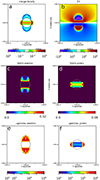 |
Fig. 1. Aligned electrosphere with surface magnetic field, B* = 109 G, rotation period, P = 10 ms, and a surface composed of electrons and protons. The inner circle represents the NS radius, R* = 12 km. The data cross section in the plane includes the rotational axis, Oz, and the magnetic axis of symmetry, except inside the inner circle where it represents data at 20 m above the surface. (a) Charge density, including the contribution of ions and electrons; (b) parallel electric field; (c) electron azimuthal velocity (normalized to the speed of light, c); (d) proton azimuthal velocity; (e) mean electron Lorentz factor; and (f) mean proton Lorentz factor. |
We can see with the charge density map Fig. 1a that the electrons form two domes, one above each pole. The protons form a small equatorial belt, or a torus. This structure with two polar domes and an equatorial belt is characteristic of all the aligned electrospheres described in the above cited literature.
The parallel electric field is plotted on Fig. 1b. The parallel electric field is characterized by two domes with a given polarity, inserted into a larger region of opposite polarity. The two regions are separated by a “polarity inversion dome” (the transition from red to blue in Fig. 1, above each polar region) where its sign reverses. This parallel field extracts the electrons at the bases of the two domes, and it extracts the protons near the equatorial plane. Then, the particles combine a motion of high velocity along the magnetic field lines with drifts guided by the corotation electric field and magnetic field line curvature. The protons are quite soon re-injected into the NS, at the hemisphere opposite to that of their emission. The electrons are accelerated above the NS surface and reach the limit of the electric polarity inversion dome, and then are accelerated back in the direction of the star. Then they again cross the electric polarity inversion dome and are decelerated. In spite of the radiative losses, most of them reach the NS. This dynamic behavior is not that of a force-free plasma, but the resulting shape of the electrosphere is very like that described in Pétri et al. (2002), which is based on the force-free hypothesis.
The total electric charge of the magnetosphere converges in about two iterations toward a value, Qt = −0.36 × 10⁻³Qc, where  . The charge, Qc, is the same (in Gaussian units) as that in Pétri et al. (2002). The domes in our simulation are smaller but comparable to the ones in Petri.
The mean azimuthal normalized velocities, vϕ/c, are plotted for the electrons in Fig. 1c and for the protons in Fig.1d. We can see, as in Pétri et al. (2002), that the proton velocity reaches its maximum at a distance on the order of a few tens of percent of the NS radius. We can also see that the electron mean velocity increases with colatitude.
The particle energies are not documented in the literature. In plots e for electrons and f for protons in Fig. 1, we can see that the Lorentz factors reach values up to 108. In the “polarity inversion dome,” the mean energy of electrons is lower by an order of magnitude. This is normal, as it’s at this point that the particles turn in the direction of the star, and therefore in the “polarity inversion domes” their parallel velocity temporarily reaches a null value and the average energy is lower.
5. Aligned electrosphere with electrostatic boundary conditions
The electric field induced by the electrosphere charge density,  , was now taken into account. A parallel magnetosphere with the same parameters as in the previous section was simulated. The stationary solution was the same, to a very high degree of accuracy. As with the vacuum boundary solution, at the second iteration, Qt = −0.36 × 10⁻³Qc. Panels a and b in both Figs. 1 and 2 show no difference. The reason is that the electric field induced by the charge volume density in the electrosphere (panels e and f of Fig. 2) reaches a maximal value of 105 statV cm−1, when the total electric field, which is mainly the vacuum solution of a rotating magnetized sphere, reaches values 1000 times larger (panels c and d of the same figure). The conclusion is that an aligned electrosphere can be set up in the low-density approximation, as was done for instance by Higgins & Henriksen (1997).
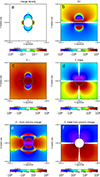 |
Fig. 2. Aligned electrosphere with the same parameters as in Fig. 1 but with internal boundary conditions that take into account the charge density of the electrosphere. Cross section of data in the plane including the axis of rotation, Oz, and the axis of magnetic symmetry, except inside the inner circle where it represents data at the surface of the NS star. (a) Charge density including ion and electron contributions; (b) parallel electric field; (c,d) radial, Er, and latitudinal, Eθ, components of the electric field; and (e,f) same components of the Eρ electrostatic electric field induced by the electrosphere’s charge density, whose value |

6. Oblique electrospheres
All the oblique electrosphere simulations presented in this section were carried out once in the  = 0 approximation and once in the
  ≠ 0 approximation. In the latter case, it systematically turns out that
  statV cm−1 when the total electric field, E> ∼ 107 statV cm−1, and apart from the value of
  , the solutions given by the two simulations do not allow us to distinguish their boundary conditions. Consequently, we no longer mention which of the two boundary conditions is used in the following presentation of oblique electrospheres.
Figure 3 shows the charge densities and parallel electric field of electrospheres with the same parameters as in Sect. 4, except for their magnetic inclination angles, which take the values i = 30° (plots a,b), i = 45° (c,d), and i = 75° (e,f). If electron-positron pair creation was effective, these parameters would correspond to a typical recycled millisecond pulsar. Figure 3 shows the electric charge densities (plots a,c,e) and the parallel electric fields (plots b,d,f).
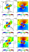 |
Fig. 3. Charge densities and parallel electric fields of oblique electrospheres with inclination angles (a,b) I = 15°, (c,d) I = 45°, and (e,f) I = 75°. The other parameters and the projections are the same as in Fig. 1. |
The structure of oblique electrospheres, with two electron domes and the proton torus, are the same as with the aligned electrosphere of Fig. 1. The parallel electric field also has the same structure. For i = 75°, the parallel electric field seems more complex, with a quadrupolar structure. Actually, the change of sign of the parallel electric, E ⋅ B/B, field is caused by an inversion of the projection of the magnetic field direction, B/B, onto the electric field and not by a inversion of the electric field polarity. Therefore, we can still speak of two main regions of an accelerating electric field separated by an intermediate torus-like region that isolates the two domes from each other. The quadrupole structure of the parallel electric field is simply an effect of the projection of E onto B.
The particle densities of electrons and of ions have been plotted separately (not shown). These plots show electrons only in the domes and protons only in the torus. Therefore, the negative charge density regions that we can see in plots a,c,d are filled only with electrons and the positive charge density regions are filled only with protons.
With i ≠ 0, the electron domes are asymmetrical, with greater extension on the side closest to the axis of rotation. Their summit lies between the magnetic axis and the rotation axis, Oz. Inside the domes, the electron density is lower than in the inversion region by a factor of ten or more. This is explained by the electron velocity, which is almost c when it enters the electrosphere and which diminishes while reversing its direction in the electric “polarity inversion dome.” The particle number conservation implies that in the low-velocity zones the particle number density is higher than in the high-velocity zones.
The size of the proton torus is an increasing function of the magnetic inclination angle, i. Nevertheless, we can notice that the color scale for densities covers a range of 104, and that when a range of only 103 is considered, the size of the domes and torus is restricted to about one NS radius.
More data characterizing the electrosphere with the inclination angle i = 75° is presented in Fig. 4. The projection angles are the same as in Fig. 3, but two scales are used. The scales are given by the circle in the center of each plot, whose diameter equals R* = 12 km. Plots a and b are the charge density and the parallel electric field, but at a larger scale. They show the large spatial extent of the low-density part of the proton belt, and the slow radial decrease of the parallel electric field. We have also checked that for distances r > 7 R*, as for a central point charge, the electric field decreases proportionally to r−2. Plot c shows the azimuthal component of the electric current. It is highly structured, and the current density causes a weak distortion of the magnetic field relative to the vacuum solution that can be noticed by examination of magnetic field lines that have their footpoints at the same magnetic latitude. In plot d the parts of the field lines closer to the observer are in white and the farther ones are in black. We can see that their shape is not symmetric relative to the magnetic axis. It is symmetric with the vacuum solution. Nevertheless, the distortion of the magnetic field is small near the NS, and the approximation used in most models, where the magnetic field is the vacuum solution, is globally correct. The parallel electric field is also different from the vacuum solution. Nevertheless, the subtraction of the parallel electrosphere electric field with the central charge electric field, Qc/r2, and the vacuum solution shows a structured pattern but with an amplitude that does not exceed a few percent of the electrosphere electric field (not shown).
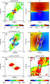 |
Fig. 4. Oblique electrospheres with inclination angle I = 75°. The other parameters and the projections are the same as in Fig. 1. (a) Electric charge density; (b) parallel electric field; (c) azimuthal current density, jϕ; (d) radial magnetic field and magnetic field lines; (e) mean electron Lorentz factor; and (f) mean proton Lorentz factor. |
The electron and proton Lorentz factors of the oblique electrospheres are not significantly different from those of the aligned electrospheres. They reach average values of a few 107 for electrons and a few 106 for protons. In terms of kinetic energies, we can notice that the protons reach larger values than the electrons. This is because the electrons lose a lot of their energy through curvature radiation, while the proton radiation loss is much weaker.
As was said in the introduction, the corotation plasma density, also called the GJ density, ρGJ, plays an important role near the NS’s surface. It corresponds to the inner boundary particle number density set in these simulations. So, by construction, the ratio, ρ/ρGJ, of the charge density over the corotation charge density is one at the NS’s surface. This ratio is plotted on the left-hand side of Fig. 5 for a pulsar with an inclination angle, i = 45° (the other parameters are the same as above). On the right-hand side, the corotation charge density is plotted. Above the NS disk, the plotted data corresponds to an altitude of 20 m above the surface. We can see that the charge density in the electrosphere is comparable to the corotation density in the proton belt, and at the outer boundaries of the electron domes. Inside the electron domes, the electrons are very fast, with the same flux as at the inner boundary; therefore, the density is weak, ρ ∼ 10−3ρGJ. It might seem strange that the electrons density does not correspond to ρGJ. Actually, it does not mean that they do not rotate with the star. When ρGJ is evaluated, it is considered that the corotating frame is a frame without acceleration. In the simulations, the accelerating parallel electric field is strong in the observer’s frame as well as in the corotating field. It is therefore not inconsistent to see a ratio, ρ/ρGJ ≠ 1, and a plasma in rotation.
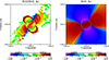 |
Fig. 5. Oblique electrospheres with inclination angle I = 45°. The other parameters and the projections are the same as in Fig. 1. (a) Electric charge density divided by the local GJ density, ρ/ρGJ; and (b) GJ density, ρGJ. |
6.1. Influence of the radiative losses and of the plasma composition
Three solutions for the perpendicular electrosphere with i = 90° are presented in Fig. 6. Here again, the plots in the left-hand-side column represent the electric charge density and those in the right-hand-side column represent the parallel electric field. In the top row (a,b), the electrosphere is simulated with an electrospheric population made of electrons and protons, as in the previously presented simulations. The middle row (c,d) represents the simulation in the same conditions, but where the particle radiation loss is not taken into account. The bottom row shows an electrosphere composed of electrons and positrons.
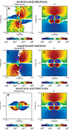 |
Fig. 6. Oblique electrospheres with inclination angle I = 90°. The other parameters and the projections are the same as in Fig. 1. Left-hand side (a,c,e): charge density. Right-hand side (b,d,f): parallel electric field. Upper row (a,b): simulation with electrons and protons and particle radiation loss. Middle row (b,c): electrons and protons and no radiation loss. Bottom row (e,f): electrons and positrons and particle radiation losses. |
Without radiation losses, the regions occupied by the electrons and by the ions have similar sizes. The electrons are not really confined in well-delimited domes. Moreover, their energies reach Lorentz factors up to a few 108. With radiation losses, mostly efficient with low-mass particles (here, electrons), the domes are smaller in size, with a clearly defined boundary.
The electrosphere made of electrons and positrons (radiation losses are taken into account) shows a quadrupole structure that was already presented in McDonald & Shearer (2009). This raises the following question: with electrons and protons, is the charge density structure a quadrupole or is it constituted of two domes and a proton torus? In Fig. 7, the projection of the electric charge density onto the planes y, z and x, z (perpendicular to the magnetic axis for i = 90°) shows a ring of protons all around the magnetic axis and two domes of electrons. With electrons and positrons, there are no particles in the y, z plane (not shown). Therefore, the dome-torus structure is present for inclination angle 0 ° ≤i ≤ 90° with electrons and protons. It becomes a quadrupole for electrons and positrons, and i = 90°.
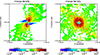 |
Fig. 7. Oblique electrospheres with inclination angle I = 90°. The other parameters are the same as in Fig. 1. Left-hand side: charge density in the plane containing the rotation axis (Oz) and the magnetic axis of symmetry (Oy for I = 90°). Right-hand side: charge density in the magnetic equatorial plane (Oxz). |
6.2. Oblique electrospheres in the pulsar graveyard
The electrosphere simulations presented in the previous sections were associated with a NS magnetic field, B* = 109 G, and a rotation period, P = 10 ms. Actually, many recycled pulsars have these characteristics. This means that in these conditions, electron-positron pair productions are sufficient to trigger an intense pulsar radiative activity. It is therefore interesting to simulate the electrospheres of NSs with lower rotational and magnetic energies because these ones, situated in the pulsar graveyard, have good chances of behaving as electrospheres and not as pulsars. Therefore, simulations of electrospheres with values of B* and P* typical of the pulsar graveyard were performed. Figure 8 shows the electric charge density, with the same projection as in Fig. 3, of an electrosphere with a surface magnetic field, B* = 1012 G, a rotation period, P* = 5 s, and an inclination angle, i = 45°. Two well-delimited electron domes and a proton torus are clearly visible.
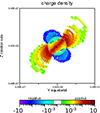 |
Fig. 8. Charge density of an electrosphere on the high-magnetic-field side of the pulsar graveyard, with B* = 1012 G, P* = 5 s, and i = 45°. |
Figure 9 shows an example of an electrosphere in the low-magnetic-field area of the P − Ṗ diagram. With B* = 108 G, a rotation period, P* = 100 ms, and i = 30°, we can still see the two domes and the proton torus. But the electron domes boundaries extend quite far from the NS. Nevertheless, the areas where the electron density is more that 0.1% of its maximal value extends only up to a distance of 4 R*.
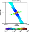 |
Fig. 9. Charge density of an electrosphere on the low-magnetic-field side of the pulsar graveyard, with B* = 108 G, P* = 100 ms, and i = 30°. |
7. Discussion and conclusion
In this paper, we have presented, for the first time, numerical simulations of oblique electrospheres of NSs with realistic parameters. Aligned electrospheres had already been modeled, using realistic parameters (such as those in Pétri et al. 2002), and two simulations of oblique electrospheres were presented with reduced parameters in one article (McDonald & Shearer 2009). The present paper is based on a significantly larger number of numerical simulations.
The most striking and immediate observation is the persistence, at any inclination angle, of the structure with two electron domes and an ion torus that has been described for aligned electrospheres since the seminal work presented in Krause-Polstorff & Michel (1985).
Another observation is that most of the previous models of electrospheres supposed that, at least at the inner boundary, right above the NS, the plasma was in force free equilibrium. The idea behind this hypothesis, as was said in McDonald & Shearer (2009), was that the low-altitude electrospheric plasma would be sufficiently dense to screen the “vacuum-like” surface electric field, and its parallel component would tend to zero. Our simulations take the finite particle inertia into account, and this does not constrain the solution to be force-free. Moreover, unlike McDonald & Shearer (2009), we did not try to reach a solution that would tend to a force-free equilibrium at the NS surface. What we can see is that the plasma density, which is on the order of the GJ density near the NS, is not high enough to screen the accelerating electric field. As a consequence, in spite of them still having two electron domes and a torus of protons, they are populated by particles that have been strongly accelerated and that propagate with very large Lorentz factors. The fact that the boundary conditions for oblique electrospheres may be not force-free may explain why only one work, with no follow-up, was published on this subject before the present study.
We have shown the existence of non-force-free solutions to the electrosphere. We have not proven their uniqueness, and it is possible that other initial set-ups could favor force-free solutions.
Because of the force-free condition that they imposed on the NS surface, Pétri et al. (2002) noticed that the total electric charge in the electrosphere, Qt, is a free parameter. They presented models of aligned electrospheres with Qt = αQc, where  and α took the values 0, 1, 3. We observe that it converges toward values that are different in every case, on the order of a few 10−2. The only exception is when the electrosphere contains electrons and positrons, and i = 90. In that case, charged particles of opposite signs play the same role, and α varies randomly around zero, with a dispersion of a few 10−3 with the
  = 0 inner boundary condition and of a few 10−6 with
  ≠ 0.
≠ 0.
The numerical methods involved in the present study are different from those used in the previous numerical studies of electrospheres and pulsars. Here are some comments on their robustness and weaknesses.
This code produces, by construction, a stationary solution. If the actual behavior of a NS environment is oscillatory, it is possible that the solutions we present are a kind of average value of the various intermediate states. However, observation of pulsars (which, in addition to the simulations in this study, contain cascades of electron-positron pairs) shows that all pulses can be different, but that an average of a few tens of pulses in most cases presents a fairly invariant pattern. From the point of view of numerical analysis, we have observed that all the parameter sets tested in the present study achieve convergence, but we do not have a general proof of convergence.
Maxwell’s equations were solved with spectral methods. These methods are very efficient as long as no sharp gradients are met in the simulations (such as spatially unresolved shock waves). With Nangles = 32, the angular resolution may seem fairly low. Simulations conducted with Nangles = 64 presented smoother solutions for a cost in memory and in a CPU multiplied by four. Nevertheless, the structure and the properties of the electrospheres computed with Nangles = 32 and with Nangles = 64 were the same; this is why we used Nangles = 32 in most simulations.
Because of the very high acceleration very near the NS surface, we used a resolution in r down to about 1 cm for the first cells. The other Nd − 1 shells were tried with various sizes, with Nd in the range of 8–11. The stability of the solution with different simulation grids confirmed the robustness of the spectral methods that we implemented.
The integration of long particle trajectories over one iteration is also a factor of efficiency. When a trajectory is long (we used Nsteps = 10 000), it can start from the NS, cross the dome of the proton belt, and go back into the NS (at a different place from where it started). There is obviously no need to restart it somewhere in the simulation domain at the following iteration. When trajectories are shorter, for instance with Nsteps = 100, for most of them the particle is still in the electrosphere when time step 100 is reached, and at the next iteration it is restarted from inside the electrosphere. It turns out that this is more costly. The solution of convergence is the same, but it is reached at a lower expense when Nsteps = 10 000, and with a lesser number of iterations.
The formalism of the charge deposition presented in Sect. 3.6 assigns each macro-particle a statistical weight proportional to the fraction, f, of the distribution it represents. Therefore, not all particles have the same statistical weight. This allows us to take into account minor populations and also allows for a wide range of particle number densities, as we can see in plots of the electric charge density.
The integration of the particle motion is quite robust. It takes finite particle inertia into account. A series of tests, where comparison with well-known theoretical solutions was possible, were conducted with success. This method of resolution is also very fast, because of the variable time steps, Δti, and because there is no need to resolve the particle gyro-period. As was said in Sect. 3.4, the domain of application of this method is larger than those of pulsars and electrospheres, and it will be presented in a further publication.
With the simplified model presented in Higgins & Henriksen (1997, 1998) it was shown that electrosphere gamma ray light curves have similarities to those of gamma ray pulsars. In the present work, the consideration of radiation effects is still poorly taken into account. We have not yet provided maps of radiated photons. This is a matter of time, and of work to be done. However, the particle energy losses by radiation are taken into account, as is described in Sect. 3.5. The method described in this section presents two drawbacks worth mentioning. The first is that the curvature, Cm, that we should use ideally is that of the trajectory, but for ease we used the curvature of the magnetic field line passing through the particle. Because of the guiding center drifts, this is not fully correct. The second drawback may have more important consequences. Sometimes (especially when B* ∼ 1012), because of the γ4 factor in the radiation loss formula, and because of the large values of γ, a numerical instability can be triggered. As was mentioned in Sect. 3.5, this instability is explosive and easy to detect. When we could detect it, we replaced the general computation of the particle Lorentz factor by a value of γa given in Eq. (3), which corresponds to an equality of the electric acceleration and the radiation loss. This does not necessarily correspond to the actual physical situation. The consideration of the radiation effects can be improved. Also, if it is clear that electrospheres contain high-energy particles, the values of the Lorentz factors reached in the simulation must be considered with care.
The simulations were all conducted on a laptop equipped with an Intel Core i7 processor. The code was parallelized in a non-scalable way. Four processes were used. The typical duration of an iteration of the simulations presented in this paper is typically a few tens of minutes, convergence is reached in about two to four iterations, and computing ten iterations requires less than four hours.
The low cost of these simulations, in terms of equipment, time, and environmental resources, opens up prospects for future developments to improve our understanding of pulsar physics. The next step will involve high-energy photon emissions from electrospheres. Then we plan to include cascades of electron-positron pairs, and hence numerical simulations of pulsars, if possible with realistic parameters. Many ways of modeling pair creation have been implemented in numerical simulations. We could for instance implement “uniform particle injection,” whereby pairs are supposed to be created in all acceleration regions. We could also try to give a better account of the microphysics of pair creations, if possible by implementing the main features demonstrated in Voisin et al. (2018). The structure of Pulsar ARoMa makes it possible to include the metrics of general relativity. The Pulsar ARoMa numerical simulation code is designed to become a versatile tool for the study of pulsar physics. Before reaching this stage, further development and validation tests are necessary, and they are underway.
Acknowledgments
I would like to thank my colleagues Silvano Bonazzola (now retired) and Guillaume Voisin for their help and support.
References
- Beskin, V. S., & Litvinov, P. E. 2022, MNRAS, 510, 2572 [NASA ADS] [CrossRef] [Google Scholar]
- Bonazzola, S., Mottez, F., & Heyvaerts, J. 2015, A&A, 573, A51 [NASA ADS] [CrossRef] [EDP Sciences] [Google Scholar]
- Cerutti, B., & Beloborodov, A. M. 2017, Space Sci. Rev., 207, 111 [NASA ADS] [CrossRef] [Google Scholar]
- Deutsch, A. J. 1955, Ann. Astrophys., 18, 1 [NASA ADS] [Google Scholar]
- Gold, T. 1968, Nature, 218, 731 [NASA ADS] [CrossRef] [Google Scholar]
- Goldreich, P., & Julian, W. H. 1969, ApJ, 157, 869 [Google Scholar]
- Grandclément, P., & Novak, J. 2009, Liv. Rev. Relat., 12, 1 [CrossRef] [Google Scholar]
- Hewish, A., Bell, S. J., Pilkington, J. D. H., Scott, P. F., & Collins, R. A. 1969, Nature, 224, 472 [NASA ADS] [CrossRef] [Google Scholar]
- Higgins, M. G., & Henriksen, R. N. 1997, MNRAS, 292, 934 [CrossRef] [Google Scholar]
- Higgins, M. G., & Henriksen, R. N. 1998, MNRAS, 295, 188 [Google Scholar]
- Krause-Polstorff, J., & Michel, F. C. 1985, A&A, 144, 72 [NASA ADS] [Google Scholar]
- McDonald, J., & Shearer, A. 2009, ApJ, 690, 13 [Google Scholar]
- Mottez, F. 2008, J. Comput. Phys., 227, 3260 [NASA ADS] [CrossRef] [Google Scholar]
- Mottez, F., Adam, J. C., & Heron, A. 1998, Comp. Phys. Commun., 113, 109 [NASA ADS] [CrossRef] [Google Scholar]
- Pacini, F. 1967, Nature, 216, 567 [NASA ADS] [CrossRef] [Google Scholar]
- Pétri, J. 2013, MNRAS, 433, 986 [CrossRef] [Google Scholar]
- Pétri, J. 2015, MNRAS, 450, 714 [CrossRef] [Google Scholar]
- Pétri, J., Heyvaerts, J., & Bonazzola, S. 2002, A&A, 384, 414 [NASA ADS] [CrossRef] [EDP Sciences] [Google Scholar]
- Philippov, A. A., & Spitkovsky, A. 2014, ApJ, 785, L33 [NASA ADS] [CrossRef] [Google Scholar]
- Riley, T. E., Watts, A. L., Ray, P. S., et al. 2021, ApJ, 918, L27 [CrossRef] [Google Scholar]
- Smith, I. A., Michel, F. C., & Thacker, P. D. 2001, MNRAS, 322, 209 [NASA ADS] [CrossRef] [Google Scholar]
- Sturrock, P. A. 1970, Nature, 227, 465 [NASA ADS] [CrossRef] [Google Scholar]
- Timokhin, A. N., & Harding, A. K. 2019, ApJ, 871, 12 [NASA ADS] [CrossRef] [Google Scholar]
- Vay, J. L. 2008, Phys. Plasmas, 15, 056701 [NASA ADS] [CrossRef] [Google Scholar]
- Voisin, G., Mottez, F., & Bonazzola, S. 2018, MNRAS, 474, 1436 [CrossRef] [Google Scholar]
All Figures
|
Fig. 1. Aligned electrosphere with surface magnetic field, B* = 109 G, rotation period, P = 10 ms, and a surface composed of electrons and protons. The inner circle represents the NS radius, R* = 12 km. The data cross section in the plane includes the rotational axis, Oz, and the magnetic axis of symmetry, except inside the inner circle where it represents data at 20 m above the surface. (a) Charge density, including the contribution of ions and electrons; (b) parallel electric field; (c) electron azimuthal velocity (normalized to the speed of light, c); (d) proton azimuthal velocity; (e) mean electron Lorentz factor; and (f) mean proton Lorentz factor. |
| In the text | |
|
Fig. 2. Aligned electrosphere with the same parameters as in Fig. 1 but with internal boundary conditions that take into account the charge density of the electrosphere. Cross section of data in the plane including the axis of rotation, Oz, and the axis of magnetic symmetry, except inside the inner circle where it represents data at the surface of the NS star. (a) Charge density including ion and electron contributions; (b) parallel electric field; (c,d) radial, Er, and latitudinal, Eθ, components of the electric field; and (e,f) same components of the Eρ electrostatic electric field induced by the electrosphere’s charge density, whose value |
| In the text | |
|
Fig. 3. Charge densities and parallel electric fields of oblique electrospheres with inclination angles (a,b) I = 15°, (c,d) I = 45°, and (e,f) I = 75°. The other parameters and the projections are the same as in Fig. 1. |
| In the text | |
|
Fig. 4. Oblique electrospheres with inclination angle I = 75°. The other parameters and the projections are the same as in Fig. 1. (a) Electric charge density; (b) parallel electric field; (c) azimuthal current density, jϕ; (d) radial magnetic field and magnetic field lines; (e) mean electron Lorentz factor; and (f) mean proton Lorentz factor. |
| In the text | |
|
Fig. 5. Oblique electrospheres with inclination angle I = 45°. The other parameters and the projections are the same as in Fig. 1. (a) Electric charge density divided by the local GJ density, ρ/ρGJ; and (b) GJ density, ρGJ. |
| In the text | |
|
Fig. 6. Oblique electrospheres with inclination angle I = 90°. The other parameters and the projections are the same as in Fig. 1. Left-hand side (a,c,e): charge density. Right-hand side (b,d,f): parallel electric field. Upper row (a,b): simulation with electrons and protons and particle radiation loss. Middle row (b,c): electrons and protons and no radiation loss. Bottom row (e,f): electrons and positrons and particle radiation losses. |
| In the text | |
|
Fig. 7. Oblique electrospheres with inclination angle I = 90°. The other parameters are the same as in Fig. 1. Left-hand side: charge density in the plane containing the rotation axis (Oz) and the magnetic axis of symmetry (Oy for I = 90°). Right-hand side: charge density in the magnetic equatorial plane (Oxz). |
| In the text | |
|
Fig. 8. Charge density of an electrosphere on the high-magnetic-field side of the pulsar graveyard, with B* = 1012 G, P* = 5 s, and i = 45°. |
| In the text | |
|
Fig. 9. Charge density of an electrosphere on the low-magnetic-field side of the pulsar graveyard, with B* = 108 G, P* = 100 ms, and i = 30°. |
| In the text | |
Current usage metrics show cumulative count of Article Views (full-text article views including HTML views, PDF and ePub downloads, according to the available data) and Abstracts Views on Vision4Press platform.
Data correspond to usage on the plateform after 2015. The current usage metrics is available 48-96 hours after online publication and is updated daily on week days.
Initial download of the metrics may take a while.