| Issue |
A&A
Volume 683, March 2024
|
|
|---|---|---|
| Article Number | A23 | |
| Number of page(s) | 17 | |
| Section | Extragalactic astronomy | |
| DOI | https://doi.org/10.1051/0004-6361/202347131 | |
| Published online | 29 February 2024 | |
Cosmic evolution of FRI and FRII sources out to z = 2.5
1
Leiden Observatory, Leiden University, PO Box 9513 2300 RA Leiden, The Netherlands
e-mail: This email address is being protected from spambots. You need JavaScript enabled to view it.
2
Institute for Astronomy, University of Edinburgh, Royal Observatory, Blackford Hill, Edinburgh EH9 3HJ, UK
3
SURF/SURFsara, Science Park 140, 1098 XG Amsterdam, The Netherlands
4
School of Physical Sciences, The Open University, Walton Hall, Milton Keynes MK7 6AA, UK
5
ASTRON, The Netherlands Institute for Radio Astronomy, Postbus 2, 7990 AA Dwingeloo, The Netherlands
6
ETH Zurich, Institute for Particle Physics and Astrophysics, Wolfgang-Pauli-Str 27, Zurich 8093, Switzerland
7
INAF-IAPS, Via Fosso del Cavaliere 100, 00133 Rome, Italy
8
Centre for Extragalactic Astronomy, Department of Physics, Durham University, Durham DH1 3LE, UK
9
Institute for Computational Cosmology, Department of Physics, University of Durham, South Road, Durham DH1 3LE, UK
Received:
8
June
2023
Accepted:
20
November
2023
Abstract
Context. Radio-loud active galactic nuclei (RLAGN) play an important role in the evolution of galaxies through the effects on their environment. The two major morphological classes are core-bright (FRI) and edge-bright (FRII) sources. With the LOw-Frequency ARray (LOFAR), we can now compare the FRI and FRII evolution down to lower flux densities and with larger samples than before.
Aims. Our aim is to examine the cosmic space density evolution for FRIs and FRIIs by analyzing their space density evolution between L150 ∼ 1024.5 W Hz−1 and L150 ∼ 1028.5 W Hz−1 and up to z = 2.5. In particular, we look at the space density enhancements and compare the FRI and FRII evolution with the total RLAGN evolution.
Methods. We constructed radio luminosity functions (RLFs) from FRI and FRII catalogues based on recent data from LOFAR at 150 MHz to study the space densities as a function of radio luminosity and redshift. These catalogues contain over 100 times the number of FRIs with associated redshifts greater than z = 0.3, compared to the most recent FRI/FRII RLF study. To derive the maximum distance according to which a source can be classified and to correct for detection limits, we conducted simulations of how sources appear across a range of redshifts.
Results. Our RLFs do not show any sharp transitions between the space density evolution of FRI and FRII sources as a function of radio luminosity and redshift. We report a space density enhancement from low to high redshift for FRI and FRII sources brighter than L150 ∼ 1027 W Hz−1. Furthermore, while we observe a tentative decrease in the space densities of FRIs with luminosities below L150 ∼ 1026 W Hz−1 and at redshifts beyond z = 0.8, this may be due to residual selection biases. The FRI/FRII space density ratio does not appear to evolve strongly as a function of radio luminosity and redshift.
Conclusions. We argue that the measured space density enhancements above L150 ∼ 1027 W Hz−1 are related to the higher gas availability in the earlier, denser universe. The constant FRI/FRII space density ratio evolution as a function of radio luminosity and redshift suggests that the jet-disruption of FRIs might be primarily caused by events occurring on scales within the host galaxy, rather than being driven by changes in the overall large-scale environment. The remaining selection biases in our results also highlight the need to resolve more sources at angular scales below 40″, thereby strengthening the motivation for further developing and automating the calibration and imaging pipeline of LOFAR data to produce images at a sub-arcsecond resolution.
Key words: galaxies: active / galaxies: evolution / galaxies: statistics / radio continuum: galaxies
© The Authors 2024
 Open Access article, published by EDP Sciences, under the terms of the Creative Commons Attribution License (https://creativecommons.org/licenses/by/4.0), which permits unrestricted use, distribution, and reproduction in any medium, provided the original work is properly cited.
This article is published in open access under the Subscribe to Open model. This email address is being protected from spambots. You need JavaScript enabled to view it. to support open access publication.
1. Introduction
It is believed that most (if not all) galaxies host a super massive black hole (SMBH; Magorrian et al. 1998; Kormendy & Ho 2013), whereby some of them are powered by an accretion disk around it (Lynden-Bell 1969; Kauffmann et al. 2003; Martini et al. 2013). We classify these objects as active galactic nuclei (AGN). They are referred to as radio-loud AGN (RLAGN) when they also produce powerful collimated jets emitting at radio frequencies, due to gas falling onto the SMBH and interacting with its magnetic field, thereby generating synchrotron emission (see review by Hardcastle & Croston 2020, and references therein). Thus, RLAGN play an important role in the evolution of the universe, as their jets heat their environment and accelerate high energy cosmic rays. They might, in fact, be responsible for a large segment of the intergalactic magnetic field (Blandford et al. 2019). In addition, RLAGN influence the evolution of their host galaxy through feedback processes, where the energy released by the AGN can prevent cooling or expel gas. This may regulate or even quench star formation and therefore affect the growth of the host galaxies (e.g., Croton et al. 2006; Best et al. 2006; McNamara & Nulsen 2007; Cattaneo et al. 2009; Fabian 2012; Morganti 2017; Hardcastle & Croston 2020). Moreover, there also seems to be a link between the radio loudness and the host morphology, where the most powerful RLAGN are hosted by massive geometrically round-shaped galaxies (Barišić et al. 2019; Zheng et al. 2020, 2022). All of the above are reasons to argue for the importance to study the cosmic evolution of RLAGN.
The morphologies of RLAGN can be classified based on the distance from the central galaxy to the brightest point of their jets (Fanaroff & Riley 1974). The two main classes are the core-bright FRI morphologies and the edge-bright FRII morphologies. Fanaroff & Riley (1974) found in their sample a ‘break luminosity’ at a radio power of L150 ∼ 1026 W Hz−1, where FRIs dominate below this luminosity value and FRIIs above. In the study by Ledlow & Owen (1996), it was demonstrated that the break luminosity increases for increasing host optical luminosity. This observation suggested a direct link between the morphology of radio jets and their environmental density. As a result, it was proposed that RLAGN initially exhibit an FRII morphology, but later transition to an FRI morphology when they are unable to traverse the local interstellar medium, which breaks the jet-collimation and decelerates the jet speed on kpc-scales from their host galaxy (Bicknell 1995; Kaiser & Best 2007). More recent studies, based on samples of radio sources less affected by selection effects compared to older studies, showed that the break luminosity does not separate FRI and FRII morphologies as strictly as was initially observed (Best 2009; Gendre et al. 2010, 2013; Wing & Blanton 2011; Capetti et al. 2017b; Mingo et al. 2019, 2022). The FRI/FRII morphological divide is therefore less closely connected to radio luminosities than previously suspected. Nonetheless, the existence of FRII below the original break luminosity remains consistent with the jet-disruption model if this population is a mix of restarting FRIIs, (old) fading FRIIs, or FRIIs hosted by less massive host galaxies in less dense environments compared to FRIIs above the break luminosity (Croston et al. 2019; Mingo et al. 2019). Examining the cosmic evolution of FRI and FRII morphologies is therefore linked to studies of the evolution of the large-scale environments of radio galaxies (e.g., Croston et al. 2019).
The changing interpretation of the break luminosity demonstrates how selection biases play an important role in the ability to detect FRI and FRII sources and then affect our understanding of radio galaxy evolution as a result. Because FRIIs have hotspots at the edge of the lobes and are more powerful, they will be easier to detect than FRIs. This selection effect becomes stronger when we look at more distant RLAGN, where their jets become fainter and are closer to the flux density limit from the used instrument of the survey. It has been debated how much of the observed evolution of the FRI and FRII sources is due to selection effects and how much is due to true evolution of the radio galaxy population (Singal & Rajpurohit 2014; Magliocchetti 2022). The difficulty in detecting FRIs at high redshifts, with very limited sample sizes, has led to the prediction that powerful FRIs should be significantly more abundant at z > 1 compared to what we find locally (Snellen & Best 2001; Jamrozy 2004; Rigby et al. 2008). A broader study of the FR dichotomy, with the combined NVSS-FIRST (CoNFIG) catalogue (Gendre & Wall 2008), has strengthened this prediction by finding positive space density enhancements from low to high redshift up to a factor of 10 over the local population for both FRIs and FRIIs up to z = 2.5 (Gendre et al. 2010, 2013). To understand the role of extended RLAGN across cosmic time, it is vital to fully characterise the cosmic evolution of the FRI and FRII sources using much larger samples and down to fainter radio luminosities than previous studies.
In this paper, we investigate the FRI/FRII space density evolution as a function of redshift and radio luminosity by constructing radio luminosity functions (RLFs) up to z = 2.5 with the catalogues from Mingo et al. (2019, 2022). These catalogues are based on the 150-MHz LOw-Frequency ARray (LOFAR; van Haarlem et al. 2013) surveys that have a high surface brightness sensitivity and are therefore great at detecting FRIs with low flux densities. By correcting more precisely for selection effects through redshift simulations, we derive better estimates of the maximum volume that a source can still be observed and classified over, before falling below the detection and selection limits of the sample. These simulations, in combination with the theoretical angular size distribution, help us to better correct for the incompleteness of over sample, such that we can recover an improved estimate of the ‘real’ FRI/FRII RLFs. This comprehensive approach, along with 100 times more FRI redshifts above z = 0.3 compared to previous works from Gendre et al. (2010), is also helpful in improving the FRI and FRII RLF comparisons above this redshift and to re-examine the findings from Gendre et al. (2010) regarding the space density enhancements of FRIs and FRIIs up to z = 2.5.
In Sect. 2 of this paper, we briefly discuss the selected data and catalogues. This is followed by an explanation of our redshift simulation in Sect. 3, which is then applied in Sect. 4 to construct RLFs. We present our results in Sect. 5. We further discuss our results in Sect. 6 and look at future prospects to improve this work in the future. Finally, we give our conclusions in Sect. 7. Throughout this work, we use a ΛCDM cosmology model with H0 = 70 km s−1 Mpc−1, Ωm = 0.3, and ΩΛ = 0.7.
2. Data
We utilized FRI/FRII sources classified by Mingo et al. (2019, with their catalogue hereafter referred to as M19,) combined with a similarly compiled catalogue based on deeper observations from Mingo et al. (2022, with their catalogue hereafter referred to as M22). Both catalogues were constructed with data from the LOFAR Two-metre Sky Survey (LoTSS, Shimwell et al. 2017, 2019) at 144 MHz with a resolution of 6″ and a sensitivity ranging from ∼20 to ∼70 μJy beam−1. The sensitive low-frequency observations used to construct these catalogues excel in identifying complex extended sources, which benefits the detection of extended diffuse jets from FRIs. In the following subsections, we discuss their content and our source selection.
2.1. Catalogues
Sources from LoTSS DR1 are included in M19, based on radio maps from the HETDEX Spring Field, covering 424 deg2 with a median sensitivity of 71 μJy beam−1 (Shimwell et al. 2017, 2019; Williams et al. 2019), while M22 contains sources from the LoTSS-Deep Fields DR1, which are about three to four times deeper than LoTSS DR1 and covers 25 deg2 (Tasse et al. 2021; Sabater et al. 2021; Kondapally et al. 2021; Duncan et al. 2021; Best et al. 2023). The deep fields were selected with deep wide-area multi-wavelength imaging from ultraviolet to far-infrared (see Kondapally et al. 2021 for details), consisting of the following three fields: European Large Area Infrared Space Observatory Survey-North 1 (ELAIS-N1; Oliver et al. 2000), Lockman Hole (Lockman et al. 1986), and Boötes (Jannuzi & Dey 1999). The corresponding LoTSS-Deep Fields DR1 radio maps respectively exhibit a median sensitivity of about 20, 22, and 32 μJy beam−1 for ELAIS-N1, Lockman Hole, and Boötes (Tasse et al. 2021; Sabater et al. 2021).
For every source, the M19 and M22 catalogues contain their total 150-MHz flux density, size, and host galaxy redshift and position on the sky. The sizes and radio flux densities from sources in M19 and M22 were carefully measured by adopting a flood-filling procedure and by comparing their sizes and flux densities with what was found with the PyBDSF Gaussian fitting tool (see for more details Sect. 2.5 in Mingo et al. 2019)1. These comparisons were followed up by visual inspection. The sources from the catalogue from LoTSS DR1 to construct M19 are for 73% identified with an optical host (Williams et al. 2019) and have 51% spectroscopic or photometric redshifts (Duncan et al. 2019). Sources in the deep fields were over ∼97% identified with radio host-galaxies associated with carefully determined photometric redshifts (or spectroscopic where available) using a hybrid approach of template fitting and machine learning methods (Duncan et al. 2019, 2021). Mingo et al. (2022) included in M22 only sources from the deep fields up to z = 2.5, as the spectral energy distribution (SED) fitting of all the detected radio sources in the deep fields was considered reliable for sources up to this redshift (Best et al. 2023). The FRI and FRII classifications of these sources were done using the LoMorph classification code and by additional visual inspection (Mingo et al. 2019)2. They reported a classification accuracy of 89% for FRIs and 96% for FRIIs. Mingo et al. (2019) exclude sources with projected angular sizes smaller than 27″ or below 40″, with a 20″ or smaller distance between their two peak emissions. This angular size cut is based on classification difficulties and the resolution limits from LoTSS DR1 and the LoTSS-Deep Fields DR1. Also, other sources that did not clearly fit in FRI or FRII sources were filtered out (see Sect. 2.4 from Mingo et al. 2019). Those contain double-double sources (restarting FRII; Schoenmakers et al. 2000) and hybrid sources (Gopal-Krishna & Wiita 2000).
2.2. Source selection
The sources from M19 with reliable redshifts above z = 0.8 are primarily quasars. This is mainly due to the scarcity of spectroscopic data for radio galaxies and the line-of-sight bias (Duncan et al. 2019; Hardcastle et al. 2019). As a result, we have excluded sources with redshifts beyond z = 0.8 from M19. We do not need to make additional redshift cuts for M22, as the radio galaxies from M22 are drawn from the significantly deeper LoTSS-Deep Fields DR1, in contrast to LoTSS DR1, which offers precise redshifts up to z = 2.5 (Kondapally et al. 2021; Duncan et al. 2021; Best et al. 2023). Consequently, all the sources utilized in this paper with redshifts between z = 0.8 and z = 2.5 originate exclusively from M22 and make up only ∼9% of our full sample. Although the sources collected from the LoTSS-Deep Fields DR1 have a higher redshift completeness than the sources collected from LoTSS DR1, we find the ratio of the number of FRI/FRIIs for the overlapping redshifts below z < 0.8 for M19 and M22 to be similar. Also, the redshift distributions below z < 0.8 are similar, that is, we find their redshifts to have the same mean and standard deviation. This demonstrates that combining M19 and M22 does not introduce additional selection effects as a function of redshift.
In Fig. 1, we plot the angular size versus the radio flux density and redshift for all our FRIs and FRIIs. From this figure, we see that due to the selection criteria by Mingo et al. (2019), there are very few sources between 27″ and 40″ in the sources from M19 and M22. Most of those sources are below z = 0.8. We also find a clear gap of sources above 400″, where only 0.3% of our sources are situated. This is the area where classification of bright giant radio galaxies (GRGs) becomes difficult because different selection biases for FRIs and FRIIs do play a role in relation to the surface brightness sensitivity of the used observation. First of all, the most distant parts of the FRI jets are close to or below the surface brightness limit, which (in some cases) would make only their unresolved core appear or make the measurements of their sizes smaller than they actually are. This issue becomes more prominent at the higher end of our redshift distribution where surface brightness limits play a more dominant role due to the fact that sources are on average fainter as a function of redshift. This effect can also be observed in the right panel of Fig. 1, where FRIs are closer positioned to the 40″ boundary compared to FRIIs at higher redshifts. Secondly, large FRII jets close to the surface brightness limit might appear to only have two bright disconnected hotspots. This poses challenges in associating them with each other, particularly when their separation is substantial. So, it is not unexpected that a significant proportion of large sources are missing in our catalogues (e.g., Oei et al. 2023). To account for the 40″ and 400″ angular size limits, we excluded sources that fall below and above these threshold values and subsequently implemented completeness corrections as a function of angular size and flux density to regain the contribution of sources beyond these boundaries to our RLFs, as we discuss in more detail in Sect. 4.2.2.
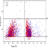 |
Fig. 1. Angular size as a function of flux density (left panel) and redshift (right panel) for the 1560 sources considered in this paper. We separated our sources into 1146 FRI and 414 FRII morphologies with separated colors and draw dashed lines for 40″ and 400″. These lines determine the angular size cuts that we applied in this paper before doing completeness corrections (see Sect. 4.2). |
We further limited our analyses to sources with a radio luminosity above L150 ∼ 1024.5 W Hz−1, as the number of sources below this radio luminosity is small. This also ensures that our completeness corrections are not strongly affected by star-forming galaxies (e.g., Sabater et al. 2019; Cochrane et al. 2023) or compact sources (e.g., Sadler 2016; Baldi et al. 2018; O’Dea & Saikia 2021). Moreover, due to the LoTSS flux density limits, beyond z = 0.8, we did not find any sources below L150 ∼ 1024.5 W Hz−1. Thus, this decision improves the reliability of completeness corrections and, therefore, our resulting RLFs without compromising the goal of this paper, which is to investigate the evolution of radio galaxies across redshifts up to z = 2.5. Figure 2 shows the final selection of the 1560 sources with their 150 MHz radio luminosities as a function of redshift. From those, 1146 are classified as FRI sources and 414 as FRII sources.
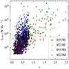 |
Fig. 2. Luminosity–redshift diagram for M19 and M22 split in FRIs and FRIIs. |
3. Redshift simulations
Detection limits from radio telescopes restrict our view of the universe. In order to incorporate these effects into the derivation of RLFs for FRIs and FRIIs, we have developed an algorithm that simulates how sources would appear after relocating them to higher redshifts, so that we can derive up to which maximum distance a source remains reliably classifiable. These redshift simulations will also help us to determine the incompleteness of our sample as a function of flux density and redshift.
3.1. Surface brightness and redshift relation
We can relate the total flux density (Sν) of a source to its luminosity (Lν) and its luminosity distance (dL) as:
 (1)
(1)
where (1 + z)1 − α accounts for the K-correction with spectral index α and where the radio flux density is Sν ∝ ν−α. The angular size θz of a source is related to its physical size s and the angular distance (dA) as:
 (2)
(2)
where we used the relation  . Combining the above, we derive the surface brightness evolution over redshift as:
 (3)
(3)
As the luminosity and physical size are physical intrinsic properties of a radio galaxy, this demonstrates that the surface brightness decreases over redshift by a factor (1 + z)3 + α.
3.2. Redshifting algorithm
If we could relocate a source to a higher redshift, we would see the angular size and flux density from the source in the image change. The source would diminish in size according to the adopted cosmology until approximately z ∼ 1.6, after which it would begin to increase once again. These angular size changes affect the ability to detect and classify FRIs and FRIIs at the same radio powers differently, due to their different morphologies. On the one hand, the FRI will be classifiable until the diffuse jets are not bright enough to be detected or the source cannot be resolved anymore due to its small angular size. On the other hand, the FRII remains classifiable as long as the hotspots appear as point sources, the components can be associated with the host, and we have the adequate resolution to separate them, while they are still bright enough above the noise. Additionally, there are situations where FR classifications can change after redshift increments from FRI to FRII and vice versa, due to the detection limits and the changing number of pixels covering the source. To simulate and better understand these effects, we developed the redshifting algorithm to increment their redshift by Δz3.
The redshifting algorithm takes as input an image of a source at its observed redshift. After every redshift increment, the algorithm changes the pixel sizes by multiplying the pixel scale via  , which is equivalent to dividing the pixel scale by the ratio between dA at z and dA at z + Δz. This information is used to resample the image pixels with the DeForest (2004) resampling algorithm4. In this way, the source appears smaller or larger after redshift increments, depending on the redshift. Following from Eq. (3), the algorithm reduces every pixel value by a factor
  . Because the image noise is independent from the source’s redshift, we kept it constant during our procedure of relocating a source to a higher redshift. This means for our algorithm that we only reduce pixel values that exceed our 3σ noise threshold.
We adopted a constant spectral index of α = 0.7 for the K-correction. This spectral index value is the typical average spectral index for RLAGN and often used to construct radio luminosity functions if the spectral indices of sources are unknown (e.g., Condon et al. 2002; Mauch & Sadler 2007; Padovani 2016; Prescott et al. 2016; Hardcastle et al. 2016; Calistro Rivera et al. 2017; Kondapally et al. 2022). A typical spectral index variation between α = 0.6 or α = 0.8 (e.g., Hardcastle et al. 2016; Calistro Rivera et al. 2017; Murphy et al. 2017) would (compared to α = 0.7) only adjust the pixel brightness changes from our redshifting algorithm up to ∼5% for redshift increments of Δz = 0.7. This is the mean Δz from their original z where we find that sources are still classifiable after applying the redshifting algorithm (see the following sections) for the sources considered in this paper. Hence, it is not expected that the choice for α = 0.7 will strongly bias our results.
We also made sure that the total power remains constant as a function of redshift increments. This implies that we do not correct for inverse Compton (IC) scattering losses from the cosmic microwave background (CMB), which is expected to add additional selection biases (Krolik & Chen 1991; Morabito & Harwood 2018; Sweijen et al. 2022a). We further discuss this aspect in Sect. 6.1 regarding the implications of this choice on the interpretation of our RLFs when we do not consider this effect.
3.3. Source components
The association of radio source components is a difficult task and massive visual inspection through citizen science projects or neural network architectures are often used to do this for large amounts of data (Banfield et al. 2015; Williams et al. 2019; Mostert et al. 2022)5. For all our sources, we already have initial information about the source components (based on PyBDSF and visual inspection, see Mingo et al. 2019). So, an additional step for associating source components is not necessary, as our focus is solely set on determining the components that remain above the noise threshold at each redshift increment. All unassociated components in the image are masked out in every source cutout image. This is necessary when multiple radio sources are close to each other, or when there are remaining islands of emission contaminating the image for classification. After relocating a source to a new redshift with redshifting, we draw polygons around the remaining components with emission above a particular noise level.
The sources in Figs. 3 and 4 demonstrate the effect of the redshifting increments on the observed morphology for different FRIs and FRIIs. We see, in particular, how their brightness is reduced and how their appearance changes. The first two rows of Fig. 3 display FRI sources, where their jets partly disappear below the σ-threshold when they are relocated at higher redshifts. In the last row, we have a special case where an FRI source appears as an FRII after large redshift increments. The sources in Fig. 4 are typical cases of FRIIs with clear hotspots. These sources are showing how the FRII hotspots are the main components that remain visible after relocating them at higher redshifts. We can see from the first and the last row how the elongated FRII component separates into two components at higher redshifts.
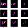 |
Fig. 3. Examples of FRI sources after redshift increments by applying the redshifting algorithm. All unassociated emission is masked out (in this case below 4σ). Each columns displays the source from the same row at different redshifts. The last row is a wide-angle tail FRI source (Owen & Rudnick 1976), where after redshift increments, the source appears to resemble an FRII source. The optical host location is in every image given by the green cross. (a) FRI at z = 0.48, (b) FRI at z = 0.93, (c) FRI at z = 1.38, (d) FRI at z = 0.19, (e) FRI at z = 0.39, (f) FRI at z = 0.59, (g) FRI at z = 0.29, (h) FRI at z = 0.69, (i) FRI at z = 1.19. |
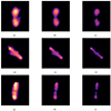 |
Fig. 4. Examples of FRII sources after redshift increments by applying the redshifting algorithm. All unassociated emission is masked out (in this case below 4σ). Each column displays the source from the same row at different redshifts. The optical host location is in every image given by the green cross. (a) FRII at z = 0.33, (b) FRII at z = 0.83, (c) FRII at z = 1.33, (d) FRII at z = 0.9, (e) FRII at z = 1.5, (f) FRII at z = 2.1, (g) FRII at z = 0.34, (h) FRII at z = 1.34, (i) FRII at z = 1.84. |
3.4. FR classification
Because we use only sources from M19 and M22, we based our FRI/FRII classification code on the LoMorph code, which were used to classify our sources. This classification algorithm is based on measuring the distance from the optical host to the brightest region and the edge of the source by using flood-filling and verifying if a source is resolved or unresolved by applying PyBDSF. For a more detailed discussion, we refer to Sect. 2 from Mingo et al. (2019).
The classification of the source on the third row in Fig. 3 changes both visually and in our algorithm from an FRI to an FRII morphology after being incremented to a higher redshift. This classification inconsistency occurs for about ∼2% of all our sources when relocating them to higher redshifts. FRIIs could also become classified as FRIs due to the resampling of pixels, when the hotspots of an FRII would merge into a bright FRI type core. We did not find such cases in our simulations, indicating that before this occurs, the source would no longer be classifiable. This could also be because double-double and hybrid sources have already been all filtered out from our sources (see Sect. 2.2 and Mingo et al. 2019, 2022). These classification inconsistencies are rare and thus demonstrates that our morphological classification is generally effective.
4. Constructing radio luminosity functions
RLFs are an important tool in studying the evolution of radio sources as a function of power and redshift. To construct the RLFs in this paper, we used the standard method from Schmidt (1968). This means that we calculated the density evolution as a function of redshift z and radio luminosity L via:
 (4)
(4)
where Vmax, n is the maximum volume that source n can be classified and where Δlog L is the log value of the radio luminosity bin. In the next subsections, we further discuss the Vmax and the completeness corrections we applied to constructing the RLFs.
4.1. Vmax method
To determine Vmax, we first need to find an accurate value for the maximum redshift at which a source can still be classified (zmax). This value can be found by applying the redshifting algorithm discussed in Sect. 3.2.
4.1.1. Determining zmax
We find zmax by spatially relocating each source across the radio image 200 times and re-evaluating up to which maximum redshift the source is still classifiable at each spatial location with the redshifting algorithm ( ). In this way, we get a reliable measure for zmax by taking the mean of all the obtained
  values and can find the error on this value by taking the standard deviation of the
  values (σzmax). The value for σzmax embeds information about the effects of the varying noise in the radio maps.
With the obtained zmax values, we can compare how FRIs and FRIIs are differently affected by the redshifting algorithm. For this, we can for example take a local sample up to z = 0.5 and move those up to z = 2.5. In Fig. 5 we show from this example the fraction of the remaining sources that are still detectable and classifiable in steps of z = 0.1. Only 50% of the FRI sources we start with remain classifiable up to z ∼ 0.6, while for FRII sources we still classify 50% of the sources up to z ∼ 1. This is partly explained by the different effects detection limits have on the observed morphologies of FRI and FRII sources (see Sect. 3.2). In addition, FRII sources are on average also brighter as they are locally more abundant above the break luminosity (Fanaroff & Riley 1974; Mingo et al. 2019). We demonstrate this in Fig. 6 where we show how 150 randomly picked sources move in P − z space from their original observed z-position to their zmax position. On the higher luminosity end, we observe, as expected, how FRII sources reach higher zmax values.
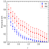 |
Fig. 5. Fraction of local (z < 0.5) FRI and FRII sources that are still classifiable after applying redshift increments with the redshifting algorithm as a function of redshift. The error bars include the errors on zmax and Poisson errors. |
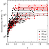 |
Fig. 6. Luminosity versus redshift increments with the redshifting algorithm for 150 random sources at different luminosities from all sources from M19 and M22 above L150 ∼ 1022 W Hz−1. The starting positions are at the original measured redshifts given by the squared boxes, while the ending positions are the final maximum redshifts a source can be classified (up to z = 2.5). |
4.1.2. Final integral for Vmax
The zmax determines the maximum redshift a source can be observed in for each redshift bin, zbin, over which we evaluate the following integral
 (5)
(5)
where C(Sν) is the completeness correction as a function of flux density at a particular redshift (see Sect. 4.2), then V(z)dz is the infinitesimal comoving volume slice between z and z + dz, Θ(z) is the fractional sky coverage, while χ(z) is the binary function:
The uncertainties on zmax propagate in Vmax by calculating  corresponding to every
  with Eq. (5) and taking the standard deviation of all the obtained values. The final uncertainties of the space densities also include Poisson errors following from Gehrels (1986) and the LoMorph classification accuracies from Mingo et al. (2019; 89% for the FRIs and 96% for the FRIIs).
As Fig. 5 demonstrates how the FRIs are more strongly affected by selection effects, it also shows how with our Vmax method the FRI space densities will be more strongly corrected as a function of z, compared to the space densities from FRII sources.
4.2. Completeness corrections
The Vmax method enables measuring the space densities for sources within our sample as a function of redshift. We also need to apply a correction that takes into account the sources that are undetected due to the flux density and resolution limits from our observations. This is the (in)completeness factor as defined in Eq. (5) by C(Sν). For this work, this means that we need to estimate how many FRI and FRII sources we are missing as a function of flux density (S150), such that we can better estimate the real space density values. Firstly, we calculate the completeness corrections by generating mock sources based on the sources from our source sample. Secondly, we determine the completeness correction for the sources with sizes below 40″ and above 400″. Combining both corrections gives our final completeness correction.
4.2.1. Correction for 40″ < θ < 400″
We find the completeness corrections from our sources as a function of flux density by first generating mock FRI and FRII sources. Those mock sources are created by multiplying the flux density from a source in our catalogue with a random factor loguniformly drawn between 0 and 1 and scaling the pixel brightness in our image with the same factor. We then replace the mock source to the same noise environments as the noise effects are already embedded in the σzmax values. When we do this 200 times per source, we have about ∼350 k mock sources. Using the classification part from Sect. 3.4, we decide for each case if it is still recoverable as an FRI or FRII source. As the M19 and M22 samples have different sensitivities, we do this for both catalogues separately. With these simulations, we find the flux density incompleteness for sources corresponding to the angular size distribution from the objects in our combined M19 and M22 catalogues.
4.2.2. Correction for θ < 40″ and θ > 400″
As explained in Sect. 2.2, we miss sources smaller than 40″ and larger than 400″. To quantify the angular size incompleteness in our completeness weights, we use the empirical integral angular size distribution from Windhorst et al. (1990) with the updated parameters fitted to LoTSS-Deep Fields DR1 by Mandal et al. (2021). This is a radio source angular size distribution which has been used in multiple studies and has proven to be a reliable measure (Prandoni et al. 2001, 2018; Huynh et al. 2005; Hales et al. 2014; Mahony et al. 2016; Williams et al. 2016; Retana-Montenegro et al. 2018; Mandal et al. 2021; Kondapally et al. 2022). The angular size distribution follows as:
 (6)
(6)
where θ is in arcseconds and where  is the median angular size which Windhorst et al. (1990) derived to be related to the flux density S1400 in mJy via
 (7)
(7)
where  and
and
where we doubled the value of k compared to Mandal et al. (2021), as Kondapally et al. (2022) showed for LoTSS-Deep Fields data the angular size distribution to fit well for AGN with twice the median angular size. By converting Eq. (7) from ν = 1.4 GHz to ν = 150 MHz, using a spectral index of α = 0.7, and combining this with Eq. (6), we find the angular size distribution as a function of the flux density S150.
The radio luminosity cut below L150 = 1024.5 W Hz−1 (see Sect. 2.2) ensures that the angular size completeness corrections are dominated by extended radio sources. Nonetheless, we cannot distinguish with the angular size distribution from Windhorst et al. (1990) the distributions of FRIs and FRIIs. Fortunately, considering the comparison of FRI and FRII physical size distributions by Best (2009), it is reasonable to infer that both morphologies have comparable size distributions. Best (2009) used data from FIRST and NVSS to show that above 40 kpc, the size distributions of FRI and FRII radio galaxies are similar, whereas the smallest source in our sample is 83 kpc and 95% of our sources are larger than 230 kpc. However, the measured angular sizes from FRIs are likely to be more underestimated at higher redshifts, as sources become dimmer as a function of redshift, which affects the detectibility of the full extend of diffuse FRI jets. As a result, the angular size completeness corrections for FRIs might become less accurate for higher redshifts, compared to FRIIs whose sizes are defined by their brightest components. However, to simplify the construction of the RLFs, we rely only on the measured angular sizes to determine the angular size completeness corrections and, therefore, we do not derive a redshift dependency. The effect of this issue on our RLFs is discussed in Sect. 6.2.
4.2.3. Final completeness correction
We present our final full completeness corrections (including all corrections discussed above) as a function of flux density in Fig. 7. We identified a 50% completeness around ∼100 mJy. This is also the flux density after which the completeness corrections start to be dominated by the angular size completeness corrections. This becomes evident in the convergence of the completeness for FRI and FRII sources at the upper end of the flux densities, stemming from the assumption of comparable size distribution for both FRIs and FRIIs. The flattening at the end of the completeness curve is showing the effects of the 400″ upper angular size threshold that becomes more dominant at higher flux densities. After 10 Jy, the completeness corrections start to fall off, which matches with the assumption that a notable fraction bright GRGs are missing due to selection effects (see Sect. 2.2). Below ∼100 mJy we notice how the better surface brightness sensitivity in LoTSS-Deep Fields DR1, compared to LoTSS DR1, improves the completeness from M22. For M19, we also notice how FRII sources at lower flux densities are more complete compared to FRI sources. This is because the FRI jets tend to be diffuser and more likely to disappear below the detection limit, while an FRII with the same flux density will typically remain classifiable as long as their prominent hotspots remain visible. Because the completeness corrections become extremely large at the lower radio flux density end, we set, similarly to the work by Kondapally et al. (2022), a lower boundary for the completeness corrections by a factor of 10. This threshold ensures that the corrections do not become unreliable large for sources at the lower flux density end of our catalogues.
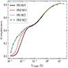 |
Fig. 7. Completeness corrections for FRI and FRII sources from M19 and M22. |
In Appendix A, we discuss a few tests to validate the RLF construction method and test the reliability of our Vmax derivations and completeness corrections with a local sample. These tests show that both the Vmax and the completeness corrections are applied well and we recover a good estimate of the space densities of FRIs and FRIIs.
5. Results
Gathering all the ingredients from Sects. 3 and 4, we constructed RLFs to study the FRI and FRII space density evolution between 1024.5 ≲ L150 ≲ 1028.5 W Hz−1 out to z = 2.5. In this section, we present our main results, where we look separately at the local RLF and the RLF up to z = 2.5.
5.1. Local radio luminosity function
The local RLF constructed with the M19 and M22 sources below z = 0.3 is shown in Fig. 8 and tabulated in Table 2. In this same figure, we also plot the FRI and FRII RLFs from Gendre et al. (2013) and the total ‘radio-excess AGN’ RLF from Kondapally et al. (2022, hereafter referred to as the total RLAGN RLF). We observe how all our local FRI and FRII space densities are near or below the total RLAGN space densities, which is constructed on the basis of all RLAGN form the LoTSS-Deep Fields DR1 (Kondapally et al. 2021; Duncan et al. 2021; Tasse et al. 2021; Sabater et al. 2021). This is an important requirement, as the FRIs and FRIIs are a subset of the total RLAGN population. The FRI and FRII RLFs from Gendre et al. (2013) also agree well with our RLFs, which is another indication that our completeness corrections are working well (see also the tests in Appendix A). The FRIs dominate below the break luminosity (L150 ∼ 1026 W Hz−1), while FRIIs dominate above. This is consistent with prior research (Fanaroff & Riley 1974; Parma et al. 1996; Ledlow & Owen 1996; Gendre et al. 2010). Similarly to Gendre et al. (2010, 2013), we find a smooth transition from the FRI to FRII dominance around the original break luminosity, where the FRI RLF drops off more strongly towards the higher radio luminosities compared to the FRII RLF. This smooth transition is also consistent with the FRI and FRII populations observed by FIRST (Capetti et al. 2017a,b).
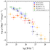 |
Fig. 8. Local RLF for FRIs and FRIIs from this paper are plotted in blue and red, respectively. For comparison and to validate that our FRI and FRII space densities do not extend above the total RLAGN population, we added the total local RLAGN RLF from Kondapally et al. (2022) beyond L150 ∼ 1024 W Hz−1 (in green). This total RLAGN RLF is constructed based on sources from the LoTSS-Deep Fields DR1. To demonstrate that our results agree with previous work, we also added the FRI and FRII RLF from Gendre et al. (2013) in black and orange, respectively. These points are based on the CoNFIG catalogue (Gendre & Wall 2008; Gendre et al. 2010), where we converted the luminosity bins to 150 MHz by using a spectral index of α = 0.7. The 1σ bars from our RLFs are including zmax errors, Poisson errors, completeness corrections errors, and classification errors. All our data points are given in Table 2. |
We can quantify the steepness of the space density drop-off after the break luminosity by fitting a broken power law. To constrain better the power-law, we include the FRI and FRII data points from Gendre et al. for the radio luminosities where our RLFs do not cover (see Fig. 8). This broken power-law is given by:
 (8)
(8)
where α and β are respectively the low and high luminosity exponents, ρ0 is the characteristic space density, and  is the break luminosity. In Table 1, we give our best fit parameters for both the local FRI and FRII fit. We see from these values how the local FRI space densities are declining more strongly towards higher radio luminosities compared to the FRIIs. We also find different values for
  , which is usually taken to be equal to the break luminosity and determined by visual inspection, as done by Gendre et al. (2010). Despite this different choice, the values for
  are still consistent with the break luminosity around ∼L150 ∼ 1026 W Hz−1 we find in the literature (e.g., Fanaroff & Riley 1974; Jackson & Wall 1999; Willott et al. 2001; Kaiser & Best 2007; Mingo et al. 2019).
5.2. Radio luminosity function up to z = 2.5
In Fig. 9, we see both the FRI and FRII space density as well as the total RLAGN from Kondapally et al. (2022). Similarly to the local RLF in Fig. 8, we find in Fig. 9 that the space densities from the FRI and FRII samples are below the total RLAGN RLF. We see for the redshift bins below z = 0.8 a break luminosity, where FRIs dominate below and FRIIs above L150 ∼ 1026 W Hz−1. Beyond z = 0.8 the break luminosity becomes less well-defined. In addition to Fig. 9, in Fig. 10 (right panel) we compare the space density evolutions per morphology class for three redshift bins, where the local RLF is fitted with a broken power-law as explained in the previous subsection. By subtracting the space densities from the FRIs and FRIIs in log space and propagating their error bars, we get the FRI/FRII ratio evolution in the left panel of this same figure. We combined all sources between z = 0.8 and z = 2.5 in one redshift bin because we have only 112 out of the total 1560 sources in this redshift range.
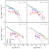 |
Fig. 9. RLF for FRI (blue) and FRII (red) sources split in different redshift bins. For comparison and to show that our FRI and FRII space densities do not extend above the total RLAGN population, we added the total RLAGN RLF from Kondapally et al. (2022) beyond L150 ∼ 1024 W Hz−1 in green. We also added the local RLFs for both FRIs and FRIIs with dot-dashed lines. We removed radio luminosity bins which only contain a single source. The 1σ bars from our RLFs are including zmax errors, Poisson errors, completeness corrections errors, and classification errors, as explained in Sects. 4.1.2 and 4.2. Data points are given in Table 2. |
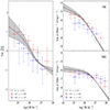 |
Fig. 10. RLF ratio evolution. Left: ratio evolution over different redshift bins. Right: separated FRI (above) and FRII (below) space density evolution plots corresponding to the ratio evolution plot in the left panel. In both figures, we added the Gendre et al. (2013) data points for the higher end of the luminosity range, such that we can further constrain the local RLF, which was fitted with a broken power law from Eq. (8) and corresponding values from Table 1, where we used a 1σ confidence interval. We removed radio luminosity bins which only contain a single source. The 1σ bars from our RLFs are including zmax errors, Poisson errors, completeness corrections errors, and classification errors, as explained in Sects. 4.1.2 and 4.2. |
In Fig. 10, we see the FRII space densities decrease at a lower rate as a function of radio luminosity when we make a comparison the highest with the lowest redshift bin. Above L150 ∼ 1027 W Hz−1, this results in a clear space density enhancement across redshift by ∼ 0.6 − 1 dex between the local and z > 0.8 RLFs. Also Gendre et al. (2010) found for FRIIs a similar space density enhancement above L150 ∼ 1027 W Hz−1, where we converted their luminosities from 1.4 GHz to 150 MHz with a spectral index of α = 0.7. They also report space density enhancements for FRIs at those radio luminosities, which also agrees with the mild enhancements that we detect.
In the right panel of Fig. 10, we detect a space density decline for FRIs from the local (z < 0.3) to the highest redshift bin (0.8 < z < 2.5) below L150 ∼ 1026 W Hz−1. For FRIIs, we do not find a significant space density decline below this radio luminosity. The space density decline for FRIs is not reported by Gendre et al. (2010). Nonetheless, both our results are still in agreement with each other within the error margin, as Gendre et al. (2010) only relied on 7 FRIs with associated redshifts above z = 0.3, making their uncertainties large. Despite the FRI space density decline beyond z = 0.8, we find the FRI/FRII space density ratios as a function of radio luminosity to remain fairly constant within error bars in the left panel of Fig. 10.
The different space density evolutions as a function of redshift are also shown in Fig. 11, where we inverted the RLFs to space density evolutions as a function of redshift for radio luminosity bins. Between 1027 ≲ L150 ≲ 1028 W Hz−1 we find a (mild) space density enhancement for both FRIs and FRIIs, which finds its maximum around z = 1.6. The space densities for FRIs and FRIIs do not show any notable redshift evolution between 1026 ≲ L150 ≲ 1027 W Hz−1. For FRIs, we find a mild space density decline above z ∼ 0.6 and between 1025 ≲ L150 ≲ 1026 W Hz−1, while FRIIs do show for these radio luminosities hints of a mild declining trend above z ∼ 1. However, this declining FRII space density trend is within error bars less significant than the declining trend of FRIs.
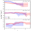 |
Fig. 11. Space density evolution as a function of redshift (z) for 1 dex luminosity bins. This is constructed with sources from M19 and M22. The 1σ bars from our RLFs are including zmax errors, Poisson errors, completeness corrections errors, and classification errors, as explained in Sects. 4.1.2 and 4.2. |
6. Discussion
With the arrival of larger FRI/FRII catalogues sensitive to lower flux densities and better redshift measurements, we have in the previous sections been able to construct RLFs up to z = 2.5 based on the M19 and M22 catalogues. We will in this section discuss the effects of energy losses on our RLFs, how the total RLAGN RLF compares to our FRI and FRII RLFs, along with the remaining selection biases, and how we can interpret the space density evolution that we find for FRIs and FRIIs.
6.1. Energy losses and the RLF
At higher redshifts, IC losses for each source become more important, as more electrons will be scattered by CMB photons when the energy density of the CMB increases. These IC losses are suggested to be one of the primary mechanisms behind the α − z relation (Klamer et al. 2006; Ghisellini et al. 2014; Morabito & Harwood 2018; Sweijen et al. 2022a), which associates steeper redshifts with higher spectral indices (Tielens et al. 1979; De Breuck et al. 2000; Miley & De Breuck 2008). Because we are interested in the redshift evolution of FRIs and FRIIs, it is important to discuss how these energy losses affect the interpretation of our RLFs.
The impact of the IC losses on the measured surface brightness of a source is mainly contingent upon the magnetic field strength within the lobes and the equivalent magnetic field associated with the CMB (Harwood et al. 2013). Due to their different morphologies, we would anticipate the IC losses to affect FRIs and FRIIs disproportionately, as this effect can alter both the size and detectability of FRIs, whereas for FRIIs the detectability will likely not change because compact hot spots at the ends of the jets are relatively unaffected. As a result, we expect that when we would take IC losses into account, the zmax and the completeness corrections will change more significant for FRIs than for FRIIs. Similarly, we could also consider other losses, such as the effects of synchrotron losses on the measured radio flux densities of FRIs and FRIIs (Myers & Spangler 1985; Alexander & Leahy 1987; Jamrozy et al. 2008; Harwood et al. 2013; Sweijen et al. 2022a). In addition, the more distant universe is also denser, which leads to a greater confinement of the radio lobes and lower adiabatic losses of sources at higher redshifts compared to sources in the local universe (e.g., Barthel & Arnaud 1996). Nevertheless, incorporating corrections for all the above mentioned energy losses would violate our initial assumption that the radio luminosity from a source remains constant as a function of redshift while calculating Vmax (see Sect. 3.2). Therefore, for the interpretation of the comparison of FRIs and FRIIs in our RLFs it is important to be aware that these are measured radio luminosity functions and not energy loss-corrected radio luminosity functions.
Fortunately, the FRI/FRII ratio RLF is less affected by those losses, as part of their effect on the zmax and completeness corrections are cancelled out. As a result, this makes the physical interpretation more comparable to the hypothetical energy-loss adjusted RLFs. The left panel of Fig. 10 supports this comparability, as the three redshift bins are the same within the uncertainties.
6.2. Comparing FRI/FRII RLFs
It is well known that FRIs and FRIIs make up a significant fraction of the total RLAGN population (Sadler 2016; Baldi et al. 2018). In this subsection, we will discuss the comparison of our FRI and FRII RLFs with those from Gendre et al. (2010, 2013) and Kondapally et al. (2022). For the total RLF we exclusively use the total RLAGN RLF from Kondapally et al. (2022), as they demonstrated consistency with previous total RLAGN RLFs in the literature.
Figure 8 shows how local the FRI space densities closely follow the total RLAGN space densities up to about L150 ∼ 1026 W Hz−1, after which FRIIs become the dominant morphology population. This similarity between the FRI and total RLAGN space densities is due to the fact that the fraction of compact sources increases towards the lower radio luminosities and we only consider sources above L150 ∼ 1024.5 W Hz−1 (e.g., Baldi et al. 2015, 2018; Capetti et al. 2020). It is reassuring to find the local RLF from Gendre et al. (2013) to be similar to ours, as this indicates that the local RLFs constructed in this paper and by Gendre et al. (2013) are not biased by the data or RLF construction methods. In Fig. 9, we observe that the space densities of the FRI and total RLAGN space densities continue to show consistent similarity up to a similar break luminosity and z = 0.8. Examination of the FRI evolution above z = 0.3 could not be accurately done by Gendre et al. (2010), due to the fact they had in their sample only seven FRIs associated with redshifts above z = 0.3 (see also Fig. 6 in Gendre et al. 2010). This is over 100 times fewer FRIs compared to what we have available from the combined M19 and M22 catalogues, comprising 877 FRIs above z = 0.3, with accurate redshifts (Duncan et al. 2019, 2021).
Beyond z = 0.8, we do not find a well-defined break luminosity above which FRIIs dominate over FRIs. However, we do find in Fig. 9 above L150 ∼ 1026 W Hz−1 the FRIIs to be a dominant morphology type when we compare the total RLAGN space densities with the FRII space densities. This demonstrates that up to z = 2.5, the FRIIs dominate the RLAGN population at the high radio luminosity end. Below L150 ∼ 1026 W Hz−1 and beyond z = 0.8 we detect a prominent offset in the order of 1–1.5 dex between the total RLAGN and the FRI and FRII space densities. This is likely related to remaining unaccounted selection effects. Some of this might be a result of energy loss effects that we did not take into account, which more strongly affect FRI detections (see Sect. 6.1). Also the probable underestimation of the completeness corrections for FRIs due to the difficulty to accurately measure their sizes in the higher redshift bins could play a role (see Sect. 4.2.2). Moreover, Kondapally et al. (2022) discusse how the space densities of star-forming low-excitation radio galaxies (LERGs) increase over redshift and dominate the LERG space densities after z ∼ 1, while the space densities of quiescent LERGs decreases over redshift. Given that low-power FRIs and FRIIs are predominantly associated with LERGs (Mingo et al. 2022), there is a possible selection bias in our completeness corrections that is unaccounted for if some of those star-forming LERGs might indeed turn out to be FRIs or FRIIs with small jets that are difficult to detect at a resolution of 6″. We also argue that the difficulty to detect star-forming radio galaxies with radio jets in our sample is likely a more significant issue for FRIs, as their smaller weaker jets are more difficult to detect compared to FRIIs. Other missing morphology types such as hybrid or double–double sources are expected to be rare (Harwood et al. 2020; Mingo et al. 2019, 2022) and therefore will not have a significant contribution to remaining selection effects. Thus, although the redshift simulations help us to correct for observational biases when deriving zmax values (see Sect. 4.1.1) and completeness corrections (see Sect. 4.2.1), it is possible that residual resolution and surface brightness limits could still reside in selection effects that we are not yet able to fully correct for.
6.3. Space density enhancements
Space density enhancements of the total RLAGN RLF have been well-measured for a long time (e.g., Dunlop & Peacock 1990). Multiple studies have found space density enhancements for bright FRIs and FRIIs (Snellen & Best 2001; Willott et al. 2001; Jamrozy 2004; Rigby et al. 2008; Gendre et al. 2010). Given our increased number of sources above z = 0.3 compared to previous studies, it is valuable to re-examine the space density enhancements and declines with our RLFs and look specifically how these relate to our understanding of radio galaxy evolution.
The space density enhancement from low to high redshift that we find for FRIs and FRIIs above L150 ∼ 1027 W Hz−1 could simply be related to the higher gas availability in the earlier universe, increasing the probability for RLAGN to become more powerful. Although taking into account energy loss effects in our RLFs is complex and beyond the scope of this paper (see Sect. 6.1), it is worth mentioning that if the net energy loss effects are lower in the earlier denser universe (e.g., significant lower adiabatic losses) compared to the local universe, we could expect to measure even more powerful sources at higher redshifts. We are not well-enough constrained for bright FRIs to find a notable difference between the space density enhancements of FRIs and FRIIs above L150 ∼ 1027 W Hz−1 (see Figs. 10 and 11). Nevertheless, a recent simulation demonstrated how radio sources were more likely to live in less rich environments at z = 2 compared to z = 0 (Thomas & Davé 2022), which is in favor of FRII morphologies (Croston et al. 2019). More data at the high radio luminosity end would help to better constrain the FRI and FRII space density enhancements and test if powerful FRIIs have indeed a stronger space density enhancement than powerful FRIs.
The space density decline of FRIs below L150 ∼ 1026 W Hz−1 is likely related to unaccounted selection effects, as we discussed in Sect. 6.2 to explain the observed space density offsets between the local and higher redshift bins. However, despite the fact that the remaining selection effects have a stronger effect on the space densities from FRIs than FRIIs, we find the FRI/FRII space density ratio over all radio luminosities to be remarkably similar when we compare the three redshift bins in the left panel of Fig. 10. If this holds for larger and more comprehensive sample sizes, resulting in reduced Poisson errors, it could suggest that the jet-disruption of FRIs is not primarily influenced by environmental factors, as those evolve over redshift. Instead, disruption of the jets from the FRI parent population would more likely be associated with events happening in close proximity to, or within, the parent radio galaxy.
6.4. Future prospects
We demonstrate in this paper how detection limits are affecting selection biases and how it is possible to partly correct for these if we want to construct reliable RLFs from RLAGN. In order to enhance the significance of our findings, we need more objects from more sensitive radio maps along with wider area observations. The 40″ angular size cut that we needed to apply, due to the angular size selection from Mingo et al. (2019), removes a large fraction of the small FRIs and FRIIs. Especially sources at the lowest radio flux densities are the most affected. The angular size cut is due to the 6″ resolution from the LoTSS radio maps that were used to extract the FRI and FRII sources from. So, to collect a reliable sample below 40″, we need to improve the resolution.
Recent efforts have been ongoing to increase the sky coverage with LoTSS DR2 at 6″ (Shimwell et al. 2022), which will increase the number of objects in M19 by a factor of about 13. This data release is based on radio maps at the same resolution and a similar sensitivity as LoTSS DR1. This will therefore only help to reduce the uncertainties at the higher radio luminosity end and up to z = 0.8. Fortunately, work has also been done to bring LOFAR’s resolution down to 0.3″ by including all baselines up to ∼2000 km (Varenius et al. 2015, 2016; Harris et al. 2019; Morabito et al. 2022; Sweijen et al. 2022b). This resolution will help us to collect sources that are unresolved at 6″, such that we can lower the 40″ angular size cut. An improved resolution comes with the unavoidable loss of surface brightness sensitivity. Sweijen et al. (2022b) reported from 6″ to 0.3″ an estimated 60% detection loss of sources that were unresolved at 6″. As FRIs are on average less bright and have by definition diffuser jets than FRIIs, this will surely have a more negative effect on the detections of FRIs compared to FRIIs. To ensure that enough small FRIs will be detected, it becomes essential to improve the sensitivity by processing and calibrating multiple observations of the same fields (de Jong et al., in prep.) and to complement these high resolution radio maps with intermediate resolutions around for example ∼1″ (Ye et al. 2023).
7. Conclusions
We presented in this paper RLFs of FRI and FRII morphologies up to z = 2.5 and beyond L150 ∼ 1024.5 W Hz−1, by utilizing the M19 and M22 catalogues. We corrected for redshift effects and the incompleteness of our sample by using the redshifting algorithm. This algorithm gave us a reliable estimate of the maximum distance an FRI and FRII source can still be classified. In particular, our RLFs for FRIs are an improvement above z = 0.3, as we have over 100 times more available FRIs with associated redshifts above this redshift, compared to previous studies (Gendre et al. 2010, 2013). These RLFs also provide us with continuing evidence of evolution of FRI and FRII sources.
In our RLFs, we do not detect any sharp transitions between the FRI and FRII morphologies as a function of radio luminosity or redshift. We find a space density enhancement from low to high redshift for FRI and FRII sources beyond L150 ∼ 1027 W Hz−1, which might be explained by a higher gas availability in the earlier universe, increasing the likelihood for FRIs and FRIIs to become powerful. Also, the net energy losses at higher redshifts could potentially increase the measured radio luminosities at higher redshifts if the adiabatic losses are significantly lower compared to lower redshifts. However, to test this assertion we need a more detailed analysis of the different energy loss effects (e.g., IC and synchrotron losses), which is beyond the scope of this paper. At the low radio luminosity end, we tentatively identify a declining trend of the FRI space densities with redshift. This is likely related to remaining selection effects such as from the underestimation of distant FRI angular sizes at higher redshifts and the difficulty to detect star-forming FRIs with small jets, which have been proven to be more prominent at higher redshifts. Although there are significant uncertainties represented by the large error bars, the evolution of the FRI/FRII ratio that we derive suggests that the FRI morphology is primarily a result of the disruption of jets on scales originating within or close to the host galaxy, rather than jet-disruption due to large-scale environmental factors.
The potential residual selection biases in our results highlight the necessity to further develop the calibration and imaging pipeline of LOFAR data with baselines up to 2000 km, such that it will be possible to incorporate radio sources at smaller angular scales and lower radio luminosities. This will eventually help to more precisely model the FRI and FRII sources above z = 0.3 towards lower radio luminosities, which can further enhance our understanding of radio jet evolution from RLAGN and the link between these jets and their environment and host galaxies.
See also the LOFAR Galaxy Zoo project: https://www.zooniverse.org/projects/chrismrp/radio-galaxy-zoo-lofar
Acknowledgments
This publication is part of the project CORTEX (NWA.1160.18.316) of the research programme NWA-ORC which is (partly) financed by the Dutch Research Council (NWO). This work made use of the Dutch national e-infrastructure with the support of the SURF Cooperative using grant no. EINF-1287. R.K. and P.N.B. are grateful for support from the UK STFC via grant ST/V000594/1. B.M. acknowledges support from the Science and Technology Facilities Council (STFC) under grants ST/T000295/1 and ST/X001164/1. R.J.v.W. acknowledges support from the ERC Starting Grant ClusterWeb 804208. This work was supported by the Medical Research Council [MR/T042842/1]. LOFAR data products were provided by the LOFAR Surveys Key Science project (LSKSP; https://lofar-surveys.org/) and were derived from observations with the International LOFAR Telescope (ILT). LOFAR (van Haarlem et al. 2013) is the Low Frequency Array designed and constructed by ASTRON. It has observing, data processing, and data storage facilities in several countries, which are owned by various parties (each with their own funding sources), and which are collectively operated by the ILT foundation under a joint scientific policy. The efforts of the LSKSP have benefited from funding from the European Research Council, NOVA, NWO, CNRS-INSU, the SURF Co-operative, the UK Science and Technology Funding Council and the Jülich Supercomputing Centre. For the purpose of open access, the author has applied a Creative Commons Attribution (CC BY) licence to any Author Accepted Manuscript version.
References
- Alexander, P., & Leahy, J. P. 1987, MNRAS, 225, 1 [NASA ADS] [CrossRef] [Google Scholar]
- Baldi, R. D., Capetti, A., & Giovannini, G. 2015, A&A, 576, A38 [NASA ADS] [CrossRef] [EDP Sciences] [Google Scholar]
- Baldi, R. D., Capetti, A., & Massaro, F. 2018, A&A, 609, A1 [NASA ADS] [CrossRef] [EDP Sciences] [Google Scholar]
- Banfield, J. K., Wong, O. I., Willett, K. W., et al. 2015, MNRAS, 453, 2326 [Google Scholar]
- Barišić, I., van der Wel, A., van Houdt, J., et al. 2019, ApJ, 872, L12 [CrossRef] [Google Scholar]
- Barthel, P. D., & Arnaud, K. A. 1996, MNRAS, 283, L45 [NASA ADS] [CrossRef] [Google Scholar]
- Best, P. N. 2009, Astron. Nachr., 330, 184 [NASA ADS] [CrossRef] [Google Scholar]
- Best, P. N., Kaiser, C. R., Heckman, T. M., & Kauffmann, G. 2006, MNRAS, 368, L67 [NASA ADS] [Google Scholar]
- Best, P. N., Kondapally, R., Williams, W. L., et al. 2023, MNRAS, 523, 1729 [NASA ADS] [CrossRef] [Google Scholar]
- Bicknell, G. V. 1995, ApJS, 101, 29 [Google Scholar]
- Blandford, R., Meier, D., & Readhead, A. 2019, ARA&A, 57, 467 [NASA ADS] [CrossRef] [Google Scholar]
- Calistro Rivera, G., Williams, W. L., Hardcastle, M. J., et al. 2017, MNRAS, 469, 3468 [Google Scholar]
- Capetti, A., Massaro, F., & Baldi, R. D. 2017a, A&A, 598, A49 [NASA ADS] [CrossRef] [EDP Sciences] [Google Scholar]
- Capetti, A., Massaro, F., & Baldi, R. D. 2017b, A&A, 601, A81 [NASA ADS] [CrossRef] [EDP Sciences] [Google Scholar]
- Capetti, A., Brienza, M., Baldi, R. D., et al. 2020, A&A, 642, A107 [NASA ADS] [CrossRef] [EDP Sciences] [Google Scholar]
- Cattaneo, A., Faber, S. M., Binney, J., et al. 2009, Nature, 460, 213 [NASA ADS] [CrossRef] [Google Scholar]
- Cochrane, R. K., Kondapally, R., Best, P. N., et al. 2023, MNRAS, 523, 6082 [NASA ADS] [CrossRef] [Google Scholar]
- Condon, J. J., Cotton, W. D., & Broderick, J. J. 2002, AJ, 124, 675 [Google Scholar]
- Croton, D. J., Springel, V., White, S. D. M., et al. 2006, MNRAS, 365, 11 [Google Scholar]
- Croston, J. H., Hardcastle, M. J., Mingo, B., et al. 2019, A&A, 622, A10 [NASA ADS] [CrossRef] [EDP Sciences] [Google Scholar]
- De Breuck, C., van Breugel, W., Röttgering, H. J. A., & Miley, G. 2000, A&AS, 143, 303 [NASA ADS] [CrossRef] [EDP Sciences] [Google Scholar]
- DeForest, C. E. 2004, Sol. Phys., 219, 3 [NASA ADS] [CrossRef] [Google Scholar]
- Duncan, K. J., Sabater, J., Röttgering, H. J. A., et al. 2019, A&A, 622, A3 [NASA ADS] [CrossRef] [EDP Sciences] [Google Scholar]
- Duncan, K. J., Kondapally, R., Brown, M. J. I., et al. 2021, A&A, 648, A4 [EDP Sciences] [Google Scholar]
- Dunlop, J. S., & Peacock, J. A. 1990, MNRAS, 247, 19 [NASA ADS] [Google Scholar]
- Fabian, A. C. 2012, ARA&A, 50, 455 [Google Scholar]
- Fanaroff, B. L., & Riley, J. M. 1974, MNRAS, 167, 31 [Google Scholar]
- Gehrels, N. 1986, ApJ, 303, 336 [Google Scholar]
- Gendre, M. A., & Wall, J. V. 2008, MNRAS, 390, 819 [NASA ADS] [Google Scholar]
- Gendre, M. A., Best, P. N., & Wall, J. V. 2010, MNRAS, 404, 1719 [Google Scholar]
- Gendre, M. A., Best, P. N., Wall, J. V., & Ker, L. M. 2013, MNRAS, 430, 3086 [NASA ADS] [CrossRef] [Google Scholar]
- Ghisellini, G., Celotti, A., Tavecchio, F., Haardt, F., & Sbarrato, T. 2014, MNRAS, 438, 2694 [NASA ADS] [CrossRef] [Google Scholar]
- Gopal-Krishna, & Wiita, P. J. 2000, A&A, 363, 507 [Google Scholar]
- Hales, C. A., Norris, R. P., Gaensler, B. M., et al. 2014, MNRAS, 441, 2555 [Google Scholar]
- Hardcastle, M. J., & Croston, J. H. 2020, New Astron. Rev., 88, 101539 [Google Scholar]
- Hardcastle, M. J., Gürkan, G., van Weeren, R. J., et al. 2016, MNRAS, 462, 1910 [Google Scholar]
- Hardcastle, M. J., Williams, W. L., Best, P. N., et al. 2019, A&A, 622, A12 [NASA ADS] [CrossRef] [EDP Sciences] [Google Scholar]
- Harris, D. E., Moldón, J., Oonk, J. R. R., et al. 2019, ApJ, 873, 21 [Google Scholar]
- Harwood, J. J., Hardcastle, M. J., Croston, J. H., & Goodger, J. L. 2013, MNRAS, 435, 3353 [NASA ADS] [CrossRef] [Google Scholar]
- Harwood, J. J., Vernstrom, T., & Stroe, A. 2020, MNRAS, 491, 803 [Google Scholar]
- Huynh, M. T., Jackson, C. A., Norris, R. P., & Prandoni, I. 2005, AJ, 130, 1373 [Google Scholar]
- Jackson, C. A., & Wall, J. V. 1999, MNRAS, 304, 160 [NASA ADS] [CrossRef] [Google Scholar]
- Jamrozy, M. 2004, A&A, 419, 63 [NASA ADS] [CrossRef] [EDP Sciences] [Google Scholar]
- Jamrozy, M., Konar, C., Machalski, J., & Saikia, D. J. 2008, MNRAS, 385, 1286 [NASA ADS] [CrossRef] [Google Scholar]
- Jannuzi, B. T., & Dey, A. 1999, ASP Conf. Ser., 193, 258 [Google Scholar]
- Kaiser, C. R., & Best, P. N. 2007, MNRAS, 381, 1548 [Google Scholar]
- Kauffmann, G., Heckman, T. M., Tremonti, C., et al. 2003, MNRAS, 346, 1055 [Google Scholar]
- Klamer, I. J., Ekers, R. D., Bryant, J. J., et al. 2006, MNRAS, 371, 852 [Google Scholar]
- Kondapally, R., Best, P. N., Hardcastle, M. J., et al. 2021, A&A, 648, A3 [EDP Sciences] [Google Scholar]
- Kondapally, R., Best, P. N., Cochrane, R. K., et al. 2022, MNRAS, 513, 3742 [NASA ADS] [CrossRef] [Google Scholar]
- Kormendy, J., & Ho, L. C. 2013, ARA&A, 51, 511 [Google Scholar]
- Krolik, J. H., & Chen, W. 1991, AJ, 102, 1659 [NASA ADS] [CrossRef] [Google Scholar]
- Ledlow, M. J., & Owen, F. N. 1996, AJ, 112, 9 [Google Scholar]
- Lockman, F. J., Jahoda, K., & McCammon, D. 1986, ApJ, 302, 432 [Google Scholar]
- Lynden-Bell, D. 1969, Nature, 223, 690 [NASA ADS] [CrossRef] [Google Scholar]
- Magliocchetti, M. 2022, A&A Rev, 30, 6 [NASA ADS] [CrossRef] [Google Scholar]
- Magorrian, J., Tremaine, S., Richstone, D., et al. 1998, AJ, 115, 2285 [Google Scholar]
- Mahony, E. K., Morganti, R., Prandoni, I., et al. 2016, MNRAS, 463, 2997 [Google Scholar]
- Mandal, S., Prandoni, I., Hardcastle, M. J., et al. 2021, A&A, 648, A5 [EDP Sciences] [Google Scholar]
- Martini, P., Miller, E. D., Brodwin, M., et al. 2013, ApJ, 768, 1 [Google Scholar]
- Mauch, T., & Sadler, E. M. 2007, MNRAS, 375, 931 [Google Scholar]
- McNamara, B. R., & Nulsen, P. E. J. 2007, ARA&A, 45, 117 [NASA ADS] [CrossRef] [Google Scholar]
- Miley, G., & De Breuck, C. 2008, A&A Rev, 15, 67 [NASA ADS] [CrossRef] [Google Scholar]
- Mingo, B., Croston, J. H., Hardcastle, M. J., et al. 2019, MNRAS, 488, 2701 [NASA ADS] [CrossRef] [Google Scholar]
- Mingo, B., Croston, J. H., Best, P. N., et al. 2022, MNRAS, 511, 3250 [NASA ADS] [CrossRef] [Google Scholar]
- Morabito, L. K., & Harwood, J. J. 2018, MNRAS, 480, 2726 [Google Scholar]
- Morabito, L. K., Jackson, N. J., Mooney, S., et al. 2022, A&A, 658, A1 [NASA ADS] [CrossRef] [EDP Sciences] [Google Scholar]
- Morganti, R. 2017, Front. Astron. Space Sci., 4, 42 [CrossRef] [Google Scholar]
- Mostert, R. I. J., Duncan, K. J., Alegre, L., et al. 2022, A&A, 668, A28 [NASA ADS] [CrossRef] [EDP Sciences] [Google Scholar]
- Murphy, E. J., Momjian, E., Condon, J. J., et al. 2017, ApJ, 839, 35 [Google Scholar]
- Myers, S. T., & Spangler, S. R. 1985, ApJ, 291, 52 [NASA ADS] [CrossRef] [Google Scholar]
- O’Dea, C. P., & Saikia, D. J. 2021, A&A Rev, 29, 3 [CrossRef] [Google Scholar]
- Oei, M. S. S. L., van Weeren, R. J., Gast, A. R. D. J. G. I. B., et al. 2023, A&A, 672, A163 [NASA ADS] [CrossRef] [EDP Sciences] [Google Scholar]
- Oliver, S., Rowan-Robinson, M., Alexander, D. M., et al. 2000, MNRAS, 316, 749 [Google Scholar]
- Owen, F. N., & Rudnick, L. 1976, ApJ, 205, L1 [NASA ADS] [CrossRef] [Google Scholar]
- Padovani, P. 2016, A&A Rev, 24, 13 [NASA ADS] [CrossRef] [Google Scholar]
- Parma, P., de Ruiter, H. R., & Fanti, R. 1996, in Extragalactic Radio Sources, eds. R. D. Ekers, C. Fanti, & L. Padrielli, 175, 137 [NASA ADS] [CrossRef] [Google Scholar]
- Prandoni, I., Gregorini, L., Parma, P., et al. 2001, A&A, 365, 392 [NASA ADS] [CrossRef] [EDP Sciences] [Google Scholar]
- Prandoni, I., Guglielmino, G., Morganti, R., et al. 2018, MNRAS, 481, 4548 [Google Scholar]
- Prescott, M., Mauch, T., Jarvis, M. J., et al. 2016, MNRAS, 457, 730 [Google Scholar]
- Retana-Montenegro, E., Röttgering, H. J. A., Shimwell, T. W., et al. 2018, A&A, 620, A74 [NASA ADS] [CrossRef] [EDP Sciences] [Google Scholar]
- Rigby, E. E., Best, P. N., & Snellen, I. A. G. 2008, MNRAS, 385, 310 [NASA ADS] [CrossRef] [Google Scholar]
- Sabater, J., Best, P. N., Hardcastle, M. J., et al. 2019, A&A, 622, A17 [NASA ADS] [CrossRef] [EDP Sciences] [Google Scholar]
- Sabater, J., Best, P. N., Tasse, C., et al. 2021, A&A, 648, A2 [EDP Sciences] [Google Scholar]
- Sadler, E. M. 2016, Astron. Nachr., 337, 105 [Google Scholar]
- Schmidt, M. 1968, ApJ, 151, 393 [Google Scholar]
- Schoenmakers, A. P., de Bruyn, A. G., Röttgering, H. J. A., & van der Laan, H. 2000, MNRAS, 315, 395 [NASA ADS] [CrossRef] [Google Scholar]
- Shimwell, T. W., Röttgering, H. J. A., Best, P. N., et al. 2017, A&A, 598, A104 [NASA ADS] [CrossRef] [EDP Sciences] [Google Scholar]
- Shimwell, T. W., Tasse, C., Hardcastle, M. J., et al. 2019, A&A, 622, A1 [NASA ADS] [CrossRef] [EDP Sciences] [Google Scholar]
- Shimwell, T. W., Hardcastle, M. J., Tasse, C., et al. 2022, A&A, 659, A1 [NASA ADS] [CrossRef] [EDP Sciences] [Google Scholar]
- Singal, A. K., & Rajpurohit, K. 2014, MNRAS, 442, 1656 [NASA ADS] [CrossRef] [Google Scholar]
- Snellen, I. A. G., & Best, P. N. 2001, MNRAS, 328, 897 [NASA ADS] [CrossRef] [Google Scholar]
- Sweijen, F., Morabito, L. K., Harwood, J., et al. 2022a, A&A, 658, A3 [NASA ADS] [CrossRef] [EDP Sciences] [Google Scholar]
- Sweijen, F., van Weeren, R. J., Röttgering, H. J. A., et al. 2022b, Nat. Astron., 6, 350 [NASA ADS] [CrossRef] [Google Scholar]
- Tasse, C., Shimwell, T., Hardcastle, M. J., et al. 2021, A&A, 648, A1 [EDP Sciences] [Google Scholar]
- Thomas, N., & Davé, R. 2022, MNRAS, 515, 5539 [NASA ADS] [CrossRef] [Google Scholar]
- Tielens, A. G. G. M., Miley, G. K., & Willis, A. G. 1979, A&AS, 35, 153 [NASA ADS] [Google Scholar]
- van Haarlem, M. P., Wise, M. W., Gunst, A. W., et al. 2013, A&A, 556, A2 [NASA ADS] [CrossRef] [EDP Sciences] [Google Scholar]
- Varenius, E., Conway, J. E., Martí-Vidal, I., et al. 2015, A&A, 574, A114 [NASA ADS] [CrossRef] [EDP Sciences] [Google Scholar]
- Varenius, E., Conway, J. E., Martí-Vidal, I., et al. 2016, A&A, 593, A86 [NASA ADS] [CrossRef] [EDP Sciences] [Google Scholar]
- Williams, W. L., van Weeren, R. J., Röttgering, H. J. A., et al. 2016, MNRAS, 460, 2385 [Google Scholar]
- Williams, W. L., Hardcastle, M. J., Best, P. N., et al. 2019, A&A, 622, A2 [NASA ADS] [CrossRef] [EDP Sciences] [Google Scholar]
- Willott, C. J., Rawlings, S., Blundell, K. M., Lacy, M., & Eales, S. A. 2001, MNRAS, 322, 536 [NASA ADS] [CrossRef] [Google Scholar]
- Windhorst, R., Mathis, D., & Neuschaefer, L. 1990, ASP Conf. Ser., 10, 389 [Google Scholar]
- Wing, J. D., & Blanton, E. L. 2011, AJ, 141, 88 [CrossRef] [Google Scholar]
- Ye, H., Sweijen, F., van Weeren, R., et al. 2023, A&A, submitted [arXiv:2309.16560] [Google Scholar]
- Zheng, X. C., Röttgering, H. J. A., Best, P. N., et al. 2020, A&A, 644, A12 [NASA ADS] [CrossRef] [EDP Sciences] [Google Scholar]
- Zheng, X. C., Röttgering, H. J. A., van der Wel, A., & Duncan, K. 2022, A&A, 665, A114 [NASA ADS] [CrossRef] [EDP Sciences] [Google Scholar]
Appendix A: Testing the RLF reliability
Relocating sources to higher redshifts reduces their flux densities and apparent sizes, which makes it more difficult to detect and classify FRI and FRII sources. Figure 5 shows how FRIs and FRIIs are affected differently by these effects. To test whether the Vmax method and our completeness corrections are taking the effect, due to changes in flux density and resolution, correctly into account, we compare an FRI and FRII sample below z < 0.4 with the same sample shifted to z = 1.5. This is done by using the algorithm from Section 3.2 and applying the same completeness correction process discussed in Section 4.2. If our Vmax method and completeness corrections are well-applied, we expect the derived space densities of the original z < 0.4 sample and of the same sample shifted to 1.5 < z < 2.5 to agree with each other, as the simulated sample has larger space density corrections and smaller Vmax values. The left panel from Figure A.1 has a sample of 478 FRIs before relocating them to z = 1.5. After relocating there are only 105 sources that could be classified. Although the number reduces with a factor 4, we find that the radio luminosity functions to still agree with each other. In the right panel of this same figure we also compare the RLF ratios before and after relocating and also find a strong agreement. We have also experimented with other redshift bins (smaller and larger) and find similar agreements. This gives us additional confidence that both the Vmax and the completeness corrections are applied well.
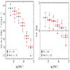 |
Fig. A.1. RLF space density evolution difference between the original and simulated sample. Left: RLF for FRI sample before and after applying the redshifting algorithm from z < 0.4 to z = 1.5. Right: RLF ratio for a sample of FRI and FRII sources before and after applying the redshifting algorithm from z < 0.4 to z = 1.5. Error bars from our RLFs are including zmax errors, Poisson errors, completeness corrections errors, and classification errors. |
To test the completeness corrections derived with the angular size distribution (see Section 4.2), we applied a larger angular size cut at 80″ and compared the space densities with the already present 40″ cut. The comparison for sources below z = 0.5 is shown in Figure A.2 and shows how (even though the number count is reduced by nearly a factor of 2) the completeness corrections correct remarkably well for this effect and make the both RLFs agree with each other. We also compared this for other angular size cuts and found similar consistencies. This demonstrates the reliability to correct our space densities with the angular size distributions from Windhorst et al. (1990) with updated fitting parameters from Mandal et al. (2021) on a local sample.
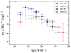 |
Fig. A.2. Comparison between a 40″ and 80″ source cut below z = 0.5. Both RLFs are corrected with the completeness corrections from Section 4.2. The angular size completeness correction is applied for respectively the 40″ and 80″ angular sizes. This figure contains all sources in the redshift bin 0 < z < 1.0. The 40″ cut selection has 865 sources, while the 80″ cut has 405 sources left. The 1σ error bars are containing zmax errors, Poisson errors, completeness corrections errors, and classification errors. |
All Tables
All Figures
|
Fig. 1. Angular size as a function of flux density (left panel) and redshift (right panel) for the 1560 sources considered in this paper. We separated our sources into 1146 FRI and 414 FRII morphologies with separated colors and draw dashed lines for 40″ and 400″. These lines determine the angular size cuts that we applied in this paper before doing completeness corrections (see Sect. 4.2). |
| In the text | |
|
Fig. 2. Luminosity–redshift diagram for M19 and M22 split in FRIs and FRIIs. |
| In the text | |
|
Fig. 3. Examples of FRI sources after redshift increments by applying the redshifting algorithm. All unassociated emission is masked out (in this case below 4σ). Each columns displays the source from the same row at different redshifts. The last row is a wide-angle tail FRI source (Owen & Rudnick 1976), where after redshift increments, the source appears to resemble an FRII source. The optical host location is in every image given by the green cross. (a) FRI at z = 0.48, (b) FRI at z = 0.93, (c) FRI at z = 1.38, (d) FRI at z = 0.19, (e) FRI at z = 0.39, (f) FRI at z = 0.59, (g) FRI at z = 0.29, (h) FRI at z = 0.69, (i) FRI at z = 1.19. |
| In the text | |
|
Fig. 4. Examples of FRII sources after redshift increments by applying the redshifting algorithm. All unassociated emission is masked out (in this case below 4σ). Each column displays the source from the same row at different redshifts. The optical host location is in every image given by the green cross. (a) FRII at z = 0.33, (b) FRII at z = 0.83, (c) FRII at z = 1.33, (d) FRII at z = 0.9, (e) FRII at z = 1.5, (f) FRII at z = 2.1, (g) FRII at z = 0.34, (h) FRII at z = 1.34, (i) FRII at z = 1.84. |
| In the text | |
|
Fig. 5. Fraction of local (z < 0.5) FRI and FRII sources that are still classifiable after applying redshift increments with the redshifting algorithm as a function of redshift. The error bars include the errors on zmax and Poisson errors. |
| In the text | |
|
Fig. 6. Luminosity versus redshift increments with the redshifting algorithm for 150 random sources at different luminosities from all sources from M19 and M22 above L150 ∼ 1022 W Hz−1. The starting positions are at the original measured redshifts given by the squared boxes, while the ending positions are the final maximum redshifts a source can be classified (up to z = 2.5). |
| In the text | |
|
Fig. 7. Completeness corrections for FRI and FRII sources from M19 and M22. |
| In the text | |
|
Fig. 8. Local RLF for FRIs and FRIIs from this paper are plotted in blue and red, respectively. For comparison and to validate that our FRI and FRII space densities do not extend above the total RLAGN population, we added the total local RLAGN RLF from Kondapally et al. (2022) beyond L150 ∼ 1024 W Hz−1 (in green). This total RLAGN RLF is constructed based on sources from the LoTSS-Deep Fields DR1. To demonstrate that our results agree with previous work, we also added the FRI and FRII RLF from Gendre et al. (2013) in black and orange, respectively. These points are based on the CoNFIG catalogue (Gendre & Wall 2008; Gendre et al. 2010), where we converted the luminosity bins to 150 MHz by using a spectral index of α = 0.7. The 1σ bars from our RLFs are including zmax errors, Poisson errors, completeness corrections errors, and classification errors. All our data points are given in Table 2. |
| In the text | |
|
Fig. 9. RLF for FRI (blue) and FRII (red) sources split in different redshift bins. For comparison and to show that our FRI and FRII space densities do not extend above the total RLAGN population, we added the total RLAGN RLF from Kondapally et al. (2022) beyond L150 ∼ 1024 W Hz−1 in green. We also added the local RLFs for both FRIs and FRIIs with dot-dashed lines. We removed radio luminosity bins which only contain a single source. The 1σ bars from our RLFs are including zmax errors, Poisson errors, completeness corrections errors, and classification errors, as explained in Sects. 4.1.2 and 4.2. Data points are given in Table 2. |
| In the text | |
|
Fig. 10. RLF ratio evolution. Left: ratio evolution over different redshift bins. Right: separated FRI (above) and FRII (below) space density evolution plots corresponding to the ratio evolution plot in the left panel. In both figures, we added the Gendre et al. (2013) data points for the higher end of the luminosity range, such that we can further constrain the local RLF, which was fitted with a broken power law from Eq. (8) and corresponding values from Table 1, where we used a 1σ confidence interval. We removed radio luminosity bins which only contain a single source. The 1σ bars from our RLFs are including zmax errors, Poisson errors, completeness corrections errors, and classification errors, as explained in Sects. 4.1.2 and 4.2. |
| In the text | |
|
Fig. 11. Space density evolution as a function of redshift (z) for 1 dex luminosity bins. This is constructed with sources from M19 and M22. The 1σ bars from our RLFs are including zmax errors, Poisson errors, completeness corrections errors, and classification errors, as explained in Sects. 4.1.2 and 4.2. |
| In the text | |
|
Fig. A.1. RLF space density evolution difference between the original and simulated sample. Left: RLF for FRI sample before and after applying the redshifting algorithm from z < 0.4 to z = 1.5. Right: RLF ratio for a sample of FRI and FRII sources before and after applying the redshifting algorithm from z < 0.4 to z = 1.5. Error bars from our RLFs are including zmax errors, Poisson errors, completeness corrections errors, and classification errors. |
| In the text | |
|
Fig. A.2. Comparison between a 40″ and 80″ source cut below z = 0.5. Both RLFs are corrected with the completeness corrections from Section 4.2. The angular size completeness correction is applied for respectively the 40″ and 80″ angular sizes. This figure contains all sources in the redshift bin 0 < z < 1.0. The 40″ cut selection has 865 sources, while the 80″ cut has 405 sources left. The 1σ error bars are containing zmax errors, Poisson errors, completeness corrections errors, and classification errors. |
| In the text | |
Current usage metrics show cumulative count of Article Views (full-text article views including HTML views, PDF and ePub downloads, according to the available data) and Abstracts Views on Vision4Press platform.
Data correspond to usage on the plateform after 2015. The current usage metrics is available 48-96 hours after online publication and is updated daily on week days.
Initial download of the metrics may take a while.