© The Authors 2023

1 Introduction

A database intended for the modeling of cometary comas and planetary atmospheres was recently reported that includes thermally averaged cross sections (TACS) for rotational state-to-state transitions in H₂O + H₂O collisions (Mandal & Babikov 2023). The database contains 231 transitions between para-states and 210 transitions between ortho-states of a “target” water molecule (for H₂O states at energies below E = 700 cm⁻¹, up to j = 7), obtained assuming thermal distribution of the rotational states of “collider” water molecules in the temperature range between 150 K and 800 K. It is also assumed that cross sections σ from that database can be easily converted into the corresponding rate coefficients using k(T) = υ_ave(T) × σ(U), where ${\upsilon }_{\text{ave}}\left(T\right)=\sqrt{\left(8k_{\text{B}}T/\mu \pi \right)}$ is the average collision velocity at a given temperature, µ is the reduced mass of collision partners, and U = (4/π)k_BT is kinetic energy, which corresponds to the average collision velocity.

However, it should be understood that this simple method of computing rate coefficients is approximate, because it assumes that one value of collision energy U can represent thermal distribution, which is equivalent to assuming that cross section σ is independent of U. Although it was used in the recent literature (Boursier et al. 2020; Buffa et al. 2000), this method is expected to be valid only for a short range of intermediate temperatures. Indeed, it may break down at lower temperatures because at low collision energies the energy dependence of cross section σ(U) is usually sharper. It may also break down at higher temperatures when the energy distribution is broader, with no one representative value of U.

The rigorous expression for calculation of the rate coefficient includes averaging over the thermal distribution of collision energies (for n → n′ quenching process): $$k_{n\to n^{\prime }}\left(T\right)=\frac{{\upsilon }_{\text{ave}}\left(T\right)}{{\left(k_{\text{B}}T\right)}^2}{\displaystyle \underset{E=0}{\overset{\infty }{\int }}E{\sigma }_{n\to n^{\prime }}\left(E\right){\text{e}}^{-\frac{E}{k_{\text{B}}T}}\text{d}E,}$$(1)

where σ_n→n′(E) is the actual dependence of the inelastic cross section on the kinetic energy of the collision (Żółtowski et al. 2022), with n being used as a composite index for labeling the rotational states of the molecule (i.e., with n representing $j_{k_{\text{a}}{k}_{\text{c}}}$ states of asymmetric-top rotor molecules such as H₂O). The first, applied goal of this paper, is to employ formulae such as Eq. (1), which improves the overall prediction of the temperature dependence of rate coefficients but also allows expansion of the range of temperatures towards the low-T regime. This is particularly important for the modeling of cometary environments (Bockelée-Morvan et al. 2010; Cochran et al. 2015; Dones et al. 2015; Cordiner et al. 2020) or the atmospheres of icy planets (Hartogh et al. 2011; Vorburger et al. 2022; Wirström et al. 2020), where temperatures below 150 K are typical. Expansion of the H₂O + H₂O database into the low-T range is achieved here by interpolation between the reference data (Mandal & Babikov 2023) and the process threshold, where the kinetic energy is barely enough for the excitation process n′→n, and therefore the excitation cross section σ_n′→n(E) is known to vanish. We note that the atmospheres of Ganymede, Calisto, and Europa will be investigated in detail by the ESA Jupiter Icy Moons Explorer mission (JUICE), which focuses on rotational transitions in water at high resolution (Bruzzone et al. 2013; Enya et al. 2022; Vorburger et al. 2022). Moreover, in cometary comas, nonequi-librium conditions occur between the inner (collision-controlled) and the outermost (fluorescence-controlled) parts of the expanding gas (Bonev et al. 2021; Cochran et al. 2015; Cordiner et al. 2022; Roth et al. 2021). Interpretation of these and many other observations requires numerical modeling with radiation transfer codes, which, in turn, requires collision rate coefficients for H₂O + H₂O as input. Large errors on these rate coefficients can affect the predictions of astrophysical modeling by orders of magnitude (Al-Edhari et al. 2017; Faure & Josselin 2008; Faure et al. 2018; Khalifa et al. 2020).

The second, more methodological goal of this paper is to offer a general method for the calculations of rate coefficients that satisfy the principle of microscopic reversibility: $$w_n{k}_{n\to n^{\prime }}=w_{n^{\prime }}{k}_{n^{\prime }\to n}.$$(2)

Here w_n and w_n′ are statistical populations of the two states: $$\begin{array}{l}{w}_n=\left(2j+1\right){\text{e}}^{-E_n/k_{\text{B}}T}/Q,\hfill \\ w_{n^{\prime }}=\left(2j^{\prime }+1\right){\text{e}}^{-E_{n^{\prime }}/k_{\text{B}}T}/Q,\hfill \end{array}$$

where E_n and E_n′ are their energies, 2j+1 and 2j′+1 are corresponding rotational degeneracies, and Q = Σ w_n is a rotational partition function (the nuclear spin statistics of ortho- and para-states of H₂O is treated separately in a standard way and is omitted here for clarity). Equation (2) simply tells us that, at equilibrium, the transfer of populations in two directions, n→n′ and n′→n, is equal, which means that if the system reaches equilibrium it will remain in dynamic equilibrium. Even if the system is not in equilibrium, the rate coefficients k_n→n′ and k_n′→n must satisfy Eq. (2), because if they do not, the system will not evolve toward the Boltzman distribution of states in the limit of infinite time. This by itself does not prevent the system from remaining in a long-lived steady state characterized by a distribution different from the Boltzmann distribution. Many examples of this sort of state exist in the Universe.

Thus, Eq. (2) is a fundamental property required in any modeling of state-to-state transition kinetics. It is automatically fulfilled by rigorous quantum mechanical calculations of rate coefficients (Daniel et al. 2011; Dubernet & Quintas-Sánchez 2019; Faure et al. 2020; Sun et al. 2020; Wiesenfeld et al. 2011; Wiesenfeld & Faure 2010), but is not immediately satisfied by approximate methods, such as a semiclassical method (Boursier et al. 2020; Buffa et al. 2000) or a mixed quantum-classical theory, MQCT (Mandal & Babikov 2023). Unfortunately, rigorous full-quantum calculations are affordable only for smaller (lighter) molecules and lower collision energies (temperatures). In particular, they are not possible for H₂O + H₂O collisions in the temperature range of interest. Therefore, one must rely on the approximate methods referenced above, which require some symmetrization (Boursier et al. 2020) of computed rate coefficients for the excitation and quenching directions of each transition n′↔n, before they can be used in the modeling of kinetics. Here, we devise a new (to the best of our knowledge) method of symmetrization and employ it to produce a new database of H₂O + H₂O rate coefficients using cross sections from the MQCT database reported previously (Mandal & Babikov 2023). In principle, this symmetrization approach can be used in conjunction with any other input data, including the results of classical trajectory simulations (Faure et al. 2005; Loreau et al. 2018; Wiesenfeld 2021).

2 Details of the method

The principle of microscopic reversibility is usually expressed in terms of thermal rate coefficients for excitation and quenching directions of a transition, as given by Eq. (2). However, it is also important to derive two other versions of the principle: in terms of cross sections and in terms of transition probabilities of individual trajectories. To this end, we should first write down the analog of Eq. (1), but for the excitation process: $$k_{n^{\prime }\to n}\left(T\right)=\frac{{\upsilon }_{\text{ave}}\left(T\right)}{{\left(k_{\text{B}}T\right)}^2}{\displaystyle \underset{E^{\prime }=\text{Δ}E}{\overset{\infty }{\int }}{E}^{\prime }{\sigma }_{n^{\prime }\to n}\left(E^{\prime }\right){\text{e}}^{-\frac{E^{\prime }}{k_{B}T}}\text{d}{E}^{\prime }},$$(3)

where E′ denotes the kinetic energy of collision in the case of excitation. The integration starts from the excitation threshold ∆E = E_n − E_n′ because at energies below ∆E, the value of excitation cross section σ_n′→n is zero. Substitution of Eq. (1) and (3) into Eq. (2), and the change of integration variable from E’ to E = E′ − ∆E leads us to the following equation: $$\frac{E{\sigma }_{n\to n^{\prime }}\left(E\right)}{2j^{\prime }+1}=\frac{E^{\prime }{\sigma }_{n^{\prime }\to n}\left(E^{\prime }\right)}{2j+1}$$(4)

This is the principle of microscopic reversibility in terms of cross sections. We note that in this equation the excitation and quenching cross sections are computed at different collision energies, but the same total energy (kinetic energy of collision plus internal rotational energy): $$E_{\text{tot}}=E_n+E=E_{n^{\prime }}+E^{\prime }.$$

This expression is consistent with E = E′ − ∆E, which is used to obtainEq. (4), and with different ranges of integration in Eqs. (1) and (3). Namely, when the value of E′ is at its lowest limit E′ = ∆E, the value of E is also at its lowest limit, E = 0.

Again, Eq. (4) is usually satisfied automatically by the rigorous quantum calculations of cross sections. In order to understand Eq. (4), we reiterate that cross sections σ are normally summed over the final degenerate states (projections m of angular momentum j onto the axis of quantization). There are 2j′+1 of these final states for transition n→n′ and 2j+1 final states for transition n′→n, which means that the excitation and quenching cross sections in Eq. (4) are divided by the number of final m states. This makes sense because the values of j and j′ can be very different, and the degeneracies of the two states can differ significantly. Equation (4) requires only that the “average” values of these cross sections (over the final m states) be equal.

Now we reiterate that our goal is to use an approximate MQCT method, where cross sections are computed using the following semiclassical equation (moreover, a very similar equation is used in the full quantum calculations): $${\sigma }_{n\to n^{\prime }}=\frac{\pi }{k^2}\frac{1}{2j^{\prime }+1}{\displaystyle \sum _{\ell =0}^{{\ell }_{\max }}\left(2\ell +1\right)p_{n\to n^{\prime }}^{\left(\ell \right)}},$$(5)

where summation is over MQCT trajectories labeled with ℓ (the initial orbital angular momentum of collision partners), $n\to n\prime$ represents the probability of n→n′ transition computed for each trajectory, k is wave vector of collision, 2j+1 takes care of averaging over the initial degenerate states. Equation (5) can be substituted into the left- and right-hand sides of Eq. (4). As E = (kħ)²/(2µ) and E′ = (kħ)²/(2µ), where µ is the reduced mass of collision partners, most factors cancel, leading us to the final important result: $$p_{n\to n^{\prime }}^{\left(\ell \right)}\left(E\right)=p_{n^{\prime }\to n}^{\left(\ell \right)}\left(E^{\prime }\right).$$(6)

This is the principle of microscopic reversibility in terms of tran-sition probabilities, which tells us that those must be equal for the individual trajectories describing the processes of excitation and quenching. This fundamental relationship is exact, and its origin is deeply rooted in quantum mechanics, where it is shown that a state-to-state scattering matrix (S-matrix) must be unitary and symmetric for each partial wave (Levine 2011). We note that Eqs. (4) and (2) can be derived from Eq. (6) using Maxwellian distribution of relative velocities (Green & Thaddeus 1976).

It was recognized long ago that if we launch two different trajectories, one with the initial state n and collision energy E, and another with the initial state n′ and collision energy E′, we can hope to satisfy Eq. (6) only in the classical limit ∆E = 0, when the values of collision energies E and E′ become equal (Billing 1984). This is so because both excitation and quenching processes are driven by the same off-diagonal matrix element for the n↔n′ transition, but the value of the transition probability also depends on the collision velocity (Billing 2003). If ∆E ≠ 0, the two trajectories will have different collision energies E and E′, will proceed with two different collision velocities, $$\upsilon =\sqrt{2\mu E}\text{\hspace{0.17em}\hspace{0.17em}and\hspace{0.17em}\hspace{0.17em}}{\upsilon }^{\prime }\text{\hspace{0.17em}=\hspace{0.17em}}\sqrt{2\mu E^{\prime }},$$(7)

and will result in two different transition probabilities, violating Eq. (6). This is particularly so for the vibrational transitions with large ∆E, but is also true in general, including the rotational state-to-state transitions.

Gert Billing offered a simple solution to this issue (Billing 2003). He defined the effective collision energy U using an average collision velocity for excitation and quenching processes: $$\frac{\upsilon +{\upsilon }^{\prime }}{2}=\sqrt{2\mu U},$$(8)

and proposed that both excitation and quenching trajectories be run with this one value of collision energy. The resultant transition probabilities approximately satisfy the principle of microscopic reversibility, $p_{n\to n\prime }^{\left(\ell \right)}\left(U\right)\approx p_{n\prime \to n}^{\left(\ell \right)}$, because the effect of the initial state (n vs. n′) on the trajectory of scattering is relatively weak. Moreover, cross sections obtained from these probabilities approximately satisfy Eq. (4) if one relates the values of E and E′ to U using its definition. Namely, substituting Eq. (7) into Eq. (8) and solving for E, or alternatively for E′, gives $$E=U-\frac{\text{Δ}E}{2}+\frac{{\left(\text{Δ}E\right)}^2}{16U},$$(9) $$E^{\prime }=U+\frac{\text{Δ}E}{2}+\frac{{\left(\text{Δ}E\right)}^2}{16U}.$$(10)

We see that these values of E and E′ are shifted to the right and to the left from U, respectively: E<U<E′. In the limit of high collision energy, U >> ∆E, the value of U is in the middle between E and E . In the classical ∆E→0 limit, we have simply U = E = E′. The condition E = E′− ∆E is always satisfied. One can also conclude that when the values of E and E′ approach their lower limits (E→0 and E′ →∆E), the value of U also approaches its threshold, U → ∆E/4.

This means that in the reversible semi-classical calculations, the value of effective collision energy U should never be less than one-quarter of the excitation quantum ∆E, but the behavior near the threshold of both the excitation process (near E′ = ∆E) and the quenching process (near E = 0) can be obtained from such calculations. This conclusion is not at all obvious and may even appear counterintuitive at first glance. However, the method of Billing permits us to obtain cross sections σn→n′ (E) and σ_n→n(E′) that approximately satisfy the principle of microscopic reversibility, exhibit a correct behavior near threshold, and agree reasonably well with the results of full quantum calculations. Indeed, the property of reversibility was tested in detail for the ro-vibrational quenching of CO (υ = 1) + He (Semenov et al. 2013), rotational excitation of C₆H₆ by He impact (Mandal et al. 2022), and rotational energy exchange in ND₃ + D₂ collisions (Joy et al. 2023). Moreover, very good agreement with full quantum results was reported for H₂ + He (Semenov & Babikov 2014a), N₂ + Na (Semenov & Babikov 2014b; Mandal et al. 2018), N₂ + O (Bostan et al. 2023), H₂ + H₂ (Semenov & Babikov 2016), N₂ + H₂ (Semenov & Babikov 2015), H₂O + He (Semenov & Babikov 2014b), H₂O + H₂ (Mandal et al. 2020; Semenov et al. 2020), and HCOOCH₃ + He (Semenov & Babikov 2015).

Using this method of computing cross sections, one can also compute rate coefficients k_n→n′ and k_n′→n for quenching and excitation processes that satisfy the principle of microscopic reversibility exactly, but this can be done in several different ways. For the sake of completeness, we outline all of them below.

2.1 Rate coefficients using quenching (Method 1)

Here the idea is to keep only one integration variable E (that corresponds to quenching) in both Eqs. (1) and (3). Equation (1) is already in an appropriate shape. Equation (3) can be rewritten by changing the variable from E′ = E + ∆E to E: $$k_{n^{\prime }\to n}\left(T\right)=\frac{{\upsilon }_{\text{ave}}\left(T\right)}{{\left(k_{\text{B}}T\right)}^2}{\text{e}}^{-\frac{\text{Δ}E}{k_{\text{B}}T}}{\displaystyle \underset{E=0}{\overset{\infty }{\int }}\left(E+\text{Δ}E\right){\sigma }_{n^{\prime }\to n}\left(E+\text{Δ}E\right){\text{e}}^{-\frac{E}{k_{\text{B}}T}}\text{d}E}.$$

We note that the range of integration is now the same as in Eq. (1), the Boltzman exponent is also the same, but the expression now has a prefactor ${\text{e}}^{-\frac{\text{Δ}E}{k_{\text{B}}T}}$. Now let us introduce the following function: $$\begin{array}{l}F\left(E,T\right)=\left(2j+1\right)E{\sigma }_{n\to n^{\prime }}\left(E\right){\text{e}}^{-\frac{E}{k_{\text{B}}T}},\hfill \\ =\left(2j^{\prime }+1\right)\left(E+\text{Δ}E\right){\sigma }_{n^{\prime }\to n}\left(E+\text{Δ}E\right){\text{e}}^{-\frac{E}{k_{\text{B}}T}}.\hfill \end{array}$$(11)

The first and second lines of this equation are equal because of the principle of microscopic reversibility shown in Eq. (4). Using this definition, the rate coefficients are computed as $$k_{n\to n^{\prime }}\left(T\right)=\frac{{\upsilon }_{\text{ave}}\left(T\right)}{{\left(k_{\text{B}}T\right)}^2}\frac{1}{2j+1}{\displaystyle \underset{E=0}{\overset{\infty }{\int }}F\left(E,T\right)\text{d}E},$$(12) $$k_{n^{\prime }\to n}\left(T\right)=\frac{{\upsilon }_{\text{ave}}\left(T\right)}{{\left(k_{\text{B}}T\right)}^2}\left(\frac{{\text{e}}^{-\frac{\text{Δ}E}{k_{\text{B}}T}}}{2j^{\prime }+1}\right){\displaystyle \underset{E=0}{\overset{\infty }{\int }}F\left(E,T\right)\text{d}E}.$$(13)

As Eqs. (12) and (13) are expressed through the same integral, the two rate coefficients satisfy the principle of microscopic reversibility exactly; see Eq. (2). The approximate nature of the semiclassical method is now hidden in Eq. (11), where the first and second lines may not be exactly equal, but only approximately equal.

It becomes clear that the best practical approach is to use both quenching and excitation cross sections σ_n→n′ (E) and σ_n′→n (E + ΔE) to build one integrand function F(E, T), as a compromise, even if they do not satisfy Eq. (4) exactly. However, we note that, Eq. (2) is automatically satisfied using Eqs. (12) and (13).

2.2 Rate coefficients using excitation (Method 2)

One can perform the same manipulation using E′ as a variable (which corresponds to excitation) and changing the integration limits in Eq. (1), which leads to the following definition of the integrand function: $$\begin{array}{l}F\left(E^{\prime },T\right)=\left(2j+1\right)\left(E^{\prime }-\text{Δ}E\right){\sigma }_{n\to n^{\prime }}\left(E^{\prime }-\text{Δ}E\right){\text{e}}^{-\frac{E^{\prime }}{k_{\text{B}}T}},\hfill \\ =\left(2j^{\prime }+1\right)E^{\prime }{\sigma }_{n^{\prime }\to n}\left(E^{\prime }\right){\text{e}}^{-\frac{E^{\prime }}{k_{\text{B}}T}},\hfill \end{array}$$(14)

and the following expressions for rate coefficients $$k_{n\to n^{\prime }}\left(T\right)=\frac{{\upsilon }_{\text{ave}}\left(T\right)}{{\left(k_{\text{B}}T\right)}^2}\left(\frac{{\text{e}}^{+\frac{\text{Δ}E}{k_{\text{B}}T}}}{2j+1}\right){\displaystyle \underset{E^{\prime }=\text{Δ}E}{\overset{\infty }{\int }}F\left(E^{\prime },T\right)\text{d}{E}^{\prime }},$$(15) $$k_{n^{\prime }\to n}\left(T\right)=\frac{{\upsilon }_{\text{ave}}\left(T\right)}{{\left(k_{\text{B}}T\right)}^2}\frac{1}{2j^{\prime }+1}{\displaystyle \underset{E^{\prime }=\text{Δ}E}{\overset{\infty }{\int }}F\left(E^{\prime },T\right)\text{d}{E}^{\prime }}.$$(16)

When comparing these formulae to Eqs. (12)–(13), we notice that, besides a different integration limit, a different prefactor ${\text{e}}^{+\frac{\text{Δ}E}{k_{\text{B}}T}}$ (with positive sign) appears in a different place. Still, if one integrand function F(E′, T) is built using the information from both quenching and excitation cross sections σ_n→n′ (E′ − ΔE) and σ_n→n′(E′) computed approximately, then Eqs. (15) and (16) will satisfy Eq. (2) exactly.

2.3 A symmetrized approach (Method 3)

Here our goal is to use the effective energy U introduced by Billing as an integration variable, instead of either E or E′ used above. This is done by changing the variable in both Eqs. (1) and (3) using the definitions of Eqs. (9) and (10). After using some algebra, the final equations are for the integrand function: $$\begin{array}{l}F\left(U,T\right)=\left(2j+1\right)U{\sigma }_{n\to n^{\prime }}\left(U\right)\left[1-{\left(\frac{\text{Δ}E}{4U}\right)}^2\right]{\text{e}}^{-\frac{U}{k_{\text{B}}T}\left[1+{\left(\frac{\text{Δ}E}{4U}\right)}^2\right]},\hfill \\ =\left(2j^{\prime }+1\right)U{\sigma }_{n^{\prime }\to n}\left(U\right)\left[1-{\left(\frac{\text{Δ}E}{4U}\right)}^2\right]{\text{e}}^{-\frac{U}{k_{\text{B}}T}\left[1+{\left(\frac{\text{Δ}E}{4U}\right)}^2\right]},\hfill \end{array}$$(17)

and for the rate coefficients: $$k_{n\to n^{\prime }}\left(T\right)=\frac{{\upsilon }_{\text{ave}}\left(T\right)}{{\left(k_{\text{B}}T\right)}^2}\left(\frac{{\text{e}}^{+\frac{\text{Δ}E}{2k_{\text{B}}T}}}{2j+1}\right){\displaystyle \underset{U=\frac{\text{Δ}E}{4}}{\overset{\infty }{\int }}F\left(U,T\right)\text{d}U},$$(18) $$k_{n^{\prime }\to n}\left(T\right)=\frac{{\upsilon }_{\text{ave}}\left(T\right)}{{\left(k_{\text{B}}T\right)}^2}\left(\frac{{\text{e}}^{-\frac{\text{Δ}E}{2k_{\text{B}}T}}}{2j^{\prime }+1}\right){\displaystyle \underset{U=\frac{\text{Δ}E}{4}}{\overset{\infty }{\int }}F\left(U,T\right)\text{d}U}.$$(19)

When comparing these formulae to Eqs. (12)–(13) and Eqs. (15)–(16) above, we notice that this version is more symmetric because each formula has its own prefactor. We also note that the range of integration is from U = ∆E/4, which is the threshold for U, in agreement with the definition of Billing. Also, many factors in the two lines of Eq. (17) are identical, except the cross sections for excitation and quenching and their corresponding degeneracies. Therefore, in this symmetrized approach, the reversibility is satisfied if (2j+1)σ_n→n′(U)=(2j′+1)σ_n′→n(U), which is the simplest form of the principle. Figure 1 shows the values of (2j′+1)σ_n′→n versus (2j+1)σ_n→n′ from the MQCT calculations of Mandal & Babikov (2023) for H₂O + H₂O at two values of energy: U = 133 and 708 cm⁻¹. We see that, at higher collision energies, the reversibility is approximately satisfied, while at lower collision energies the deviations are more substantial.

In practice, when the fitting of the data is needed, Method 1 may confer an advantage over Method 2, because the range of F(E,T) is the same E > 0 for all transitions n ↔ n′, while the range of F(E′, T) determined by E′ > ∆E is different for different transitions, simply because different transitions have different values of ΔE. Method 3 also has different ranges for different transitions, U > ∆E/4, but this can be easily avoided as described in Appendix A.

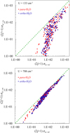Fig. 1 Comparison of H2O + H2O collision cross sections (the units are Å2) for the excitation and quenching directions of 441 state-to-state transitions at two values of collision energy U. The departure of data-points from the diagonal line (dashed) signifies the deviation from the principle of microscopic reversibility.

3 Results and discussion

In the following, we use Method 3 to compute temperature-dependent rate coefficients for excitation and quenching. From the previous work (Mandal & Babikov 2023), the values of cross sections are available at six collision energies: U = 133, 200, 267, 400, 533, and 708 cm⁻¹. These are used to compute six values of the integrand function F(U, T) at each temperature. The overall range of integration in Eqs. (18) and (19) is split onto three intervals, each treated differently: $$\begin{array}{l}{U}_0<U<200{\text{cm}}^{-1},\hfill \\ 200\le U\le 533{\text{cm}}^{-1},\hfill \\ 533<U<+\infty .\hfill \end{array}$$

Here, U₀ = ∆E/4 is a threshold where F(U, T) = 0. The values of the threshold are different for different transitions n ↔ n′ and in the database they range from U₀ = 0.05 cm⁻¹ for transition 5₂₃ ↔ 6₁₆ to U₀ = 166 cm⁻¹ for transition 6₃₃ ↔ 0₀₀ In the low-energy part of the range (from the threshold up to the second datapoint), the integral is computed analytically by constructing a three-point analytic interpolation of the first three datapoints using the following function: $$F_0\left(U\right)={\left(\frac{U-U_0}{C}\right)}^A{\text{e}}^{-\frac{U-U_0}{B}}.$$(20)

Expressions for the fitting coefficients A, B, and С are given in Appendix B. In the middle part of the range, the integration is carried out numerically by constructing a cubic spline of the datapoints and using a constant-step quadrature with a large number of points. In the high-energy interval (from the fifth datapoint to infinity), the integral is also computed analytically by constructing the analytic fit of the last three datapoints using the following function: $$F_{\infty }\left(U\right)=a{\text{e}}^{-\frac{U}{b}-{\left(\frac{U}{c}\right)}^2},$$(21)

and using this function to extrapolate to the range of large values of U. Expressions for the fitting coefficients a, b, and с are also given in Appendix B.

From Eqs. (17)–(19), it follows that having cross sections σ_n→n′·(U) for quenching and σ_n′→n(U) for excitation at our disposal, we can in principle calculate two sets of rate coefficients. Namely, using the first line of Eq. (17) to compute F(U) from σ_n→n′·(U), and then using Eqs. (18)–(19) to compute k_n→n′·(T) and k_n→n′(T), one can obtain the full set of rate coefficients for quenching and excitation from quenching cross sections alone. Alternatively, using the second line of Eq. (17) to compute F(U) from σ_n′→n(U), and then using Eqs. (18)–(19) to compute k_n→n′(T) and k_n′→n(T), one can obtain another full set of rate coefficients for quenching and excitation from excitation cross sections alone. If the microscopic reversibility is satisfied, the two sets of data should be identical.

We carried out these calculations and compared two nascent sets of rate coefficients in Fig. 2 for T = 300 K. One can see that the rate coefficients obtained from the excitation and quenching cross sections are similar overall but are not exactly the same, which means that the principle of microscopic reversibility is not exactly satisfied.

In general, there is no strong argument in favor of one of these two sets of rate coefficients. However, we note that rate coefficients for excitation and quenching form similar patterns on two sides of the diagonal line in Fig. 2, which suggests that the desired (actual) rate coefficients must be somewhere between the two sets. Therefore, it makes sense to use both excitation and quenching cross sections at the same time to produce one set of rate coefficients. This can be done by constructing, for each transition n ↔ n’′ at each temperature, the integrand function $\tilde{F}$(U, T), which represents an average of the first and second lines of Eq. (17), namely: $$\begin{array}{l}\tilde{F}\left(U,T\right)=\frac{\left(2j+1\right){\sigma }_{n\to n^{\prime }}\left(U\right)+\left(2j^{\prime }+1\right){\sigma }_{n^{\prime }\to n}\left(U\right)}{2}\hfill \\ \times U\left[1-{\left(\frac{\text{Δ}E}{4U}\right)}^2\right]{\text{e}}^{-\frac{U}{k_{\text{B}}T}\left[1+{\left(\frac{\text{Δ}E}{4U}\right)}^2\right]}.\hfill \end{array}$$(22)

We note that this formula includes both quenching and excitation cross sections σ_n→n′·(U) and σ_n′→n(U) taken as a weighted sum to generate one single integrand function. The microscopic reversibility is automatically satisfied by Eqs. (18) and (19). Figure 3 gives examples of the integrand functions $\tilde{F}$(U) constructed for three different values of temperature for all 441 transitions (ortho and para combined) in a broad energy range (from thresholds U₀ to U ~ 10⁴ cm⁻¹). One can see that these functions grow quickly at the threshold, pass through the computed datapoints smoothly, and then decay exponentially at high energy. This behavior is typical for many other molecule + atom and molecule + molecule systems.

Figures 4 and 5 report the temperature dependencies of rate coefficients for individual transitions in H₂O + H₂O obtained by integrating $\tilde{F}$(U) as explained in Appendix B, and then using Eqs. (18) and (19) to ensure microscopic reversibility. Two frames of Fig. 4 report excitation and quenching rate coefficients for 231 transitions between para-states of water, while two frames of Fig. 5 report 210 transitions between the ortho-states of water, all in the range from 10 K to 1000 K. One can see that temperature dependencies of excitation cross sections are stronger, with many transitions characterized by cross sections that decrease exponentially when the temperature is reduced. In contrast, the rate coefficients for quenching usually increase at low temperature and vary less through the covered range.

Figures 6 and 7 present a comparison of the rate coefficients computed here with our previous work (Mandal & Babikov 2023) and also with those from the work of other authors (Boursier et al. 2020; Buffa et al. 2000). As here we reuse MQCT cross sections from our previous work, the differences between our new and old results are not expected to be large. Indeed, in Figs. 6 and 7, we see that red dots do not deviate significantly from the diagonal line. Still, we see that the deviations become more noticeable at high temperatures. For example, in para-H₂O at T = 200 K, an RMS deviation of our new rate coefficients from the old ones is ~ 12% for stronger dipole-driven transitions and is ~18% for weaker transitions. At T = 800 K, these differences increase to ~30% for stronger and ~32% for weaker transitions. In ortho-H₂O at T = 200 K, the RMS difference is ~ 11 % for stronger transitions and is ~ 16% for weaker transitions. At T = 800 K, they increase to ~28% and ~29%, respectively. Therefore, our new approach, which includes integration over the range of collision energies, is preferred over the older simplified approach (where the energy dependence was neglected) and is recommended, in particular for higher temperatures.

In our previous paper, we explained in detail that, for the stronger dipole-driven transitions, our MQCT cross sections are somewhat smaller than those obtained by semi-classical methods of either Buffa et al. (2000) or Boursier et al. (2020), while for the weaker transitions our MQCT cross sections are somewhat larger than those of Boursier et al. (2020). This is also true for a set of new rate coefficients obtained here. Indeed, in the range of the larger rate coefficients of Figs. 6 and 7 (over 2 × 10⁻¹⁰ cm³ s⁻¹), blue and cyan symbols concentrate above the diagonal line, while in the range of smaller rate coefficients (under 2 × 10⁻¹⁰ cm³ s⁻¹) blue symbols are found below the diagonal line. Moreover, our new rate coefficients are somewhat smaller than our old rate coefficients, as characterized by the RMS deviations quoted in the previous paragraph. Therefore, the difference between our results and those of either Buffa et al. (2000) or Boursier et al. (2020) is slightly greater here than the differences described in our previous work Mandal & Babikov (2023), and this is accentuated at higher temperatures. These differences come from two sources, one of which is the description of molecule–molecule interactions, and another is the treatment of collision dynamics. Our MQCT calculations are expected to be better in both respects, because here we employ an accurate potential energy surface (with controlled truncation) and treat all state-to-state transitions in a self-consistent manner (including the interference of various energy-transfer pathways).

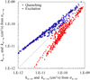Fig. 2 Comparison of two sets of rate coefficients obtained from quenching and excitation cross sections, as explained in the text. The departure of the datapoints from the diagonal line signifies deviation from the principle of microscopic reversibility. Red and blue correspond to quenching and excitation rate coefficients, respectively.

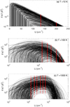Fig. 3 Energy dependence of average integrand functions $\tilde{F}$(U) from Eq. (22) for all state-to-state transitions in the H2O + H2O database, at three values of temperature. Red symbols indicate MQCT datapoints at six values of collision energy U. Solid lines are used for analytic fits and numeric splines through the temperature range.

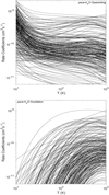Fig. 4 Temperature dependence of rate coefficients for 231 individual state-to-state transitions in the “target” para- H2O molecule. For the “collider” H2O molecule, a thermal distribution of both para- and ortho-states is assumed.

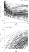Fig. 5 Temperature dependence of rate coefficients for 210 individual state-to-state transitions in a “target” ortho- H2O molecule. For the “collider” H2O molecule, a thermal distribution of both para- and ortho-states is assumed.

4 Conclusions

In this paper, we describe a new procedure for computing rate coefficients for collision-induced transitions between the rotational states of molecules in a situation when the state-to-state transition cross sections are computed using an approximate method that does not satisfy the principle of microscopic reversibility automatically. This approach is based on the method of Billing (Billing 2003), where an effective collision energy U is introduced for the calculation of both excitation and quenching directions of the same transition (instead of dealing with two different collision energies for the excitation and quenching processes). The final formulae of the symmetrized approach proposed here, Eqs. (17)–(19), are new to the best of our knowledge. They allow the use of a weighted average of excitation and quenching cross sections for the prediction of rate coefficients that satisfy the principle of microscopic reversibility. In addition, they help to interpolate cross sections between the computed datapoints and the process threshold, allowing expansion of the prediction of rate coefficients into the low-temperature regime.

We applied this method to revise the existing database of rate coefficients for the rotational state-to-state transitions in H₂O + H₂O collisions. In the older databases for H₂O + H₂O, integration over collision energy was not carried out at all. Instead, the rate coefficient was predicted approximately using one value of cross section (at the collision energy that corresponds to the average collision speed at a given temperature). Here, the actual integration over collision energy was carried out from the process threshold to infinity using extrapolation of computed cross sections into the high-energy regime. As a result, the range of temperatures was expanded from 150 ≤ T ≤ 800 K in the older database to T ≤ 1000 K in the revised database. The data presented in this paper are plotted for the temperatures above 10 K, but we also looked at the predictions of rate coefficients down to T ~ 5K, and these seem to be reasonable and follow the same trend. These data can be used for the modeling of cometary comas and planetary atmospheres where H₂O + H₂O collisions are important. For the potential users of this database, we created a computer code that generates rate coefficients for 231 transitions between the para-states of water and 210 transitions between the ortho-states of water (in both excitation and quenching directions) at any given temperature in the range 5 ≤ T ≤ 1000 K. This code is available at the CDF via anonymous ftp. The data have also been submitted to the BASEC0L database.

We note that the low-temperature predictions are based on the asymptotic form of cross-section behavior near threshold that contains no information about low-temperature quantum phenomena, such as scattering resonances, which may be important for H₂O + H₂O. For these to be described accurately, one would have to carry out the full-quantum calculations of inelastic scattering, which is computationally unaffordable. The data available for the H₂O + H₂O system at this time come either from a semi-classical method (Boursier et al. 2020; Buffa et al. 2000), or from the mixed quantum-classical theory (Mandal & Babikov 2023), which are both approximate.

It should also be noted that all databases of rate coefficients for the H₂O + H₂O system developed so far involve averaging over rotational states of “collider” H₂O molecules, assuming the Boltzman distribution at a given temperature. This is partly due to tradition, and partly due to the fact that the number of states in water is very large. For example, the present database reports 882 transitions in the “target” molecule if both excitation and quenching processes of para- and ortho-water are combined. If one chooses not to average over the states of “collider” molecules, then each transition in the “target” needs to be combined with each transition in the “collider”, leading to over 750 000 individual transitions in the H₂O + H₂O system. Even if such cross-section data are available, the energy dependence of cross sections for each transition must be fitted and integrated in an automatic but controllable manner in order to avoid mistakes. Furthermore, these must somehow be reported. The traditional way of reporting rate coefficients, namely as an ASCII file, may no longer be appropriate. Therefore, in the future, we would like to offer a database of the individual state-to-state transitions in the H₂O + H₂O system resolved in the initial and final states of both collision partners, and available as a convenient subroutine that generates rate coefficients. This would provide indispensable input data - not available at the present time – for radiation transfer modeling in H₂O-rich environments in conditions that are far from local thermodynamic equilibrium, which is rather typical in astrophysics.

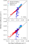Fig. 6 Comparison of rate coefficients computed here vs those available from the literature for the quenching of para-H2O states by collisions with a thermal ensemble of H2O molecules at two values of temperature.

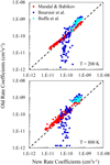Fig. 7 Comparison of rate coefficients computed here vs those available from the literature for the quenching of ortho-H2O states by collisions with a thermal ensemble of H2O molecules at two values of temperature.

Acknowledgements

This research was supported by NASA Astrophysics Research and Analysis Program. DB acknowledges the support of Way Klingler Research Fellowship and of the Pfletschinger-Habermann Research Fund. We used resources of the National Energy Research Scientific Computing Center, which is supported by the Office of Science of the U.S. Department of Energy under Contract No. DE-AC02-5CH11231. This research also used HPC resources at Marquette funded in part by the National Science foundation award CNS-1828649. Marie-Lise Dubernet at the Observatory of Paris is gratefully acknowledged for her continuous support of these efforts. Martin Cordiner at NASA is acknowledged for stimulating discussions and his encouragement of this project.

Appendix A The unitless approach

Let us introduce a unitless variable, u = 4U/∆E, for each transition independently. In a sense, и measures the value of U in the units of its minimal value, ∆E/4. Further, the range of this unitless variable is always the same, и > 1. Also, let us introduce another unitless variable that measures k_BT in the units of ∆E/4, namely: ε = 4k_BT/∆E. Using these definitions, Eqs. (17)–(19) of Method 3 can be rewritten as follows: $$\begin{array}{l}F\left(u,\epsilon \right)=\left(2j+1\right){\sigma }_{n\to n^{\prime }}\left(u\right)\left[u-\frac{1}{u}\right]{\text{e}}^{-\left[u+\frac{1}{u}\right]/\epsilon }\hfill \\ =\left(2j^{\prime }+1\right){\sigma }_{n^{\prime }\to n}\left(u\right)\left[u-\frac{1}{u}\right]{\text{e}}^{-\left[u+\frac{1}{u}\right]/\epsilon }\hfill \end{array}$$

and for the rate coefficients: $$k_{n\to n^{\prime }}\left(T\right)=\frac{{\upsilon }_{\text{ave}}\left(T\right)}{{\epsilon }^2}\left(\frac{{\text{e}}^{+2/\epsilon }}{2j+1}\right){\displaystyle \underset{u=1}{\overset{\infty }{\int }}F\left(u,\epsilon \right)du},$$ $$k_{n^{\prime }\to n}\left(T\right)=\frac{{\upsilon }_{\text{ave}}\left(T\right)}{{\epsilon }^2}\left(\frac{{\text{e}}^{-2/\epsilon }}{2j^{\prime }+1}\right){\displaystyle \underset{u=1}{\overset{\infty }{\int }}F\left(u,\epsilon \right)du}.$$

In these expressions, all variables are unitless, except cross sections and collision velocities. Importantly, the integration range is independent of ∆E. It is easy to see that in the high-energy limit, и → ∞, the expression for integrand simplifies and is similar in appearance to that of Eqs. (1) and (3), e.g.: $$\begin{array}{l}F\left(u,\epsilon \right)\sim \left(2j+1\right)u{\sigma }_{n\to n^{\prime }}\left(u\right){\text{e}}^{-u/\epsilon }\hfill \\ \sim \left(2j+1\right)u{\sigma }_{n\to n^{\prime }}\left(u\right){\text{e}}^{-u/\epsilon }.\hfill \end{array}$$

This unitless formulation of Method 3 may be advantageous for some applications.

Appendix B The fitting formulae

B.1 Low-energy range

Using three data points with the values of energy U₁, U₂, and U₃ and the corresponding values of the function F₁, F₂, and F₃ on the low-energy side, the fitting coefficients for Eq. (20) are obtained as follows: $$A=\frac{\left(U_3-U_1\right)ln\left(F_2/F_1\right)-\left(U_2-U_1\right)ln\left(F_3/F_1\right)}{\left(U_3-U_1\right)ln\left(U_2/U_1\right)-\left(U_2-U_1\right)ln\left(U_3/U_1\right)},$$

then $$B=\frac{\left(U_2-U_1\right)}{ln\left[\left(\frac{F_1}{F_2}\right){\left(\frac{U_2-U_0}{U_1-U_0}\right)}^A\right]},$$

and then $$C=\frac{\left(U_1-U_0\right)}{F_1^{1/A}}exp\left(-\frac{U_1-U_0}{AB}\right).$$

Unfortunately, analytic integration of $\tilde{F}$(U) in the form of Eq. (20) requires calculations of the incomplete gamma-function γ(A + 1, U₂/B); see Gradshteyn & Ryzhik (Table of Integrals, Series and Products). To avoid this complication, we set A = 1, which is equivalent to using a two-point fitting formula. Then, using coefficients B and C only, the integral of $\tilde{F}$(U) in the range from U₀ to U₂ is computed easily: $$\begin{array}{l}{\displaystyle \underset{U_0}{\overset{U_2}{\int }}{\tilde{F}}_0\left(U\right)dU={\displaystyle \underset{U_0}{\overset{U_2}{\int }}\left(\frac{U-U_0}{C}\right){\text{e}}^{-\frac{U-U_0}{B}}dU}}\hfill \\ =\frac{B^2}{C}\left[1-\left(\frac{C}{U_2-U_0}+\frac{C}{B}\right)F_2\right].\hfill \end{array}$$

B.2 High-energy range

Similar, using three data points with the values of energy U4, U₅, and U₆ and the corresponding values of the function F₄, F₅, and F₆ at the high-energy side, the coefficients for Eq. (24) are obtained as follows: $$\begin{array}{l}b=\frac{\left(U_5-U_4\right)\left(U_6-U_5\right)\left(U_6-U_6\right)}{\left(U_6^2-U_4^2\right)ln\left(F_6/F_5\right)-\left(U_6^2-U_5^2\right)ln\left(F_6/F_4\right)},\hfill \\ c=\sqrt{\frac{\left(U_5-U_4\right)\left(U_6-U_5\right)\left(U_6-U_6\right)}{\left(U_6-U_5\right)ln\left(F_6/F_4\right)-\left(U_6-U_4\right)ln\left(F_6/F_5\right)},}\hfill \end{array}$$

then $$a=F_6{\text{e}}^{\frac{U_6}{b}+{\left(\frac{U_6}{c}\right)}^2}.$$

It is assumed that c² ≥ 0. At high temperatures (near T =800 K), for some transitions the last data point (at U₆ =708 cm⁻¹) seems to be inaccurate (most likely due to thermal averaging over the states of quencher), which causes c² to be negative. In such cases, we disregard this last point and simply use the previous one. If c² is still negative (very rare), we set c = +∞ and use a two-point fitting formula.

Using coefficients a, b, and c, the integral of $\tilde{F}$(U) in the range from U₅ to +∞ is computed analytically: $$\begin{array}{l}{\displaystyle \underset{U_5}{\overset{\infty }{\int }}{\tilde{F}}_{\infty }\left(U\right)dU={\displaystyle \underset{U_5}{\overset{\infty }{\int }}a{\text{e}}^{-\frac{U}{b}-{\left(\frac{U}{c}\right)}^2}dU}}\hfill \\ =\frac{\sqrt{\pi }}{2}ac\times exp\left(\frac{c^2}{4b^2}\right)\left[1-\text{erf}\left(\frac{2b{U}_5+c^2}{2bc}\right)\right].\hfill \end{array}$$

The last two factors in this formula can become very large and very small simultaneously, which causes practical difficulty for some transitions. A convenient way to deal with such an error function is to use an approximate expression: $$\text{erf}\left(x\right)=1-P\left\{x\right\}{\text{e}}^{-x^2},$$

where P{x} is a fifth-order polynomial of the form given by Abramovitz & Stegun (Handbook of Mathematical Functions with Formulas, Graphs and Mathematical Tables). This permits expression of the integral through the value of F₅ and the polynomial, as follows: $${\displaystyle \underset{U_5}{\overset{\infty }{\int }}{\tilde{F}}_{\infty }\left(U\right)dU=\frac{\sqrt{\pi }}{2}c{F}_{5}P}\left\{\frac{2b{U}_5+c^2}{2bc}\right\}.$$

When the two-point extrapolation is used, the expression is: $${\displaystyle \underset{U_5}{\overset{\infty }{\int }}{\tilde{F}}_{\infty }\left(U\right)dU={\displaystyle \underset{U_5}{\overset{\infty }{\int }}a{\text{e}}^{-\frac{U}{b}}dU=b{F}_5}.}$$

References

All Figures

	Fig. 1 Comparison of H2O + H2O collision cross sections (the units are Å2) for the excitation and quenching directions of 441 state-to-state transitions at two values of collision energy U. The departure of data-points from the diagonal line (dashed) signifies the deviation from the principle of microscopic reversibility.
In the text

	Fig. 2 Comparison of two sets of rate coefficients obtained from quenching and excitation cross sections, as explained in the text. The departure of the datapoints from the diagonal line signifies deviation from the principle of microscopic reversibility. Red and blue correspond to quenching and excitation rate coefficients, respectively.
In the text

	Fig. 3 Energy dependence of average integrand functions $\tilde{F}$(U) from Eq. (22) for all state-to-state transitions in the H2O + H2O database, at three values of temperature. Red symbols indicate MQCT datapoints at six values of collision energy U. Solid lines are used for analytic fits and numeric splines through the temperature range.
In the text

	Fig. 4 Temperature dependence of rate coefficients for 231 individual state-to-state transitions in the “target” para- H2O molecule. For the “collider” H2O molecule, a thermal distribution of both para- and ortho-states is assumed.
In the text

	Fig. 5 Temperature dependence of rate coefficients for 210 individual state-to-state transitions in a “target” ortho- H2O molecule. For the “collider” H2O molecule, a thermal distribution of both para- and ortho-states is assumed.
In the text

	Fig. 6 Comparison of rate coefficients computed here vs those available from the literature for the quenching of para-H2O states by collisions with a thermal ensemble of H2O molecules at two values of temperature.
In the text

	Fig. 7 Comparison of rate coefficients computed here vs those available from the literature for the quenching of ortho-H2O states by collisions with a thermal ensemble of H2O molecules at two values of temperature.
In the text

References

- Al-Edhari, A. J., Ceccarelli, C, Kahane, C, et al. 2017, A & A, 597, A40 [NASA ADS] [CrossRef] [EDP Sciences] [Google Scholar]
- Billing, G. D. 1984, Comput. Phys. Rep. (Netherlands), 1 [Google Scholar]
- Billing, G. D. 2003, The Quantum Classical Theory (Oxford University Press) [CrossRef] [Google Scholar]
- Bockelée-Morvan, D., Hartogh, P., Crovisier, J., et al. 2010, A & A, 518, A149 [Google Scholar]
- Bonev, B. P., Russo, N. D., DiSanti, M. A., et al. 2021, Planet. Sei. J., 2, 45 [CrossRef] [Google Scholar]
- Bostan, D., Mandal, В., Joy, C, & Babikov, D. 2023, Phys. Chem. Chem. Phys., 25, 15683 [NASA ADS] [CrossRef] [Google Scholar]
- Boursier, С, Mandal, В., Babikov, D., & Dubernet, M. 2020, MNRAS, 498, 5489 [NASA ADS] [CrossRef] [Google Scholar]
- Bruzzone, L., Plaut, J. J., Alberti, G., et al. 2013, in 2013 IEEE International Geoscience and Remote Sensing Symposium-IGARSS, IEEE, 3907 [CrossRef] [Google Scholar]
- Buffa, G., Tarrini, O., Scappini, E, & Cecchi-Pestellini, C. 2000, ApJS, 128, 597 [NASA ADS] [CrossRef] [Google Scholar]
- Cochran, A. L., Levasseur-Regourd, A.-C., Cordiner, M., et al. 2015, Space Sei. Rev, 197, 9 [NASA ADS] [CrossRef] [Google Scholar]
- Cordiner, M., Milam, S., Biver, N., et al. 2020, Nat. Astron., 4, 861 [NASA ADS] [CrossRef] [Google Scholar]
- Cordiner, M., Coulson, I., Garcia-Berrios, E., et al. 2022, ApJ, 929, 38 [CrossRef] [Google Scholar]
- Daniel, F., Dubernet, M.-L., & Grosjean, A. 2011, A & A, 536, A76 [CrossRef] [EDP Sciences] [Google Scholar]
- Dones, L., Brasser, R., Kaib, N., & Rickman, H. 2015, Space Sei. Rev, 197, 191 [NASA ADS] [CrossRef] [Google Scholar]
- Dubernet, M.-L., & Quintas-Sánchez, E. 2019, Mol. Astrophys., 16, 100046 [NASA ADS] [CrossRef] [Google Scholar]
- Enya, K., Kobayashi, M., Kimura, J., et al. 2022, Adv. space Res., 69, 2283 [NASA ADS] [CrossRef] [Google Scholar]
- Faure, A., & Josselin, E. 2008, A & A, 492, 257 [CrossRef] [EDP Sciences] [Google Scholar]
- Faure, A., Wiesenfeld, L., Wernli, M., & Valiron, P. 2005, J. Chem. Phys., 123, 104309 [NASA ADS] [CrossRef] [Google Scholar]
- Faure, A., Lique, F., & Remijan, A. J. 2018, J. Phys. Chem. Lett., 9, 3199 [NASA ADS] [CrossRef] [Google Scholar]
- Faure, A., Lique, F., & Loreau, J. 2020, MNRAS, 493, 776 [NASA ADS] [CrossRef] [Google Scholar]
- Green, S., & Thaddeus, P. 1976, ApJ, 205, 766 [NASA ADS] [CrossRef] [Google Scholar]
- Hartogh, P., Lis, D.C., Bockelée-Morvan, D., et al. 2011, Nature, 478, 218 [NASA ADS] [CrossRef] [Google Scholar]
- Joy, C., Mandal, В., Bostan, D., & Babikov, D. 2023, Phys. Chem. Chem. Phys., 25, 17287 [NASA ADS] [CrossRef] [Google Scholar]
- Khalifa, M. В., Quintas-Sánchez, E., Dawes, R., Hammami, К., & Wiesenfeld, L. 2020, Phys. Chem. Chem. Phys., 22, 17494 [NASA ADS] [CrossRef] [Google Scholar]
- Levine, R. D. 2011, Quantum Mechanics of Molecular Rate Processes (Courier Corporation) [Google Scholar]
- Loreau, J., Faure, A., & Lique, F. 2018, J. Chem. Phys., 148, 244308 [NASA ADS] [CrossRef] [Google Scholar]
- Mandal, В., & Babikov, D. 2023, A & A, 671, A51 [NASA ADS] [CrossRef] [EDP Sciences] [Google Scholar]
- Mandal, В., Semenov, A., & Babikov, D. 2018, J. Phys. Chem. A, 122, 6157 [NASA ADS] [CrossRef] [Google Scholar]
- Mandal, В., Semenov, A., & Babikov, D. 2020, J. Phys. Chem. A, 124, 9877 [NASA ADS] [CrossRef] [Google Scholar]
- Mandal, В., Joy, С., Semenov, А., & Babikov, D. 2022, ACS Earth Space Chem., 6, 521 [NASA ADS] [CrossRef] [Google Scholar]
- Roth, N. X., Bonev, B. P., DiSanti, M. A., et al. 2021, Planet. Sei. J., 2, 54 [CrossRef] [Google Scholar]
- Semenov, A., & Babikov, D. 2014a, J. Phys. Chem. Lett., 5, 275 [CrossRef] [Google Scholar]
- Semenov, A., & Babikov, D. 2014b, J. Chem. Phys., 140, 044306 [NASA ADS] [CrossRef] [Google Scholar]
- Semenov, A., & Babikov, D. 2015, J. Phys. Chem. Lett., 6, 1854 [CrossRef] [Google Scholar]
- Semenov, A., & Babikov, D. 2016, J. Phys. Chem. A, 120, 3861 [NASA ADS] [CrossRef] [Google Scholar]
- Semenov, A., Ivanov, M., & Babikov, D. 2013, J. Chem. Phys., 139, 074306 [NASA ADS] [CrossRef] [Google Scholar]
- Semenov, A., Mandal, В., & Babikov, D. 2020, Comput. Phys. Commun., 252, 107155 [NASA ADS] [CrossRef] [Google Scholar]
- Sun, Z.-F., van Hemert, M.C., Loreau, J., et al. 2020, Science, 369, 307 [NASA ADS] [CrossRef] [Google Scholar]
- Vorburger, A., Fatemi, S., Galli, A., et al. 2022, Icarus, 375, 114810 [NASA ADS] [CrossRef] [Google Scholar]
- Wiesenfeld, L. 2021, J. Chem. Phys., 155, 071104 [NASA ADS] [CrossRef] [Google Scholar]
- Wiesenfeld, L., & Faure, A. 2010, Phys. Rev. A, 82, 040702 [NASA ADS] [CrossRef] [Google Scholar]
- Wiesenfeld, L., Scribano, Y., & Faure, A. 2011, Phys. Chem. Chem. Phys., 13, 8230 [NASA ADS] [CrossRef] [Google Scholar]
- Wirström, E., Bjerkeli, P., Rezac, L., Brinch, C., & Hartogh, P. 2020, A & A, 637, A90 [CrossRef] [EDP Sciences] [Google Scholar]
- Żółtowski, M., Loreau, J., & Lique, F. 2022, Phys. Chem. Chem. Phys., 24, 11910 [CrossRef] [Google Scholar]