| Issue |
A&A
Volume 674, June 2023
|
|
|---|---|---|
| Article Number | A90 | |
| Number of page(s) | 12 | |
| Section | Planets and planetary systems | |
| DOI | https://doi.org/10.1051/0004-6361/202346298 | |
| Published online | 07 June 2023 | |
KMT-2021-BLG-2010Lb, KMT-2022-BLG-0371Lb, and KMT-2022-BLG-1013Lb: Three microlensing planets detected via partially covered signals
1
Department of Physics, Chungbuk National University,
1 Chungdae-ro, Seowon-gu,
Cheongju, Republic of Korea
e-mail: cheongho@astroph.chungbuk.ac.kr
2
Korea Astronomy and Space Science Institute,
776 Daedeok-daero, Yuseong-gu,
Daejon
34055, Republic of Korea
3
Center for Astrophysics,
Harvard & Smithsonian 60 Garden St.,
Cambridge, MA
02138, USA
4
Department of Astronomy and Tsinghua Centre for Astrophysics, Tsinghua University,
Beijing
100084, PR China
5
Auckland Observatory,
670 Manukau Road, Epsom,
Auckland
1345, New Zealand
6
University of Canterbury, Department of Physics and Astronomy,
Private Bag 4800,
Christchurch
8020, New Zealand
7
Max Planck Institute for Astronomy,
Königstuhl 17,
69117
Heidelberg, Germany
8
Department of Astronomy, The Ohio State University,
140 W. 18th Ave.,
Columbus, OH
43210, USA
9
Department of Particle Physics and Astrophysics,
Weizmann Institute 56,
Rehovot
76100, Israel
10
School of Space Research, Kyung Hee University,
Yongin, Kyeonggi
17104, Republic of Korea
11
Korea University of Science and Technology,
217 Gajeong-ro, Yuseong-gu,
Daejeon,
34113, Republic of Korea
12
Institute for Radio Astronomy and Space Research (IRASR), AUT University,
55 Wellesley Street East, Auckland CBD,
Auckland
1010, New Zealand
13
National Astronomical Observatories, Chinese Academy of Sciences,
Beijing
100101, PR China
14
School of Physics and Astronomy, Tel-Aviv University,
Tel-Aviv
6997801, Israel
15
Department of Physics and Astronomy, Louisiana State University,
202 Nicholson Hall,
Baton Rouge, LA
70803, USA
Received:
2
March
2023
Accepted:
7
April
2023
Aims. We inspect the four microlensing events KMT-2021-BLG-1968, KMT-2021-BLG-2010, KMT-2022-BLG-0371, and KMT-2022-BLG-1013, for which the light curves exhibit partially covered short-term central anomalies. We conduct detailed analyses of the events with the aim of revealing the nature of the anomalies.
Methods. We tested various models that can explain the anomalies of the individual events, including the binary-lens (2L1S) and binary-source (1L2S) interpretations. Under the 2L1S interpretation, we thoroughly inspected the parameter space to determine the existence of degenerate solutions, and if they existed, we tested whether the degeneracy could be resolved.
Results. We find that the anomalies in KMT-2021-BLG-2010 and KMT-2022-BLG-1013 are uniquely defined by planetary-lens interpretations with planet-to-host mass ratios of q ~ 2.8 × 10⁻³ and ~1.6 × 10⁻³, respectively. For KMT-2022-BLG-0371, a planetary solution with a mass ratio q ~ 4 × 10⁻⁴ is strongly favored over the other three degenerate 2L1S solutions with different mass ratios based on the χ2 and relative proper motion arguments, and a 1L2S solution is clearly ruled out. For KMT-2021-BLG-1968, on the other hand, we find that the anomaly can be explained either by a planetary or a binary-source interpretation, making it difficult to firmly identify the nature of the anomaly. From the Bayesian analyses of the identified planetary events, we estimate that the masses of the planet and host are (Mp/MJ, Mh/M⊙) = (1.07−0.68+1.15, 0.37−0.23+0.40), (0.26−0.11+0.13, 0.63−0.28+0.32), and (0.31−0.16+0.46, 0.18−0.10+0.28) for KMT-2021-BLG-2010L, KMT-2022-BLG-0371L, and KMT-2022-BLG-1013L, respectively.
Key words: gravitational lensing: micro / planets and satellites: detection
© The Authors 2023
 Open Access article, published by EDP Sciences, under the terms of the Creative Commons Attribution License (https://creativecommons.org/licenses/by/4.0), which permits unrestricted use, distribution, and reproduction in any medium, provided the original work is properly cited.
This article is published in open access under the Subscribe to Open model. Subscribe to A&A to support open access publication.
1 Introduction
Current planetary microlensing experiments are being carried out with the use of multiple wide-field telescopes. With the high observational cadence achieved by employing large-format cameras and continuous coverage using multiple telescopes, the experiments aim to construct a large planet sample that includes terrestrial planets. The microlensing planet sample is of scientific importance in studying the demographic distribution of planets because it includes planet populations for which the detection efficiency of other major planet detection methods is low, for example, cold planets with faint host stars.
Despite the enhanced observational cadence of the current microlensing surveys, the coverage for a fraction of planet-induced signals can be incomplete, especially for signals with short durations. The most common cause for the incomplete coverage is bad weather. The three telescopes of the Korea Microlensing Telescope Network (KMTNet; Kim et al. 2016) experiment are located in the three continents of the Southern Hemisphere. They include the Siding Spring Observatory in Australia (KMTA), the Cerro Tololo Interamerican Observatory in Chile (KMTC), and the South African Astronomical Observatory in South Africa (KMTS). When one of these telescope sites is clouded out, the coverage of a signal with a duration shorter than about one day produced by a low-mass planet would be incomplete. Another cause for the incomplete anomaly coverage is that the subset of survey fields is observed with a relatively low cadence. The observational cadence for the peripheral fields of the KMTNet survey is 4–20 times lower than the 0.25 hr cadence of the prime fields, and thus the coverage of a short-duration signal detected in these low-cadence fields can be incomplete. Examples are the planetary events KMT-2017-BLG-0673 and KMT-2019-BLG-0414 (Han et al. 2022a). In addition, the coverage of signals detected in the early or late phase of a bulge season can also be incomplete: In the two-planet event OGLE-2019-BLG-0468 (Han et al. 2022b), the target rises and sets close to twilight.
We present the analyses of the four microlensing events KMT-2021-BLG-1968, KMT-2021-BLG-2010, KMT-2022-BLG-0371, and KMT-2022-BLG-1013, for which the light curves of the events exhibit partially covered short-term central anomalies. With the aim of revealing the nature of the anomalies, we conduct detailed analyses of the events under various interpretations that can explain the anomalies of the individual events.
We present the analyses of the events according to the following organization. In Sect. 2, we describe the acquisition and reduction procedure of the data used in the analyses. In Sect. 3, we depict the models we tested for the interpretations of the anomalies, and introduce parameters used in the modeling. In the subsequent subsections, we present the detailed analyses we conducted for the events KMT-2021-BLG-1968 (Sect. 3.1), KMT-2021-BLG-2010 (Sect. 3.2), KMT-2022-BLG-0371 (Sect. 3.3), and KMT-2022-BLG-1013 (Sect. 3.4). Based on these analyses, we judge whether the anomalies have a planetary origin. In Sect. 4, we specify the source stars of the events by estimating the colors and magnitudes, and we estimate the angular Einstein radii. In Sect. 5, we estimate the physical parameters of the mass and distance to the identified planetary systems. We summarize our results in Sect. 6.
2 Observations and data
All the lensing events analyzed this work were detected in the 2021 and 2022 seasons by the KMTNet survey from the monitoring of stars lying toward the Galactic bulge field. The three telescopes used by the KMTNet survey are identical, and each 1.6 m telescope is equipped with a camera yielding a field of view of 4 deg2. Since July 2020, the MAP & µFUN Follow-up teams have been conducting a long-term follow-up program for high-magnification events (Zang et al. 2021). For the two very high magnification events KMT-2022-BLG-0371 and KMT-2022-BLG-1013, observations were additionally conducted using the 1 m telescopes of the Las Cumbres Observatory global network at CTIO (LCOC) and SAAO (LCOS) for KMT-2022-BLG-0371 and KMT-2022-BLG-1013, and using the 0.4 m telescope at the Auckland Observatory in New Zealand for KMT-2022-BLG-1013. KMTNet also went into follow-up mode and increased its observational cadence over the peaks of these two high-magnification events. Images from the KMTNet survey and MAP follow-up observations were mostly acquired in the I band, and a fraction of KMTNet images were obtained in the V band to measure the source color. The Auckland Observatory data were taken in the Wratten #12 filter.
Image reductions and source star photometry of the KMT-Net, LCO, and Auckland data were made with the use of the pySIS pipeline developed by Albrow et al. (2009) and Yang et al. (in prep.) on the basis of the difference-image method (Tomaney & Crotts 1996; Alard & Lupton 1998). The error bars of the data estimated by the individual photometry codes were readjusted following the routine of Yee et al. (2012) so that they are consistent with the scatter of data and the χ2 per degree of freedom (dof) for each data set becomes unity.
3 Analyses
The anomalies in the lensing light curves of the events analyzed in this work were identified from the visual inspection of the microlensing data collected during the 2021 and 2022 seasons. The common characteristic of the events and the anomalies appearing in their lensing light curves is that the peak magnifications of the events are very high, with Apeak ~ 100, 60, 570, and 280 for KMT-2021-BLG-1968, KMT-2021-BLG-2010, KMT-2022-BLG-0371, and KMT-2022-BLG-1013, respectively, and the anomalies appear near the peaks of the light curves. Three channels can produce central anomalies like this: the planetary, binary-lens, and binary-source channels.
A central anomaly through the planetary channel arises when a source star passes through the central anomaly region that forms around the tiny caustic induced by a planetary companion to the primary lens. A planetary companion induces two sets of caustics, in which one caustic (the central caustic) forms near the position of the planet host (Chung et al. 2005), and the other caustic (the planetary caustic) forms away from the host at a position ~s − 1/s (Han 2006), where s denotes the host-planet separation vector with its length scaled to the angular Einstein radius θE. Then, it is highly likely that the peak region of a high-magnification event, resulting from the close approach of the source to the planet host, is perturbed by a planet (Griest & Safizadeh 1998).
A binary lens with roughly equal-mass components can also induce a central anomaly. In the binary case, a single caustic forms near the barycenter of a close binary lens with s ≪ 1, while two caustics form near the positions of the individual lens components of a wide binary lens with s ≫ 1. Then, a central perturbation of a high-magnification event resulting from the close approach of the source either to the barycenter of the close binary or to each component of a wide binary is highly likely (Han & Hwang 2009).
A central anomaly can also arise when the closely spaced components of a binary source approach the lens successively. In this case, the resulting light curve is the superposition of the light curves of the events involved with the individual source stars, and the combined magnifications can appear to be anomalous.
We analyzed the individual lensing events by modeling the light curves under the planetary, binary-lens, and binary-source interpretations. In each modeling, we searched for a lensing solution that specified a set of lensing parameters that depict the lensing light curve. In the simplest case of a lensing event that involves a single lens and a single source (1L1S), the lensing light curve is described by three basic lensing parameters t0, u0, and tE, which denote the time of the source star’s closest approach to the lens, the lens-source separation (impact parameters) at that time, and the Einstein time scale, respectively. The impact parameter is scaled to θE, and the Einstein timescale is defined as the time it takes for the source to transit the Einstein radius. In the planetary and binary-lens cases, the lens system is composed of two lens masses and a single source (2L1S), and the inclusion of an additional lens component requires including additional parameters to depict the lens binarity. These additional parameters are s, q, and α, and the first two parameters denote the projected separation (normalized to θE) and mass ratio of the lens components, respectively, and the last parameter represents the angle between the source trajectory and the binary-lens axis (source trajectory angle). In the binary-source case, the lens system comprises a single lens and two source stars (1L2S), and the addition of the additional source requires including the three additional parameters t0,2, u0,2, and qF, which denote the approach time and impact parameter of the source companion, and the flux ratio of the two source stars, respectively (Hwang et al. 2013). In all tested models, we included an additional parameter ρ, which is defined as the ratio of the angular source radius to θE (normalized source radius), to consider finite-source effects, which may affect the lensing light curves of high-magnification events when the lens passes over the surface of a source or a central caustic. The 1L2S model contains two source stars, and we denote the normalized radius of the secondary source as ρ2. In the following subsections, we explain the detailed modeling we conducted for the individual events.
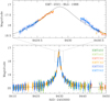 |
Fig. 1 Light curve of KMT-2021-BLG-1968. The lower panel shows the whole view, and the upper panel shows the enlarged view of the peak region around the anomaly. The 1L1S model curve is plotted over the data. |
3.1 KMT-2021-BLG-1968
The event KMT-2021-BLG-1968 occurred on a source lying at the equatorial coordinates (RA, Dec)J2000 = (17:52:25.77, −28:09:05.87), which correspond to the Galactic coordinates (l, b) = (1°.443, −0°.878). The source position corresponds to the KMTNet prime fields of BLG02 and BLG42, toward which observations were conducted with a 0.5 h cadence for each field, and a 0.25 h in combination. The extinction toward the field, A1 ~ 4.1, was high because the field lies close to the Galactic center. Together with the faintness of the source, the measurement of the source baseline was difficult, but the source was registered in the Dark Energy Camera (DECam) catalog with an i-band baseline magnitude of ibase = 21.83. The KMTNet alert of the event was issued on 2021 August 2, which corresponds to the abridged heliocentric Julian data of HJD′ ≡ HJD − 2 450 000 = 9428. The event reached its peak a day after the alert at HJD′ = 9429.8 with a peak magnitude of Ipeak ~ 17.4. The event was observed solely by the KMTNet survey without any follow-up observations.
The light curve of KMT-2021-BLG-1968 is displayed in Fig. 1, in which the lower panel shows the whole view and the upper panel shows the peak region of the light curve. The curve drawn over the data points is a point-source point-lens (PSPL) model. It shows that a short-term anomaly with a duration of about 1 day occurred near the peak of the light curve. The residual from the PSPL model presented in the bottom panel of Fig. 2 shows that negative and positive deviations occurred in the rising and falling parts, respectively. The time gap between the anomaly regions covered by the KMTC and KMTS data sets corresponds to the night time of the KMTA site, but observations at the Australian site were prevented by bad weather.
To interpret the anomaly, we first conducted a 2L1S modeling of the light curve. Figure 3 shows the ∆χ2 map obtained from the grid searches for the binary lens parameters s and q. The map shows a unique pair of local minima at (log s, log q) ~ (±0.2, −2.5) resulting from the close-wide degeneracy (Dominik 1999; An 2005). In Table 1, we list the full lensing parameters of the close (s < 1) and wide (s > 1) 2L1S solutions obtained after refining the solutions by allowing all parameters to vary. The degeneracy between the solutions is very severe with ∆χ2 < 1. For both solutions, the estimated mass ratios of the lens components, q ~ 3.1 × 10⁻³, are very low, indicating that the companion to the lens is a planet according to the 2L1S interpretation. The model curve (solid curve) of the close planetary solution is drawn over the data points in the top panel of Fig. 2, and the residuals of the close and wide solutions are presented in the lower panels. The lens-system configurations of the close and wide 2L1S solutions are presented in the left two insets of the top panel of Fig. 2. They show that the anomaly was produced by the source passage through the anomaly region extending from the protruding cusp of the central caustic induced by a planetary companion. The measured event timescale is tE ~ 20 days. The normalized source radius cannot be accurately measured due to the non-caustic-crossing nature of the anomaly, and only the upper limit ρmax ~ 4 × 10⁻³ is constrained.
We determined whether the anomaly might be explained by introducing a source companion in an additional 1L2S modeling. The lensing parameters of the best-fit 1L2S solution are listed in Table 1. The fact that qF ~ 0.12 indicates that the secondary source is fainter than the primary source, and the fact that t0 < t0,2 and u0 < u0,2 indicates that the secondary source trailed the primary source and approached closer to the lens than the primary source. The model curve (dotted curve) and the residual of the binary-source solution together with the configuration of the 1L2S lens system are presented in Fig. 1. In principle, binary source models sometimes show measurable color-dependent effects, for example, MOA-2012-BLG-486 (Hwang et al. 2013). However, because of the high extinction, the event is too faint in the V band to carry out these tests.
We find that the observed anomaly in the lensing light curve is almost equally well explained with the planetary and binary-source interpretations. From the comparison of the fits, it is found that the planetary solution is preferred over the binary-source solution by a mere ∆χ2 = 3.0. We note that resolving the degeneracy between the planetary and binary-source solutions would be difficult even if the gap between the KMTC and KMTS data sets had been covered by the KMTA data because the two models in the gap region are almost identical.
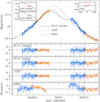 |
Fig. 2 Light curve of KMT-2021-BLG-1968 in the region of the anomaly. The curves drawn over the data points are 2L1S, 1L2S, and PSPL models, and the lower four panels show the residuals from the individual models. The three insets in the top panel show the lens-system configurations of the close and wide 2L1S solutions and the 1L2S solution. For each 2L1S configuration, the cuspy red figure represents the caustic, and the arrowed line indicates the source trajectory. For the 1L2S configuration, the small filled dot represents the lens position, and the arrowed lines marked in red and blue represent the trajectories of the primary and secondary source stars, respectively. |
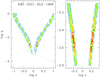 |
Fig. 3 ∆χ2 map on the (log s, log q) plane obtained from the 2L1S modeling of KMT-2021-BLG-1968. The right panel shows the enlargement of the map around the local minima. The colors represent points with ∆χ2 ≤ 1nσ (red), ≤ 2nσ (yellow), ≤ 3nσ (green), and ≤ 4nσ (cyan), where n = 3. |
Model parameters of KMT-2021-BLG-1968.
3.2 KMT-2021-BLG-2010
The lensing event KMT-2021-BLG-2010 occurred on a source lying at (RA, Dec)J2000 = (17:52:02.04, −32:16:11.10), (l, b) = (−2°.148, −2°.899), toward which the I-band extinction is AI ~ 2.1. The source lies in the KMTNet prime field of BLG41 and the sub-prime field BLG22, toward which the combined observational cadence is 0.33 h. The event was observed solely by the KMTNet group, who issued the alert of the event on 2021 August 03 (HJD′ = 9429) at around the time when the event reached its peak.
In Fig. 4, we present the light curve of KMT-2021-BLG-2010. The light curve is constructed with the use of the KMTC and KMTS data sets alone because the photometry quality of the KMTA data set is poor. It is found that the light curve exhibits an anomaly that appears around the peak with an approximate duration of one day, and the deviation from the PSPL model appears both in the rising and falling parts, as shown in the PSPL residual presented in the bottom panel of Fig. 5. Similar to the case of KMT-2021-BLG-1968, the coverage of the anomaly is incomplete due to the absence of the KMTA data set1.
We find that the anomaly of the event is uniquely explained by a pair of planetary models. In Fig. 6, we present the ∆χ2 map obtained from the grid searches for the binary parameters s and q. The estimated binary parameters are (log s, log q) ~ (± 0.06, −2.6), indicating that the anomaly was produced by a planetary companion and that the two solutions result from the close-wide degeneracy. The final lensing parameters of the close and wide planetary solutions are listed in Table 2, and the model curve of the close 2L1S solution is drawn over the data points in the top panel of Fig. 5. The residuals from both the close and wide 2L1S solutions are shown in the lower panels. We also present the lens-system configurations of the close and wide 2L1S solutions in the insets of the top panel. According to the solutions, the anomaly was produced by the source passage through the negative deviation region formed in the back-end region of the central caustic induced by a planet. The source did not cross the caustic, and thus only the upper limit of the normalized source radius, ρmax ~ 5 × 10⁻³, is constrained.
We find that the planetary and binary-source models can be distinguished with a high confidence level of ∆;χ2 = 62.7. The model curve and the residual of the best-fit 1L2S solution are presented in Fig. 5, showing that the model results in a poor fit especially in the region 9429.2 ≲ HJD′ ≲ 9429.5, which was covered by the KMTS data set.
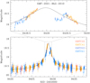 |
Fig. 4 Light curve of KMT-2021-BLG-2010. The layout and scheme of the plots are same as those of Fig. 1. |
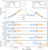 |
Fig. 5 Zoom of the central anomaly region of KMT-2021-BLG-2010. The lower four panels show the residuals from the close and wide 2L1S, 1L2S, and PSPL models. The two insets in the top panel show the lens-system configurations of the close and wide 2L1S solutions. |
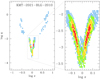 |
Fig. 6 ∆χ2 map from the 2L1S modeling of KMT-2021-BLG-2010. The notations and color scheme of the plots are same as those of Fig. 3, except that n = 2. |
3.3 KMT-2022-BLG-0371
The source of the lensing event KMT-2022-BLG-0371 lies at (RA, Dec)J2000 = (17:41:26.86, −34:41:55.21), (l, b) = (−5º.372, −2º.267). The I-band extinction toward the field is AI = 2.18. The event was found on 2022 April 11 (HJD′ = 9680), when the source became brighter than the baseline magnitude of Ibase = 19.72 by 0.45 mag. The source location corresponds to the KMTNet sub-prime field BLG37, toward which observations were carried out with a 2.5 h cadence. The event reached its peak at HJD′ = 9689.4 with a very a high magnification of Amax ~ 570. Four days before the event reached the peak (HJD′ = 9685.27), a high-magnification alert was issued by the KMTNet HighMagFinder system (Yang et al. 2022). In response to this alert, two days before the peak, follow-up observations were conducted using the LCOC and LCOS telescopes, and the cadence of KMTNet observations was increased. The magnification of the source flux lasted more than 100 days, which comprises a significant fraction of the Earth’s orbital period, that is, 1 yr. We therefore considered microlens-parallax effects in modeling the lensing light curve.
The light curve of KMT-2022-BLG-0371 as constructed from the combination of the survey and follow-up data is presented in Fig. 7, in which the curve drawn over the data is a finite-source point-lens (FSPL) model. It shows that the peak region of the light curve exhibits an anomaly that lasted for about 1 day. While the falling side of the anomaly was densely covered by the combination of the KMTS and KMTC survey and the LCOS followup data, the rising part of the peak region, which corresponds to the night time in Australia, was not covered because the site containing KMTA and LCOA was clouded out. Likewise, it was not possible to observe from New Zealand due to clouds. Despite the partial coverage, the peak region of the light curve clearly displays an anomaly feature with a 0.05 mag deviation level, as shown in the FSPL residual presented in the bottom panel of Fig. 8. Without the increased cadence of observations over the peak, the standard KMTNet cadence of 2.5 h (~0.1 days) for the BLG37 field would not have been sufficient to accurately characterize the anomaly.
We find that the anomaly in the lensing light curve is described by multiple sets of local solutions with different combinations of log s and log q, as shown in the ∆χ2 map presented in Fig. 9. We identify four close-wide pairs of solutions, which we designate Sol A, Sol B, Sol C, and Sol D. The refined lensing parameters of the individual solutions are presented in Tables 3 (for solutions A and B) and 4 (for solutions C and D). For solutions A and B, the mass ratios of the lens components are qA ~ 0.05 and qB ~ 0.02, respectively, and thus the companion would likely be a brown dwarf according to these solutions. On the other hand, the mass ratios of solutions C and D are qC ~ 0.8 × 10⁻³ and qD ~ 0.4 × 10⁻³, respectively, and thus the companion is a planet according to these solutions. In Fig. 8 we present the model curve of the best-fit 2L1S model (close Sol D solution) and the close model residuals of all local solutions. In Fig. 10, we present the lens-system configurations of the individual local solutions. We reject the 1L2S interpretation of the anomaly because the 1L2S model yields a poorer fit than the 2L1S solution by ∆;χ2 = 176.6.
We find that solution D is strongly favored over the other 2L1S solutions by a combination of two arguments. First, solution D yields a better fit by ∆;χ2 = 7.8, 7.7, and 9.5 than solutions A, B, and C, respectively. Second, solution D results in a higher probability of the relative lens-source motion µ than those of the other solutions. According to Eq. (22) of Gould (2022), the relative probability for a proper motion of a lensing event to be lower than an observed value µobs is p(µ < µobs) = (µobs/6 mas yr−1)2 in the regime of low proper motions. In Table 5, we summarize the values of the normalized source radius ρ, angular source radius θ„ angular Einstein radius θE = θ*/ρ, event timescale tE, proper motion µ = θE/tE, and the resulting probabilities ρ(µ < µobs) for the individual local 2L1S solutions. The detailed procedure of estimating θ* is described in Sect. 4. From the comparison of the probabilities, it is found that the solution D is at least four times more probable than any of the other solutions. While each of the two arguments based on χ2 and µ is not compelling by itself, together, they strongly favor solution D, although the other solutions are not completely ruled out. We note that direct measurement of the proper motion by resolving the lens and source from future high-resolution follow-up observations can ultimately lift the degeneracy among the local solutions.
It is found that reliable measurements of the parallax parameters (πE,N,πE,E) are difficult despite the long timescale of the event. This is shown in the scatter plot of ∆;χ2 on the πE,N−πE,E plane presented in Fig. 11. The scatter plot shows that the parallax solution is not only consistent with a zero-πE model, but the uncertainty of πE, especially the north component, is also very large.
Model parameters of KMT-2021-BLG-2010.
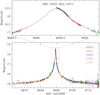 |
Fig. 7 Light curve of KMT-2022-BLG-0371. |
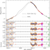 |
Fig. 8 Zoom of the central anomaly region of KMT-2022-BLG-0371. The lower five panels show the residuals from the four degenerate 2L1S (close A, B, C, and D solutions) and FSPL models. |
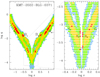 |
Fig. 9 ∆χ2 map constructed from the 2L1S modeling of KMT-2022-BLG-0371. The notations and color scheme of the plots are same as those of Fig. 3, except that n = 2. The locations of the four sets of local solutions are marked A, B, C, and D, and the subscripts c and w denote the close and wide solutions, respectively. |
3.4 KMT-2022-BLG-1013
The event KMT-2022-BLG-1013 occurred on a bulge star with coordinates (RA, Dec)J2000 = (17:38:50.22, −28:21:20.41), (l, b) = (−0°.291, 1°.570). It was detected in its early stage by the KMTNet survey on 2022 May 31 (HJD′ ~ 9729.7). The baseline magnitude registered in the DECam catalog is ibase = 21.31, and the extinction toward the field is A1 ~ 3.1. The source was in the KMTNet BLG14 field, toward which normal-mode observations were made with a 1.0 h cadence. At HJD′ = 9736.89, the KMTNet HighMagFinder system issued an alert that this event was peaking at a high magnification. Then, the peak region of the light curve was covered by the KMTS data with an intensified cadence of 0.12 hr during the period of 9737.30 ≤ HJD′ ≤ 9737.65, and additional data were acquired from follow-up observations conducted using the LCOC, LCOS, and Auckland telescopes.
The light curve of KMT-2022-BLG-1013 is presented in Fig. 12. To construct the light curve, we did not use the KMTA data set because its photometric quality was poor. In any case, there were no KMTA data taken near peak. The peak region appears to exhibit deviations caused by finite-source effects, and thus we first fit the light curve with an FSPL model. It is found that the FSPL model approximately describes the peak, but it leaves substantial positive residuals at a level of ~0. 1 mag in both the rising (9734 ≲ HJD′ ≲ 9736) and falling (9738 ≲ HJD′ ≲ 9740) sides, as shown in the bottom panel of Fig. 13.
From the thorough inspection of the parameter space, it is found that the residuals from the FSPL model are explained by a unique planetary model. Figure 14 shows the Δχ2 map obtained from the 2L1S grid searches for the binary-lens parameters s and q. We identify four local solutions, designated Sol Ac, Sol Aw, Sol B, and Sol C, and the locations of the individual locals are marked in the log s–log q parameter plane presented in Fig. 14. We note that the locals Sol Ac and Sol Aw are the pair of solutions resulting from the close-wide degeneracy. In Table 6, we list the refined lensing parameters of the individual local solutions, and the corresponding lens-system configurations are presented in the insets of the top panel of Fig. 13. We note that the Sol Ac and Sol Aw solutions result in similar configurations, and thus we present the configuration of the Sol Ac solution as the representative one. The residuals from the individual models are presented in the lower four panels of Fig. 13. From the comparison of the residuals and the χ2 values of the models, it is found that the Sol C model yields a substantially better fit to the data than the other models, by Δ χ2 = 42.8, 44.4, and 29.0 with respect to the Sol Ac, Sol Aw, and Sol B models, respectively. We also find that the Sol C model is preferred over the 1L2S model by Δ χ2 = 50.7.
According to the best-fit model, the mass ratio of the lens components is q ~ 1.6 × 10⁻³, indicating that the companion to the lens is a planet. The projected separation, s ~ 1.07, is very close to unity, and thus the planet induces a resonant caustic. The anomaly was produced by the successive caustic crossings of the source, which entered the caustic by crossing the upper fold of the caustic at HJD′ ~ 9734.6, passed through the inner caustic region, and then exited the caustic by going through the strong lower cusp of the caustic at HJD′ ~ 9738.9. According to the solution, the positive deviation in the rising part of the anomaly is explained by the source crossing over the upper fold caustic, and the positive deviation in the falling part is explained by the source passage through the positive anomaly region extending from the strong caustic cusp.
Model parameters of solutions A and B of KMT-2022-BLG-0371.
Model parameters of solutions C and D of KMT-2022-BLG-0371.
Proper motion probability for the four local solutions of KMT-2022-BLG-0371.
Model parameters of KMT-2022-BLG-1013.
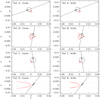 |
Fig. 10 Lens-system configurations of the four pairs of the local solutions of KMT-2022-BLG-0371. In each panel, the empty circle on the source trajectory represent the source size in units of the Einstein radius as given by the tick marks. |
4 Source stars and Einstein radii
In this section, we specify the source stars of the events. The main purpose of the source specification is estimating the angular Einstein radius of the planetary lens event from the measured normalized source radius by the relation

where the angular source radius θ* is deduced from the source type. We are able to measure the Einstein radii of the two events KMT-2022-BLG-0371 and KMT-2022-BLG-1013, for which the lenses are identified as planetary systems and the ρ values are measured. Although the lens of KMT-2021-BLG-2010 is a planetary system, the Einstein radius cannot be measured because the ρ value is not measured. In the case of KMT-2021-BLG-1968, the lens is not uniquely identified as a planetary system, and the ρ value is not measured either. Nevertheless, we specify the source stars of all events to fully characterize the lensing events.
We specified the source star of each event by measuring its dereddened color (V − I)S,0 and magnitude I0 using the routine of Yoo et al. (2004). Following the routine, we first measured the instrumental color and magnitude, (V − I,I)S, of the source, placed the source in the color-magnitude diagram (CMD) of stars around the source, measured the offset ∆(V − I,I) of the source position from the centroid of the red giant clump (RGC), with (V − I,I)RGC, in the CMD, and then estimated the dereddened source color and magnitude as

Here (V − I,I)RGC,0 denote the known values of the dereddened color and magnitude of the RGC centroid from Bensby et al. (2013) and Nataf et al. (2013), respectively. The instrumental source color was measured by regressing the I- and V-band photometry data with respect to the lensing magnification predicted by the model. In the cases of KMT-2021-BLG-1968 and KMT-2021-BLG-2010, for which the source stars are very faint, it was difficult to securely measure the V-band magnitudes. In this case, we used the CMD of Holtzman et al. (1998), which was constructed from the observations of bulge stars using the Hubble Space Telescope (HST), and interpolated the source color from the main-sequence branch on the HST CMD using the measured I-band magnitude difference between the source and RGC centroid.
Figure 15 shows the positions of the source stars and RGC centroids in the CMDs of the individual events. In Table 7 we list the values of (V − I, I)S, (V − I, I)S,0, (V − I, I)RGC, and (V − I, I)RGC,0 together with the stellar types determined from the dereddened color and magnitude. To estimate the angular source radius from (V − I, I)S,0, we first converted the V − I color into V − K color, and then deduced θ*. from the relation of Kervella et al. (2004) between (V − K, V) and θ*. The estimated source radii of the individual events are listed in Table 7.
With the measured source radius, we estimated the angular Einstein radii using the relation in Eq. (1). We also estimated the relative lens-source proper motion from the combination of the Einstein radius and event timescale by

In Table 8, we list the θΕ and µ values of the events for which the planetary nature of the lenses are identified.
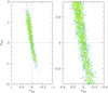 |
Fig. 11 Scatter plot of points in the MCMC chain on the πΕ,Ν−πΕ,Ε parameter plane of KMT-2022BLG-0371. The right panel shows the enlargement of the region around the origin. The color scheme of the plots is same as those of Fig. 3, except that n = 1. |
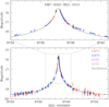 |
Fig. 12 Light curve of KMT-2022-BLG-1013. |
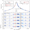 |
Fig. 13 Zoom of the central anomaly region of KMT-2022-BLG-1013. The lower five panels show the residuals from the three degenerate 2L1S (solutions A, B, and C), 1L2S, and FSPL models. The three insets in the top panel show the 2L1S lens-system configurations of solutions A, B, and C. |
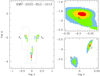 |
Fig. 14 Δχ2 map obtained from the 2L1S modeling of KMT-2022-BLG-1013. The notations and color scheme are same as those of Fig. 3, except that n = 2. |
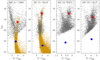 |
Fig. 15 Source locations (filled blue dots) of the events in the instrumental CMDs of stars around the source stars. In each panel, the filled red dot denotes the centroid of the red giant clump. |
Source stars.
Einstein radii and relative lens-source proper motions.
5 Physical parameters
In this section, we estimate the physical parameters of the three identified planetary lens systems of KMT-2021-BLG-2010L, KMT-2022-BLG-0371L, and KMT-2022-BLG-1013L. For none of these events, the lensing observables (tE, θΕ, πE) are fully measured, making it difficult to uniquely determine the mass M and distance DL to the planetary systems via the analytic relations

Here κ = 4G/(c2AU), πS = AU/DS denotes the parallax of the source, and DS represents the distance to the source. We therefore estimated the physical lens parameters by conducting Bayesian analyses based on the measured observables of the individual events.
The Bayesian analysis of each lensing event was carried out by conducting a Monte Carlo simulation of Galactic lensing events. From the simulation, we produced a large number (107) of lensing events, for which the locations of the lens and source and the relative proper motions were assigned based on a prior Galactic model, and the lens masses were allocated based on a prior mass function of Galactic objects. In the simulation, we adopted the Galactic model of Jung et al. (2021) and the mass function model of Jung et al. (2018). For each simulated event, we computed lensing observables by

where the relative parallax is defined as πrel = πL − πS = AU(1/DL − 1/DS). We then constructed posterior distributions of the physical parameters by imposing a weight wi = exp(−χ2 /2) to each simulated event. Here the χ2 value is computed as

where (tE,i, θE,i) represent the timescale and Einstein radius of each simulated event, and (tE, θE) denote the measured values. In the case of KMT-2021-BLG-2010, for which only the lower limit of θE is constrained, we set wi = 0 for simulated events with θE,i < θE,min. Although the constraint given by the measured microlens parallax parameters is weak in the case of KMT-2022-BLG-0371, we imposed the πE constraint by adding an additional term

to the right side of Eq. (6). Here bjk represents the inverse matrix of πE, (πE,1, πE,2)i = (πE,N, πE,E)i denote the parallax parameters of each simulated event, and (πE,N, πE,E) are the measured parallax parameters.
We present the posteriors of the mass and distance to the three planetary systems in Figs. 16 and 17, respectively. In Table 9, we list the estimated masses of the host, Mh, and planet, Mp, distance, DL, and projected separation of the planet from the host, a⊥ = sDLθE. For each parameter, we present the median as a representative value, and the uncertainties are estimated as 16% and 84% of the posterior distribution. For events with degenerate close and wide solutions, we present a pair of the projected separations resulting from the close and wide solutions. According to the estimated planet and host masses, the planetary system KMT-2021-BLG-2010L is composed of a Jupiter-mass planet and an M-dwarf host, the system KMT-2022-BLG-0371L consists of a sub-Iupiter-mass planet and a K-dwarf host, and the system KMT-2022-BLG-1013L is composed of a sub-Iupiter-mass planet and an M-dwarf host.
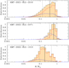 |
Fig. 16 Bayesian posteriors of the mass of the lens system for the planetary events KMT-2021-BLG-2010 and KMT-2022-BLG-1013. In each panel, the distributions drawn in red and blue represent the contributions of the bulge and disk lenses, respectively, and the distribution drawn in black is the sum of the contributions by the two lens populations. The solid vertical line indicates the median, and the dotted vertical lines represent 16% and 84% of the distribution. |
Physical lens parameters.
 |
Fig. 17 Bayesian posteriors of the distance to the lens system for the events KMT-2021-BLG-2010 and KMT-2022-BLG-1013. The notations are same as in Fig. 16. |
6 Summary and conclusion
We conducted analyses of four anomalous microlensing events detected in the 2021 and 2022 seasons, including KMT-2021-BLG-1968, KMT-2021-BLG-2010, KMT-2022-BLG-0371, and KMT-2022-BLG-1013. The light curves of the events commonly exhibit partially covered short-term central anomalies appearing near the highly magnified peaks. In order to reveal the nature of the anomalies, we tested various models that might explain the anomalies of the individual events, including the binary-lens and binary-source interpretations. Under the 2L1S interpretation, we thoroughly inspected the parameter space to verify the existence of degenerate solutions, and if they existed, we tested whether the degeneracy could be resolved.
We found that the anomalies of the two events KMT-2021-BLG-2010 and KMT-2022-BLG-1013 were uniquely explained by planetary-lens interpretations, for which the planet-to-host mass ratios are q ~ 2.8 × 10⁻³ and ~1.6 × 10⁻³, respectively. For KMT-2022-BLG-0371, we found multiple sets of local 2L1S solutions with different combinations of binary parameters, but a planetary solution with a mass ratio q ~ 4 × 10⁻⁴ was strongly preferred over the other degenerate solutions based on the χ2 and relative proper motion arguments, and a 1L2S solution was clearly ruled out. For KMT-2021-BLG-1968, on the other hand, it was found that the anomaly could be explained either by a planetary or by a binary-source interpretation, making it difficult to firmly identify the nature of the anomaly. From the Bayesian analyses of the identified planetary events, we estimated that the masses of the planet and host were,  , (
, ( ), and (
 ) for KMT-2021-BLG-2010L, KMT-2022-BLG-0371L, and KMT-2022-BLG-1013L, respectively.
Acknowledgements
Work by C.H. was supported by the grants of National Research Foundation of Korea (2019R1A2C2085965). J.C.Y., I.G.S, and S.J.C. acknowledge support from NSF Grant No. AST-2108414. W.Z. and H.Y. acknowledge the support by the National Science Foundation of China (Grant No. 12133005). Y.S. acknowledges support from BSF Grant No. 2020740. This research has made use of the KMTNet system operated by the Korea Astronomy and Space Science Institute (KASI) at three host sites of CTIO in Chile, SAAO in South Africa, and SSO in Australia. Data transfer from the host site to KASI was supported by the Korea Research Environment Open NETwork (KREONET). W. Zang, J.Z., H.Y., S.M., and W. Zhu acknowledge support by the National Natural Science Foundation of China (Grant No. 12133005). W. Zang acknowledges the support from the Harvard-Smithsonian Center for Astrophysics through the CfA Fellowship. This research uses data obtained through the Telescope Access Program (TAP), which has been funded by the TAP member institutes. W.Zhu acknowledges the science research grants from the China Manned Space Project with No. CMS-CSST-2021-A11. The authors acknowledge the Tsinghua Astrophysics High-Performance Computing platform at Tsinghua University for providing computational and data storage resources that have contributed to the research results reported within this paper.
References
- Alard, C., & Lupton, R. H. 1998, ApJ, 503, 325 [Google Scholar]
- Albrow, M., Horne, K., Bramich, D. M., et al. 2009, MNRAS, 397, 2099 [Google Scholar]
- An, J. H. 2005, MNRAS, 356, 1409 [Google Scholar]
- Bensby, T., Yee, J. C., Feltzing, S., et al. 2013, A & A, 549, A147 [NASA ADS] [CrossRef] [EDP Sciences] [Google Scholar]
- Chung, S.-J., Han, C., Park, B.-G., et al. 2005, ApJ, 630, 535 [Google Scholar]
- Dominik, M. 1999, A & A, 349, 108 [NASA ADS] [Google Scholar]
- Gould, A. 2022, ArXiv e-prints [arXiv:2209.12501] [Google Scholar]
- Griest, K., & Safizadeh, N. 1998, ApJ, 500, 37 [Google Scholar]
- Han, C. 2006, ApJ, 638, 1080 [Google Scholar]
- Han, C., & Hwang, K.-H. 2009, ApJ, 707, 1264 [NASA ADS] [CrossRef] [Google Scholar]
- Han, C., Lee, C.-U., Gould, A., et al. 2022a, A & A, 666, A132 [NASA ADS] [CrossRef] [EDP Sciences] [Google Scholar]
- Han, C., Udalski, A., Lee, C.-U., et al. 2022b, A & A, 658, A93 [NASA ADS] [CrossRef] [EDP Sciences] [Google Scholar]
- Holtzman, J. A., Watson, A. M., Baum, W. A., et al. 1998, AJ, 115, 1946 [Google Scholar]
- Hwang, K.-H., Choi, J.-Y., Bond, I., et al. 2013, ApJ, 778, 55 [NASA ADS] [CrossRef] [Google Scholar]
- Jung, Y. K., Udalski, A., Gould, A., et al. 2018, AJ, 155, 219 [Google Scholar]
- Jung, Y. K., Han, C., Udalski, A., et al. 2021, AJ, 161, 293 [NASA ADS] [CrossRef] [Google Scholar]
- Kervella, P., Thévenin, F., Di Folco, E., & Ségransan, D. 2004, A & A, 426, 29 [Google Scholar]
- Kim, S.-L., Lee, C.-U., Park, B.-G., et al. 2016, JKAS, 49, 37 [Google Scholar]
- Nataf, D. M., Gould, A., Fouqué, P., et al. 2013, ApJ, 769, 88 [Google Scholar]
- Schechter, P. L., Mateo, M., & Saha, A. 1993, PASP, 105, 1342 [Google Scholar]
- Tomaney, A. B., & Crotts, A. P. S. 1996, AJ, 112, 2872 [Google Scholar]
- Yang, H., Zang, W., Gould, A., et al. 2022, MNRAS, 5146, 189 [Google Scholar]
- Yee, J. C., Shvartzvald, Y., Gal-Yam, A., et al. 2012, ApJ, 755, 102 [Google Scholar]
- Yoo, J., DePoy, D. L., Gal-Yam, A., et al. 2004, ApJ, 603, 139 [Google Scholar]
- Zang, W., Han, C., Kondo, I., et al. 2021, Res. Astron. Astrophys., 21, 239 [CrossRef] [Google Scholar]
All Tables
All Figures
|
Fig. 1 Light curve of KMT-2021-BLG-1968. The lower panel shows the whole view, and the upper panel shows the enlarged view of the peak region around the anomaly. The 1L1S model curve is plotted over the data. |
| In the text | |
|
Fig. 2 Light curve of KMT-2021-BLG-1968 in the region of the anomaly. The curves drawn over the data points are 2L1S, 1L2S, and PSPL models, and the lower four panels show the residuals from the individual models. The three insets in the top panel show the lens-system configurations of the close and wide 2L1S solutions and the 1L2S solution. For each 2L1S configuration, the cuspy red figure represents the caustic, and the arrowed line indicates the source trajectory. For the 1L2S configuration, the small filled dot represents the lens position, and the arrowed lines marked in red and blue represent the trajectories of the primary and secondary source stars, respectively. |
| In the text | |
|
Fig. 3 ∆χ2 map on the (log s, log q) plane obtained from the 2L1S modeling of KMT-2021-BLG-1968. The right panel shows the enlargement of the map around the local minima. The colors represent points with ∆χ2 ≤ 1nσ (red), ≤ 2nσ (yellow), ≤ 3nσ (green), and ≤ 4nσ (cyan), where n = 3. |
| In the text | |
|
Fig. 4 Light curve of KMT-2021-BLG-2010. The layout and scheme of the plots are same as those of Fig. 1. |
| In the text | |
|
Fig. 5 Zoom of the central anomaly region of KMT-2021-BLG-2010. The lower four panels show the residuals from the close and wide 2L1S, 1L2S, and PSPL models. The two insets in the top panel show the lens-system configurations of the close and wide 2L1S solutions. |
| In the text | |
|
Fig. 6 ∆χ2 map from the 2L1S modeling of KMT-2021-BLG-2010. The notations and color scheme of the plots are same as those of Fig. 3, except that n = 2. |
| In the text | |
|
Fig. 7 Light curve of KMT-2022-BLG-0371. |
| In the text | |
|
Fig. 8 Zoom of the central anomaly region of KMT-2022-BLG-0371. The lower five panels show the residuals from the four degenerate 2L1S (close A, B, C, and D solutions) and FSPL models. |
| In the text | |
|
Fig. 9 ∆χ2 map constructed from the 2L1S modeling of KMT-2022-BLG-0371. The notations and color scheme of the plots are same as those of Fig. 3, except that n = 2. The locations of the four sets of local solutions are marked A, B, C, and D, and the subscripts c and w denote the close and wide solutions, respectively. |
| In the text | |
|
Fig. 10 Lens-system configurations of the four pairs of the local solutions of KMT-2022-BLG-0371. In each panel, the empty circle on the source trajectory represent the source size in units of the Einstein radius as given by the tick marks. |
| In the text | |
|
Fig. 11 Scatter plot of points in the MCMC chain on the πΕ,Ν−πΕ,Ε parameter plane of KMT-2022BLG-0371. The right panel shows the enlargement of the region around the origin. The color scheme of the plots is same as those of Fig. 3, except that n = 1. |
| In the text | |
|
Fig. 12 Light curve of KMT-2022-BLG-1013. |
| In the text | |
|
Fig. 13 Zoom of the central anomaly region of KMT-2022-BLG-1013. The lower five panels show the residuals from the three degenerate 2L1S (solutions A, B, and C), 1L2S, and FSPL models. The three insets in the top panel show the 2L1S lens-system configurations of solutions A, B, and C. |
| In the text | |
|
Fig. 14 Δχ2 map obtained from the 2L1S modeling of KMT-2022-BLG-1013. The notations and color scheme are same as those of Fig. 3, except that n = 2. |
| In the text | |
|
Fig. 15 Source locations (filled blue dots) of the events in the instrumental CMDs of stars around the source stars. In each panel, the filled red dot denotes the centroid of the red giant clump. |
| In the text | |
|
Fig. 16 Bayesian posteriors of the mass of the lens system for the planetary events KMT-2021-BLG-2010 and KMT-2022-BLG-1013. In each panel, the distributions drawn in red and blue represent the contributions of the bulge and disk lenses, respectively, and the distribution drawn in black is the sum of the contributions by the two lens populations. The solid vertical line indicates the median, and the dotted vertical lines represent 16% and 84% of the distribution. |
| In the text | |
|
Fig. 17 Bayesian posteriors of the distance to the lens system for the events KMT-2021-BLG-2010 and KMT-2022-BLG-1013. The notations are same as in Fig. 16. |
| In the text | |
Current usage metrics show cumulative count of Article Views (full-text article views including HTML views, PDF and ePub downloads, according to the available data) and Abstracts Views on Vision4Press platform.
Data correspond to usage on the plateform after 2015. The current usage metrics is available 48-96 hours after online publication and is updated daily on week days.
Initial download of the metrics may take a while.