| Issue |
A&A
Volume 668, December 2022
|
|
|---|---|---|
| Article Number | A9 | |
| Number of page(s) | 7 | |
| Section | The Sun and the Heliosphere | |
| DOI | https://doi.org/10.1051/0004-6361/202244427 | |
| Published online | 28 November 2022 | |
Statistical analysis of the Si I 6560.58 Å line observed by CHASE⋆
1
School of Astronomy and Space Science, Nanjing University, Nanjing 210023, PR China
e-mail: jiehong@nju.edu.cn
2
Key Laboratory for Modern Astronomy and Astrophysics (Nanjing University), Ministry of Education, Nanjing 210023, PR China
3
Yunnan Observatories, Chinese Academy of Sciences, Kunming 650216, PR China
Received:
6
July
2022
Accepted:
27
September
2022
Context. The Si I 6560.58 Å line in the Hα blue wing is blended with a telluric absorption line from water vapor in ground-based observations. Recent observations with the space-based telescope, the Chinese Hα Solar Explorer (CHASE), provide a new opportunity to study this line.
Aims. We aim to study the Si I line statistically and to explore possible diagnostics.
Methods. We selected three scannings in the CHASE observations, and measured the equivalent width (EW) and the full width at half maximum (FWHM) for each pixel on the solar disk. We then calculated the theoretical EW and FWHM from the VALC model. We also studied an active region in particular in order to identify possible differences in the quiet Sun and the sunspots.
Results. The Si I line is formed at the bottom of the photosphere. The EW of this line increases from the disk center to μ = 0.2, and then decreases toward the solar limb, while the FWHM shows a monotonically increasing trend. Theoretically predicted EW agrees well with observations, while the predicted FWHM is far smaller due to the absence of unresolved turbulence in models. The macroturbulent velocity is estimated to be 2.80 km s−1 at the disk center, and increases to 3.52 km s−1 at μ = 0.2. We do not find any response to flare heating in the observations studied here. Doppler shifts and line widths of the Si I 6560.58 Å and Fe I 6569.21 Å lines can be used to study the mass flows and turbulence of the different photospheric layers. The Si I line shows significant potential as a tool to diagnose the dynamics and energy transport in the photosphere.
Key words: line: formation / line: profiles / Sun: photosphere / turbulence
Data are also available at the CDS via anonymous ftp to cdsarc.cds.unistra.fr (130.79.128.5) or via https://cdsarc.cds.unistra.fr/viz-bin/cat/J/A+A/668/A9
© J. Hong et al. 2022
 Open Access article, published by EDP Sciences, under the terms of the Creative Commons Attribution License (https://creativecommons.org/licenses/by/4.0), which permits unrestricted use, distribution, and reproduction in any medium, provided the original work is properly cited.
This article is published in open access under the Subscribe-to-Open model. Subscribe to A&A to support open access publication.
1. Introduction
The solar photosphere is home to the abundant metal lines that appear absorptive against the optical continuum background. These lines contain rich information about the photosphere and have been extensively studied over the last century. Most studies are devoted to the determination of element abundances from the equivalent widths of these absorption lines (e.g., Asplund et al. 2021). Micro- and macroturbulent velocities can also be obtained from the equivalent widths (EWs) or line profiles (Takeda 1995, 2022; Sheminova 2019).
Transitions between the Si I 3p4p 3D1, 2, 3 and 3p7d 3 levels give rise to six allowed lines in the visible waveband, and one of them resides at the Hα blue wing, with a wavelength of 6560.58 Å (Radziemski & Andrew 1965; Lambert & Warner 1968). This line has been identified in previous solar atlases as blended with another telluric absorption line from water vapor (Moore et al. 1966; Delbouille et al. 1973). The Kitt Peak solar atlas unveiled this line for the first time after a careful evaluation of the atmospheric transmission spectra (Kurucz et al. 1984). However, in spite of the only record of the EW value in the past literature (Moore et al. 1966; Lambert & Warner 1968), information about this line is still scarce due to line blending.
The Chinese Hα Solar Explorer (CHASE, Li et al. 2019, 2022) is a space-based telescope that can perform spectroscopic observations of the full solar disk in the Hα waveband. The absorptive Si I 6560.58 Å line clearly stands out in the sample spectra (Qiu et al. 2022), without any distortion or disturbance from the Earth’s atmosphere, making its study feasible.
In this paper, we use full-disk spectra of the Si I 6560.58 Å line and investigate its formation and its diagnosing potentials of the solar photosphere. We briefly introduce our observations and data reduction methods in Sect. 2. The results are shown in Sect. 3, followed by our conclusions in Sect. 4.
2. Observations and data reduction
CHASE1 can regularly scan the full solar disk in both the Hα and Fe I wavebands. Each scanning takes ∼46 s, with a spectral sampling of 24.2 mÅ. After in-orbit focus calibration at the beginning of August 2022, a spatial resolution of 1 2 was achieved. Normally, a 2× binning is used to reduce the data size. We chose three full-Sun observation periods, all with flares in the northern hemisphere. The selected scanning in each observation period is closest to the flare peak time, as listed in Table 1. The selected scanning OBS1 is near the flare peak time, while OBS2 is in the pre-flare phase and OBS3 is in the decay phase. We show the reconstructed images at the Si I and Hα line centers in Fig. 1, and note that part of the solar disk in OBS1 is outside the field of view. The signal-to-noise ratio (S/N) is calculated in the Hα far wings, and expressed in units of decibels (dB).
Basic information of the selected full-Sun scannings.
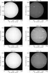 |
Fig. 1. Reconstructed images at the Si I and Hα line centers. |
As shown in Qiu et al. (2022), the enhancement of the observed line center is mainly due to the contamination of stray light (Fig. 2). Following Hou et al. (2020), the level of stray light is estimated by least-square fitting the observed profile at disk center with the convolved standard profile of BASS20002 (Delbouille et al. 1973). The spectra are then corrected assuming that the influence of stray light is constant over the full field of view, and we show the corrected disk-center sample spectra in Fig. 2. We determined the solar disk center and radius from the reconstructed Hα line wing image using the method proposed by Hao et al. (2015).
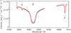 |
Fig. 2. Sample disk-center spectra with identified lines from the CHASE Hα and Fe I wavebands after radiometric calibration. The black curve is the original spectra, and the red one is after stray-light correction. |
3. Results
3.1. Line formation
We use the RH code (Uitenbroek 2001; Pereira & Uitenbroek 2015) to calculate the line profiles of the quiet-sun VALC model (Vernazza et al. 1981) while assuming no turbulent velocity, no line-of-sight velocity, and no magnetic field. The Hα line is calculated in nonlocal thermodynamic equilibrium (non-LTE), while the superposed Si I 6560.58 Å and Fe I 6569.21 Å lines are treated in LTE, with their data from the Kurucz line database (Kurucz 2018). We calculate the line profiles from the solar disk center to the solar limb, with the cosine of heliocentric angle μ varying from 1.0 to 0.05.
The contribution function is defined as CI(z)=jνexp(−τν), where jν is the emissivity and τν is the optical depth, and an integration along the height z gives the value of emergent intensity. Figure 3 shows the contribution functions at the line center of the Si I 6560.58 Å and Fe I 6569.21 Å lines. Both lines are formed in the optically thick regime, because the contribution function peaks below the τ = 1 height. The formation height is defined as the centroid of the contribution function, and is marked with a dashed vertical line. The Fe I line forms in the mid-photosphere (around 250 km), similar to other Fe I lines that are sensitive to magnetic fields (Shchukina & Trujillo Bueno 2001; Hong et al. 2018). The Si I line forms much lower than the Fe I line, almost at the bottom of the photosphere (around 70 km). The low formation height of the Si I line also justifies the LTE assumption, which means that we are not forced to deal with the complicated Si model atom, as in Bard & Carlsson (2008).
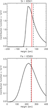 |
Fig. 3. Contribution functions at the line center of the Si I 6560.58 Å and Fe I 6569.21 Å lines. Black vertical lines marks the formation height, and red vertical lines denote the height where τ = 1. |
3.2. Center-to-limb variation
3.2.1. Equivalent width
The EW of an absorption line is defined as the integration of the normalized line depth profile over wavelength:
For all these three observations, we calculate the values of EW for each pixel on the solar disk. Data pixels at the solar limb where μ < 0.15 are discarded because this line becomes relatively weak. We also calculate the EWs from the VALC model for μ = 1.0 until μ = 0.05.
The probability density functions of the EW as a function of μ in the three observations are shown in Fig. 4 in grayscale. The average value and 1σ range at each μ are overplotted as red and blue curves, while the calculated values from the VALC model are shown as green diamonds. These values are also listed in Table 2 for comparison.
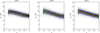 |
Fig. 4. Probability density function of the EW of the Si I line as a function of the cosine of the heliocentric angle. Red and blue lines show the averaged value and 1σ range, and the green diamonds show the calculated values from the VALC model with no turbulent velocity. |
Center-to-limb distribution of the EW and the FWHM of the Si I line from model calculations and observed mean values.
It is clear that the center-to-limb variation of EW as revealed from the three observations is quite similar, and agrees well with model calculations. Generally speaking, the EW increases from center to limb, and reaches its peak value near μ = 0.2, and then begins to decrease. The variation of the EW could be interpreted in the following way. As μ increases, both the Si I line and the continuum are formed in higher layers with a lower local temperature, leading to a decrease in both the line and the continuum intensity. A smaller line intensity tends to increase the EW, while a smaller continuum intensity tends to decrease the EW. As the line and continuum are formed at different heights, the decreasing percentage of their intensity at a certain μ could vary. The competition of these two factors leads to the final results: when μ decreases from 1.0 to 0.2, the line intensity decreases more sharply than the continuum; while the decrease in continuum dominates for μ < 0.2. The differences between the average values from observations and the calculated values from models are less than 1 mÅ, which is within the 1σ range.
The only recorded EW value for this line in the literature is from the revised Rowland Table by Moore et al. (1966), which reads 22 mÅ at the disk center. We also measure the EW from the Jungfraujoch atlas (BASS2000, Delbouille et al. 1973) and the Kitt Peak atlas (Kurucz et al. 1984), and they give values of 18.52 and 17.27 mÅ, respectively, at the disk center. All these values are far larger than the observed values from CHASE, even outside the 1σ range, which is mostly due to the fact that the Si I line is blended with a telluric absorption line. Although the Kitt Peak atlas has corrected the atmospheric transmission, it seems that their evaluation is still not accurate.
3.2.2. Full width at half maximum
The full width at half maximum (FWHM) of an absorption profile is determined by various line-broadening mechanisms, and is close to the FWHM of the line profile in the optically thin regime. For optically thick lines, the FWHMs of the line profile and the absorption profile are not necessarily the same due to the so-called opacity broadening (Rathore & Carlsson 2015), while they are still positively related. Here, we measure the FWHM of the line depth profile Rλ for each pixel on the solar disk where μ ≥ 0.15. We note that the observed profiles are not corrected with a deconvolution of the instrumental profile. Thus, the measured FWHM has included the instrumental FWHM of 72.6 mÅ (Li et al. 2022).
In Fig. 5 we show the probability density functions of the FWHM as a function of μ in the three observations. Despite the spikes and substructures, there is still an increasing trend for the FWHM from the disk center to the solar limb. However, the calculated FWHM from the VALC model after convolution with the CHASE instrumental profile – as denoted by green diamonds and also listed in Table 2 – is quite different from the observed values. Without any turbulent velocities, the calculated FWHM decreases toward the solar limb, because for a smaller μ, the line forms higher in the photosphere where the lower temperature narrows the thermal width. For comparison, the measured FWHM is 166 mÅ from the Jungfraujoch atlas (BASS2000, Delbouille et al. 1973) and 158 mÅ from the Kitt Peak atlas (Kurucz et al. 1984), after convolution with the CHASE instrumental profile. The discrepancy of observed and calculated FWHM values are explained below.
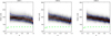 |
Fig. 5. Same as Fig. 4, but for the FWHM of the Si I line. An instrumental FWHM of 72.6 mÅ is included. |
3.2.3. Micro- and macroturbulent velocities
Traditionally, nonthermal turbulent velocities are introduced to explain the excess width in the absorption profiles and line profiles. A dichotomy of microturbulence and macroturbulence is employed from the geometric scale of the motions. Microturbulence occurs within the mean free path of photons, and so the line absorption is changed, resulting in larger EW and FWHM. However, macroturbulence does not influence the line absorption and only broadens the line profile.
We recalculate the EW of the Si I line assuming different values of microturbulent velocity in the VALC model. The results for the μ = 0.6 case are shown in Fig. 6. The value of μ = 0.6 is chosen arbitrarily here for illustration, and the increasing trend is similar for other values of μ. One can see that the EW increases by 1.1 mÅ for a microturbulent velocity of 4 km s−1. Given the large uncertainties in the EW measurement from the observations, any derivation of the microturbulent velocities would be unreliable.
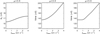 |
Fig. 6. Calculated EW and FWHM from the VALC model with different micro- and macroturbulent velocities. An instrumental FWHM of 72.6 mÅ is included. |
As stated above, the FWHM of an absorption line is influenced by both micro- and macroturbulent velocities, and Fig. 6 provides a schematic view of their contributions as calculated from the VALC model. The line profile has been convolved with the CHASE instrumental profile in order to compare with observations. The macroturbulent velocity is then added by convolving the line depth profile with a Gaussian velocity distribution:
As shown in Fig. 6, both turbulent velocities could effectively increase the FWHM. However, the increase in the FWHM is not obvious for small macroturbulent velocities under the spectral resolution of CHASE.
In order to separate the contributions from micro- and macroturbulent velocities to the FWHM, we fix the values for microturbulent velocities at different positions on the solar disk. We take the empirical formula of Takeda (2022), which shows an increasing trend of the microturbulent velocities toward the solar limb, with 1 km s−1 at the disk center and 1.97 km s−1 at μ = 0.2. The macroturbulent velocities are then derived from a similar relation as in Fig. 6 after inclusion of the microturbulent velocities. The results from the three observations are shown in Fig. 7. There is also an increasing trend toward the solar limb, with 2.80 km s−1 at the disk center and 3.52 km s−1 at μ = 0.2. The center-to-limb variation of the macroturbulent velocity can be interpreted as the intrinsic anisotropy of photospheric motions. If we consider a radial turbulent velocity ξr and a tangential turbulent velocity ξt, then the total macroturbulent velocity would be  (Takeda & UeNo 2017). A least-square fit to the averaged values in our observations (Fig. 7) gives ξr = 2.85 km s−1 and ξt = 3.58 km s−1. These values are slightly larger than previous ones derived from the Fe I lines (Takeda & UeNo 2017; Sheminova 1985), because the Si I line forms deeper in the photosphere where the unresolved turbulent motions are faster, as revealed from observations and simulations (Gray 1977, 1978; Takeda 1995; Beeck et al. 2012; Takeda & UeNo 2017).
 |
Fig. 7. Center-to-limb variations of the macroturbulent velocities derived from observations. A fitted curve with ξr = 2.85 km s−1 and ξt = 3.58 km s−1 is overplotted. |
3.3. Variations in an active region
The magnetic structure of an active region is apparently different from that of the quiet Sun, leading to a different atmospheric structure and thus a different line profile. We select the active region in the northern hemisphere in OBS1 with a field of view of 300 pixels × 300 pixels (∼312″ × 312″), where the C2.5 flare is near its peak time. One can clearly identify the sunspot group in the intensity map of Si I, and the flare kernel in the intensity map of Hα (Fig. 8a,b). We fit the Si I and Fe I line profiles using a Gaussian function with a slanted background:

where A0 is the line center depth, A1 is the observed line center, and A2 is the line width. The reference line center is chosen as the averaged A1 of the uppermost quiet region in the field of view. The line width A2 is positively related to the FWHM.
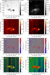 |
Fig. 8. Reconstructed maps from the spectra and fitting parameters. (a)–(b) Intensity maps of the Si I and Hα line center. The arrow points to disk center. The red plus symbols denote positions whose line profiles are shown in Fig. 9. (c)–(d) Line-center depth maps of the Si I and Fe I line. (e)–(f) Doppler maps of the Si I and Fe I line. (g)–(h) Line-width maps of the Si I and Fe I line. |
The reconstructed maps of the fitting parameters are shown in Fig. 8, and the line profiles of selected positions are shown in Figs. 9a,b. The line-center depth of the Fe I line is generally larger than that of the Si I line, and the values at the sunspots are smaller than the values at the quiet Sun (Figs. 8c,d). We also show the line profiles of the flare kernel at different times in Figs. 9c,d. We do not find any enhancement of these two lines as a response to flare heating, as judged from the variation of line profiles with time. Given the fact that the Si I line forms in the deep photosphere, either extremely energetic nonthermal particles or local reconnections are expected to heat the photosphere and give rise to its intensity. However, the Doppler maps show interesting outflows in the sunspot penumbra, with velocities of less than 2 km s−1 (Figs. 8e,f), known as the Evershed flows. The outflows revealed from the Si I line are larger than those from the Fe I line, with a velocity ratio in the range of 1.5–1.9, indicating a decrease in the flow velocities at greater heights, which agrees with previous inversions and simulations (Siu-Tapia et al. 2017, 2018). The Si I line width is also larger than the Fe I line width, which is attributed to both a larger thermal width and a larger turbulent velocity at smaller heights.
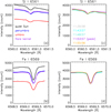 |
Fig. 9. Line profiles at different locations. (a)–(b) Sample line profiles at selected points in different regions (marked with plus symbols in Fig. 8). (c)–(d) Line profiles of the flare kernel at selected time. |
Histograms of the Si I line-center intensity, EW, and FWHM for different regions are shown in Fig. 10. No obvious difference is found for the EW in different regions. This implies that although the local temperature varies from region to region, the ratio of line intensity to continuum intensity are still in the same range. However, the FWHMs in sunspot areas are generally larger than those in the quiet Sun, which has been observed previously (Moore et al. 1966), indicating larger unresolved turbulent velocities in sunspots.
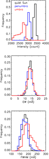 |
Fig. 10. Histograms of Si I line-center intensity, EW, and FWHM for different regions. |
3.4. Diagnosing potentials
Due to the low formation height, the Si I line is able to unveil the motions and turbulences in the deep photosphere. By combination with other photospheric lines, such as the Fe I line, which is simultaneously observed by CHASE, a full picture of the velocity field in the photosphere could be reconstructed. It would therefore be more feasible to catch the initial process of flux emergence, as well as the formation of active regions (Chen et al. 2022) and following activities, such as the Evershed flows inside the magnetic flux tubes (Murabito et al. 2016; Siu-Tapia et al. 2017, 2018). In addition, the full-disk velocity map at different atmospheric layers could be used to measure the solar differential rotation, providing new restrictions to the solar dynamo theory (Beck 2000).
The enhancement of the Si I line center intensity usually characterizes local heating in the formation height. Whether or not the deep photosphere could be effectively heated remains to be investigated with further observational evidence. Possible candidates of heating mechanisms include local magnetic reconnections (Chen et al. 2001; Song et al. 2020) and extremely energetic particles (Xu et al. 2006; Hong et al. 2018; Kowalski et al. 2019). Cross-correlations of the Si I intensity maps could also reveal possible helioseismic waves that could be evidence of local disturbance in the lower photosphere (Zhao et al. 2011).
4. Conclusion
In this paper, we present a statistical analysis of the Si I 6560.58 Å line observed with CHASE, which is free from line blending. The Si I line is formed at the bottom of the photosphere, which is even lower than the simultaneously observed Fe I 6569.21 Å line. The measured EW of the Si I line increases from the disk center until μ = 0.2, and then decreases toward the solar limb, reflecting the variation of the decreasing percentages of line intensity and continuum intensity. The theoretical calculation of the center-to-limb variation of the EW from the VALC model generally agrees well with the observations. However, the FWHM shows a monotonically increasing trend from center to limb which is far from model predictions. The discrepancy can be attributed to the unresolved macroscopic turbulent motions in the photosphere. The macroturbulent velocity is derived to be 2.80 km s−1 at disk center, and increases to 3.52 km s−1 at μ = 0.2. The center-to-limb variation of the macroturbulent velocity indicates the anisotropy of photospheric motions, which requires future observations from other photospheric lines in order to reconstruct the full physical picture of the photosphere.
In our observations, neither the Si I nor the Fe I line shows any response to flare heating. The Doppler maps of these lines show indications of Evershed flows in the sunspot penumbra. The line width and Doppler velocity from the Si I line are generally larger than those from the Fe I line, which is because the lower layers are more turbulent and have a higher temperature. While the FWHMs in sunspot areas are generally larger than in the quiet Sun, the EWs from these regions do not show obvious differences. This indicates larger unresolved turbulent velocities in sunspot areas, while the line-to-continuum intensity ratio stays in the same range. As routinely observed by CHASE, these lines provide a promising tool with which to study the mass flows and turbulence in the different photospheric layers, especially those connected to differential rotation or flux emergence. The deeply formed Si I line, when combined with other photospheric lines, also shows good potential in the diagnostics of energy
transport in the photosphere, such as white-light flares and helioseismic waves.
Acknowledgments
We are grateful to the referee for constructive comments. J.H. would like to thank Yikang Wang for fruitful discussions. The CHASE mission is supported by China National Space Administration. This work was supported by National Key R&D Program of China under grant 2021YFA1600504 and by NSFC under grants 11903020, 11733003, 12127901, and 11873091.
References
- Asplund, M., Amarsi, A. M., & Grevesse, N. 2021, A&A, 653, A141 [NASA ADS] [CrossRef] [EDP Sciences] [Google Scholar]
- Bard, S., & Carlsson, M. 2008, ApJ, 682, 1376 [NASA ADS] [CrossRef] [Google Scholar]
- Beck, J. G. 2000, Sol. Phys., 191, 47 [NASA ADS] [CrossRef] [Google Scholar]
- Beeck, B., Collet, R., Steffen, M., et al. 2012, A&A, 539, A121 [NASA ADS] [CrossRef] [EDP Sciences] [Google Scholar]
- Chen, P.-F., Fang, C., & Ding, M.-D. D. 2001, Chin. J. Astron. Astrophys., 1, 176 [NASA ADS] [CrossRef] [Google Scholar]
- Chen, F., Rempel, M., & Fan, Y. 2022, ApJ, 937, 2 [NASA ADS] [CrossRef] [Google Scholar]
- Delbouille, L., Roland, G., & Neven, L. 1973, Atlas photometrique du spectre solaire de [lambda] 3000 a [lambda] 10000 (Liége: Université de Liége) [Google Scholar]
- Gray, D. F. 1977, ApJ, 218, 530 [NASA ADS] [CrossRef] [Google Scholar]
- Gray, D. F. 1978, Sol. Phys., 59, 193 [NASA ADS] [CrossRef] [Google Scholar]
- Hao, Q., Fang, C., Cao, W., & Chen, P. F. 2015, ApJS, 221, 33 [NASA ADS] [CrossRef] [Google Scholar]
- Hong, J., Ding, M. D., Li, Y., & Carlsson, M. 2018, ApJ, 857, L2 [NASA ADS] [CrossRef] [Google Scholar]
- Hou, J.-F., Xu, Z., Yuan, S., et al. 2020, Res. Astron. Astrophys., 20, 045 [CrossRef] [Google Scholar]
- Kowalski, A. F., Butler, E., Daw, A. N., et al. 2019, ApJ, 878, 135 [NASA ADS] [CrossRef] [Google Scholar]
- Kurucz, R. L. 2018, in Workshop on Astrophysical Opacities, ASP Conf. Ser., 515, 47 [NASA ADS] [Google Scholar]
- Kurucz, R. L., Furenlid, I., Brault, J., & Testerman, L. 1984, Solar flux atlas from 296 to 1300 nm (New Mexico: National Solar Observatory) [Google Scholar]
- Lambert, D. L., & Warner, B. 1968, MNRAS, 139, 35 [NASA ADS] [CrossRef] [Google Scholar]
- Li, C., Fang, C., Li, Z., et al. 2019, Res. Astron. Astrophys., 19, 165 [CrossRef] [Google Scholar]
- Li, C., Fang, C., Li, Z., et al. 2022, Sci. China-Phys. Mech. Astron., 65, 289602 [NASA ADS] [CrossRef] [Google Scholar]
- Moore, C. E., Minnaert, M. G. J., & Houtgast, J. 1966, The Solar Spectrum 2935 A to 8770 A (Washington: US Government Printing Office) [Google Scholar]
- Murabito, M., Romano, P., Guglielmino, S. L., Zuccarello, F., & Solanki, S. K. 2016, ApJ, 825, 75 [NASA ADS] [CrossRef] [Google Scholar]
- Pereira, T. M. D., & Uitenbroek, H. 2015, A&A, 574, A3 [NASA ADS] [CrossRef] [EDP Sciences] [Google Scholar]
- Qiu, Y., Rao, S., Li, C., et al. 2022, Sci. China-Phys. Mech. Astron., 65, 289603 [NASA ADS] [CrossRef] [Google Scholar]
- Radziemski, L. J., & Andrew, K. L. 1965, J. Opt. Soc. Am., 55, 474 [NASA ADS] [CrossRef] [Google Scholar]
- Rathore, B., & Carlsson, M. 2015, ApJ, 811, 80 [NASA ADS] [CrossRef] [Google Scholar]
- Shchukina, N., & Trujillo Bueno, J. 2001, ApJ, 550, 970 [NASA ADS] [CrossRef] [Google Scholar]
- Sheminova, V. A. 1985, Kinematics Phys. Celestial Bodies, 1, 50 [Google Scholar]
- Sheminova, V. A. 2019, Kinematics Phys. Celestial Bodies, 35, 129 [NASA ADS] [CrossRef] [Google Scholar]
- Siu-Tapia, A., Lagg, A., Solanki, S. K., van Noort, M., & Jurčák, J. 2017, A&A, 607, A36 [NASA ADS] [CrossRef] [EDP Sciences] [Google Scholar]
- Siu-Tapia, A. L., Rempel, M., Lagg, A., & Solanki, S. K. 2018, ApJ, 852, 66 [Google Scholar]
- Song, Y., Tian, H., Zhu, X., et al. 2020, ApJ, 893, L13 [NASA ADS] [CrossRef] [Google Scholar]
- Takeda, Y. 1995, PASJ, 47, 337 [NASA ADS] [Google Scholar]
- Takeda, Y. 2022, Sol. Phys., 297, 4 [NASA ADS] [CrossRef] [Google Scholar]
- Takeda, Y., & UeNo, S. 2017, PASJ, 69, 46 [NASA ADS] [Google Scholar]
- Uitenbroek, H. 2001, ApJ, 557, 389 [Google Scholar]
- Vernazza, J. E., Avrett, E. H., & Loeser, R. 1981, ApJS, 45, 635 [Google Scholar]
- Xu, Y., Cao, W., Liu, C., et al. 2006, ApJ, 641, 1210 [NASA ADS] [CrossRef] [Google Scholar]
- Zhao, J., Kosovichev, A. G., & Ilonidis, S. 2011, Sol. Phys., 268, 429 [NASA ADS] [CrossRef] [Google Scholar]
All Tables
Center-to-limb distribution of the EW and the FWHM of the Si I line from model calculations and observed mean values.
All Figures
|
Fig. 1. Reconstructed images at the Si I and Hα line centers. |
| In the text | |
|
Fig. 2. Sample disk-center spectra with identified lines from the CHASE Hα and Fe I wavebands after radiometric calibration. The black curve is the original spectra, and the red one is after stray-light correction. |
| In the text | |
|
Fig. 3. Contribution functions at the line center of the Si I 6560.58 Å and Fe I 6569.21 Å lines. Black vertical lines marks the formation height, and red vertical lines denote the height where τ = 1. |
| In the text | |
|
Fig. 4. Probability density function of the EW of the Si I line as a function of the cosine of the heliocentric angle. Red and blue lines show the averaged value and 1σ range, and the green diamonds show the calculated values from the VALC model with no turbulent velocity. |
| In the text | |
|
Fig. 5. Same as Fig. 4, but for the FWHM of the Si I line. An instrumental FWHM of 72.6 mÅ is included. |
| In the text | |
|
Fig. 6. Calculated EW and FWHM from the VALC model with different micro- and macroturbulent velocities. An instrumental FWHM of 72.6 mÅ is included. |
| In the text | |
|
Fig. 7. Center-to-limb variations of the macroturbulent velocities derived from observations. A fitted curve with ξr = 2.85 km s−1 and ξt = 3.58 km s−1 is overplotted. |
| In the text | |
|
Fig. 8. Reconstructed maps from the spectra and fitting parameters. (a)–(b) Intensity maps of the Si I and Hα line center. The arrow points to disk center. The red plus symbols denote positions whose line profiles are shown in Fig. 9. (c)–(d) Line-center depth maps of the Si I and Fe I line. (e)–(f) Doppler maps of the Si I and Fe I line. (g)–(h) Line-width maps of the Si I and Fe I line. |
| In the text | |
|
Fig. 9. Line profiles at different locations. (a)–(b) Sample line profiles at selected points in different regions (marked with plus symbols in Fig. 8). (c)–(d) Line profiles of the flare kernel at selected time. |
| In the text | |
|
Fig. 10. Histograms of Si I line-center intensity, EW, and FWHM for different regions. |
| In the text | |
Current usage metrics show cumulative count of Article Views (full-text article views including HTML views, PDF and ePub downloads, according to the available data) and Abstracts Views on Vision4Press platform.
Data correspond to usage on the plateform after 2015. The current usage metrics is available 48-96 hours after online publication and is updated daily on week days.
Initial download of the metrics may take a while.