| Issue |
A&A
Volume 666, October 2022
|
|
|---|---|---|
| Article Number | A145 | |
| Number of page(s) | 22 | |
| Section | Extragalactic astronomy | |
| DOI | https://doi.org/10.1051/0004-6361/202243678 | |
| Published online | 19 October 2022 | |
A bottom-up search for Lyman-continuum leakage in the Hubble Ultra Deep Field
The Oskar Klein Centre, Department of Astronomy, Stockholm University, AlbaNova, 10691 Stockholm, Sweden
e-mail: trive@astro.su.se
Received:
30
March
2022
Accepted:
2
August
2022
Context. When studying the production and escape of Lyman continuum (LyC) from galaxies, it is standard to rely on an array of indirect observational tracers in the preselection of candidate leakers.
Aims. In this work, we investigate how much ionizing radiation might be missed due to these selection criteria by completely removing them and performing a search selected purely from rest-frame LyC emission; and how that affects our estimates of the ionizing background.
Methods. We inverted the conventional method and performed a bottom-up search for LyC leaking galaxies at redshifts 2 ≲ z ≲ 3.5. Using archival data from HST and VLT/MUSE, we ran source finding software on UV-filter HST images from the Hubble Ultra Deep Field (HUDF), and subjected all detected sources to a series of tests to eliminate those that are inconsistent with being ionizing sources.
Results. We find six new and one previously identified candidate leakers with absolute escape fractions ranging from 36% to ∼100%. Our filtering criteria eliminate one object previously reported as a candidate ionizing emitter in the literature, and we report non-detections in the rest-frame Lyman continuum of two other previously reported sources. We find that our candidates make a contribution to the metagalactic ionizing field of log10(ϵν) = 25.32−0.21+0.25 and 25.29−0.22+0.27 erg s−1 Hz−1 cMpc−3 for the full set of candidates and for the four strongest candidates only; both values are higher than but consistent with other recent figures in the literature.
Conclusions. Our findings suggest that galaxies that do not meet the usual selection criteria may make a non-negligible contribution to the cosmic ionizing field. We recommend that similar searches be carried out on a larger scale in well-studied fields with both UV and large ancillary data coverage, for example in the full set of CANDELS fields.
Key words: dark ages, reionization, first stars / galaxies: ISM / galaxies: evolution / galaxies: general
© T. E. Rivera-Thorsen et al. 2022
 Open Access article, published by EDP Sciences, under the terms of the Creative Commons Attribution License (https://creativecommons.org/licenses/by/4.0), which permits unrestricted use, distribution, and reproduction in any medium, provided the original work is properly cited.
This article is published in open access under the Subscribe-to-Open model. Subscribe to A&A to support open access publication.
1. Introduction
The Epoch of Reionization (EoR) was the last major phase transition of the Universe and ended around z ∼ 5.5–6 (e.g., Fan et al. 2006; Dayal et al. 2020; Bosman et al. 2022). At the relevant redshifts, the cosmic active galactic nucleus (AGN) population was probably still too low to dominate the metagalactic ionizing radiation (e.g., Haardt & Madau 2012; Faucher-Giguère 2020; Madau & Haardt 2015). Young, hot stars in star-forming galaxies thus most likely contributed the bulk of ionizing photons. The balancing of the budget of ionizing photons required to account for reionization is still an ongoing topic of research. The amount of ionizing photons required to account for reionization is still debated (e.g., Davies et al. 2021), as is the timescale and thus the required photon production rate (e.g., Naidu et al. 2020; Becker et al. 2021, and references therein). In order to account for the EoR, an estimated fraction of the produced ionized photons  –20% must escape their source galaxies (Robertson et al. 2015; Finkelstein et al. 2019; Naidu et al. 2020), yet in the low- and intermediate redshift Universe, neither the number of Lyman continuum (LyC) emitting galaxies nor their average escape fractions meet this requirement. In the local Universe, Lyman continuum emitters (LCEs) seem to be exceedingly rare, with just over 50 confirmed leakers at z < 0.5 (Bergvall et al. 2006; Leitet et al. 2011, 2013; Borthakur et al. 2014; Leitherer et al. 2016; Izotov et al. 2016b,a, 2018a,b; Wang et al. 2019; Malkan & Malkan 2021; Flury et al. 2022). Earlier studies find escape fractions of only a few percent, but later searches focusing on extreme emission line galaxies have yielded a much wider range of line-of-sight (LOS) escape fractions (Izotov et al. 2016b,a, 2018a,b). At “cosmic noon” 2 ≤ z ≤ 4, a roughly similar number of confirmed leakers have been found (Vanzella et al. 2012, 2016, 2018; Mostardi et al. 2015; Shapley et al. 2016; de Barros et al. 2016; Bian et al. 2017; Fletcher et al. 2019; Chisholm et al. 2018; Steidel et al. 2018; Rivera-Thorsen et al. 2019; Ji et al. 2020; Marques-Chaves et al. 2021), as well as a number of candidates still awaiting follow-up and confirmation. Only one confirmed leaker has been found in the difficult window of 1 ≲ z ≲ 2, using the Astrosat space observatory (Saha et al. 2020). In addition, stacking analyses at redshifts 1 ≤ z ≤ 3 have shown the overall cosmic escape fraction to be low at redshifts < 3. Cowie et al. (2009) found a 2σ upper limit to the average escape fraction of < 0.8% at 0.9 < z < 1.4 using stacked Galaxy evolution explorer (GALEX) imaging, concluding that galaxies can only have accounted for reionization if the average escape fraction evolves strongly between redshifts 1.4 and 5. For a similar redshift range, Alavi et al. (2020) find a 3σ limit of the average escape fraction at z ∼ 1.3 of < 7%, although this is for a relatively small sample, selected specifically to be young, highly star-forming, low-mass, and low-metallicity; and Rutkowski et al. (2016) find an upper limit to the escape fraction of star-forming galaxies at z ∼ 1 to be fesc < 2.1%, and of fesc < 9.6% for a subsample selected to have WHα200 Å, which are believed to be the closest intermediate redshift analogs to star-forming galaxies at redshifts z ≥ 6.
At higher redshifts, Grazian et al. (2016, 2017) find from a stacking analysis in the GOODS-North, EGS, and COSMOS fields an average fesc ≲ 2% for bright galaxies and ≲10% for faint galaxies at z = 3.3. They conclude that the ionizing output in their search volume is too low by a factor of two to account for the ionized state of the Universe at that redshift and insufficient to account for the EoR without a significant evolution in average escape fraction.
The exact mass, luminosity, and number distribution of LyC leaking galaxies cannot be studied directly at redshifts ≳4, at which point the neutral fraction of the intergalactic medium (IGM) becomes high enough to effectively make it opaque to ionizing radiation (Inoue et al. 2014). To study the processes that govern LyC escape, and in turn the process of reionization, we need reliable tracers of escaping LyC and reliable estimators of intrinsic LyC. The production rate is readily determined from observable quantities, but the escape depends on a complex interplay of ISM conditions, including star, gas, and dust content, ISM geometry, kinematics, and ionization parameter and metallicity.
A popular candidate tracer is the ratio of doubly to singly ionized oxygen, as measured in the forbidden optical lines, [O III]/[O II] or O32 (Jaskot & Oey 2013; Nakajima & Ouchi 2014; Keenan et al. 2017). The strength of the [O III] λλ 4960,5008 Å doublet reflects the ionizing output of the stars in the region, and the relative strengths of the [O III] and [O II] trace the relative amounts of doubly and singly ionized oxygen and thus indirectly the ionization properties of the ISM surrounding the LyC producing stellar region. The ratio is easily observed, but as a predictor of fesc, LyC it has shown mixed results (Jaskot et al. 2019; Bassett et al. 2019; Nakajima et al. 2020). Still, it remains a widely used tool for candidate preselection.
In addition to serving as tracers of ionizing emissivity during the EoR and subsequent epoch when LyC cannot be observed directly, these observables also provide efficient and convenient preselection criteria when carrying out searches for LyC leakers in a given cosmic volume; and indeed every search known to us at the time of writing this has relied of one or more of these preselection criteria. Each of these criteria, however, has some associated selection bias. The equivalent width of Hα, which traces strong specific star formation, was applied as the main selection criterion by Rutkowski et al. (2016). O32 is a tracer of compound effects of star formation and ISM ionization and has been widely applied as a preselection criterion by, among others, Rutkowski et al. (2017), Flury et al. (2022), Izotov et al. (2016b,a, 2018a), and Izotov et al. (2018b). Photometric rest-frame UV colors (Flury et al. 2022), including Lyman Break selection (Steidel et al. 2018), is cheap and effective but only traces observed UV photon production, and LBG selection criteria directly exclude galaxies with large fesc, LyC (Cooke et al. 2014).
Rutkowski et al. (2017) perform a stacking analysis of emission line selected galaxies at z ∼ 2.5, and find the escape fraction for [O II] selected galaxies to be ≲5.6%, and ≲14.0% for galaxies selected for [O III]/[O II] ≥ 5, not enough to cause and maintain ionization of the IGM unless the number of these extreme emission line galaxies grows substantially between redshifts two and six.
Lyman-α line properties is another widely used preselection criterion (e.g., Fletcher et al. 2019; Rivera-Thorsen et al. 2019). Lyα radiative transfer is regulated by and highly sensitive to the same H I that also absorbs LyC, although the effects are different and the comparison thus not straightforward (Verhamme et al. 2015; Behrens et al. 2014; Kakiichi & Gronke 2021). Strong Lyα emission with a narrow, double-peaked line profile with narrow peak separation has proven a reliable, if not necessarily complete, predictor of LyC emission (Izotov et al. 2018a; Kakiichi & Gronke 2021; Flury et al. 2022). It is however unclear how much of cosmic LyC is traced by Lyα. The majority of ionizing photons in the Universe at z ∼ 3 are produced in Lyman break galaxies or local analogs, but only ∼20% of LBGs emit strongly in Lyα (Shapley et al. 2003; Stark et al. 2010). The average Lyα escape fraction of z ∼ 3 LBGs is 5–10%, but quickly increasing toward higher redshifts (Hayes et al. 2011). It is possible that LyC escape may occur from galaxies with faint or undetectable Lyα emission.
In this work, we mitigate the potential biases introduced by such preselection by carrying out a search for any UV source we could find in archival data of the Hubble Ultra Deep Field (HUDF, Beckwith et al. 2006); and for each detected UV source using ancillary data to determine whether it is likely to be a LyC-leaking galaxy within the redshift range appropriate for the detection filter. In essence, one could say that this is a LyC selected survey and should capture every LyC-leaking source in the field, regardless of other properties. Of course, the overwhelming majority of sources detected in these filters is expected to be nonionizing radiation from lower-redshift galaxies, but current data sets have reached a point where the completeness of spectroscopic catalogs delivered by large-format IFUs is sufficient to provide redshifts for the great majority of these sources.
We perform the source detection in archival Hubble WFC3/UVIS UV imaging of the HUDF (The UVUDF, Teplitz et al. 2013; Rafelski et al. 2015, hereafter R15), and for each source, extract fluxes in a small image segment at its location on the sky in the other UVUDF filters, as well as the original optical HUDF ACS filters, and the WFC3/IR filters of Oesch et al. (2010), Bouwens et al. (2011), Ellis et al. (2013). Furthermore, we rely on the extensive spectroscopic redshift catalog for this field provided by Inami et al. (2017, hereafter I17) as part of the larger MUSE-Deep survey (Bacon et al. 2015) to determine the redshift of our sources, where a catalog entry exists.
Recently, two projects have surveyed larger fields containing the HUDF in redshift ranges overlapping with this work (Jones et al. 2021; Saxena et al. 2022); both relying on preselection steps to identify candidates for deeper investigation. These provide an excellent opportunity for direct comparison with these methods and a deeper discussion of their biases, advantages and drawbacks.
The rest of this paper is structured as follows. In Sect. 2, we briefly describe the data on which this work builds. In Sect. 3, we describe our methodology, the various steps in our process of selecting candidate objects, and present the final selection. In Sect. 4, we present a physical characterization of the candidate galaxies, and we discuss the methods and results in Sect. 5. Finally, we give a summary of our findings in Sect. 6. Throughout this paper, we assume a standard concordance flat Λ-CDM cosmology with H0 = 70 km s−1 Mpc−1, ΩΛ = 0.7, and Ωm = 0.3. Magnitudes are given in the AB system.
2. Data
The purpose of this study is to test how much escaping ionizing radiation, if any, is not accounted for by the most common preselection methods. Instead, we performed an unbiased source detection based on UV imaging data from the HST, selecting interesting and candidate objects through a series of tests and visual inspections as described below.
Imaging data used in this paper are the same as those presented in Teplitz et al. (2013) and R15, and extensive information about observations and reductions can be found in these two papers. Here we present only a brief summary. We adopt the full wavelength range of HST imaging for the UDF: The F225W, F275W, and F336W data obtained from WFC3/UVIS under the UVUDF program, the F435W, F606W, F775W, and F850LP imaging obtained with ACS/WFC under the original HUDF campaign (Beckwith et al. 2006), and the F105W, F125W, F140W, and F160W frames obtained with WFC3/IR under both the UDF09 and UDF12 campaigns (Oesch et al. 2010; Bouwens et al. 2011; Ellis et al. 2013; Koekemoer et al. 2013). We note that the UVIS imaging obtained here falls within the footprint of the ACS optical imaging, but only ≈80% of the survey area is covered by the IR imaging. IR data can greatly help determine the redshifts and physical properties of the stellar population, but where none was present, we have still included objects with UV and optical colors suggesting them to be possible LyC leakers.
Using an array of different filters, the relative photometry will be affected by the relative point-spread function at each wavelength of each camera. All PSFs were created by stacking stars, while for both WFC3 UVIS and IR data the PSFs were supplemented by models PSFs that describe the outer wings (see R15 for more details). Matching and convolution were then performed using the psfmatch and fconvolve tasks in IRAF. In addition, we extracted spectra from MUSE datacubes from the official data products released by the MUSE-DEEP (Bacon et al. 2015), made available from the ESO archives1.
Figure 1 shows the footprints of the publicly available MUSE-DEEP datacubes overlaid on the PSF-matched and background subtracted UVUDF F225W image. The overlap is large but not complete, and we did find a few candidates in the UVUDF falling outside the MUSE-DEEP footprint.
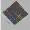 |
Fig. 1. Approximate footprints of the combined MUSE-Deep cubes superimposed on the UVUDF FOV, represented by the PSF matched F275W frame. Colors to help distinguish individual MUSE pointings and mosaics. |
3. Analysis and results
3.1. Strategy overview
Here, we give a quick overview of the search strategy; each step will be described in greater depth below. In a nutshell, our strategy can be formulated: “Detect every source present in a given UV filter, and subsequently use images in additional, redder, filters as well as ancillary information to determine for each source whether it is consistent with being escaping LyC radiation in the detection filter.” To this end, we first ran source finding and detection routines on each of the three background subtracted (Sect. 3.2) UV filter images using a set of settings that ensured that we catch as many faint but real sources at the cost of yielding a potentially substantial number of spurious detections (Sect. 3.3).
Using the segmentation maps created in the source detection step, we extracted fluxes for each segment in each of the eleven filters (or the available subset hereof, Sect. 3.4). For each filter, the adjacent filter to the red side was used as a verification filter; any detection that was not also detected in the verification filter was immediately rejected (Sect. 3.5.1). Since we are searching for objects at a redshift that puts LyC in the detection filter and nonionizing UV continuum in the verification filter, we also required that an object must be of lower mAB in the verification filter than the detection filter (Sect. 3.5.2). Figure 2 shows throughput curves of the three UV filters and, for each of them, its pivot wavelength and the redshift at which the Lyman edge of 912 Å falls approximately at its red edge. Also shown is the optical filter F435W, used for verification of sources detected in F336W (see below).
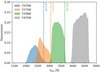 |
Fig. 2. Filter throughput curves for the three detection filter plus F435W. For each detection filter, we also show the approximate lower redshift cut-off for galaxies to be reliably detected in LyC. Verification of detections in any filter is done in the filter immediately to the right. |
We then moved on to visual inspection of the remaining segments for morphology and for their spectral energy distribution (SED), to remove objects that are clearly not LyC leaking galaxies at redshift 1.9–3.5 (Sect. 3.5.3). Next, we matched the remaining objects to the catalogs of R15 and I17 for existing photometric or spectroscopic redshifts. We also performed our own SED fitting using BAGPIPES (Carnall et al. 2018), and extracted spectra from the MUSE-DEEP public datacubes for selected objects. Where present and of medium or high certainty (see Sect. 3.5.4), spectroscopic redshifts were given priority. Where only photometric redshifts were present, we made a case-by-case assessment. Our final list of seven candidate objects is tabulated in Table 1, which lists their sky coordinates as well as the catalog IDs of the corresponding objects in the catalogs of R15 and I17.
Candidate objects coordinates and basic properties.
We finally remeasured fluxes for the remaining candidates in all available filters integrated in a circular aperture with a fixed diameter of  (Sect. 4.1). This aperture size is equal to the value of the seeing adopted in I17, and we found that it encompasses the majority of flux from our remaining candidates, unlike the often small image segments found from source detection in the rest-frame FUV. These fluxes enabled us to find integrated stellar population properties, which, in turn, allows for a more direct comparison to other galaxies in the literature.
3.2. Background subtraction
We modeled and subtracted the backgrounds of all drizzled and PSF matched images using the python photutils package (Bradley et al. 2020), using the Background2D class, which estimates the background locally on a mesh, based on sigma clipping statistics, and subsequently interpolates this background mesh to the resolution of the original image. We used the default SExtractorBackground background estimator and StdBackgroundRMS background RMS estimator.
Following the recommendations from the photutils authors, we estimated the background in two steps. In the first step, the background was estimated and subtracted on the unmasked images. We then ran the make_source_mask function, which uses sigma clipping statistics for an initial noise and background estimate, then uses this to detect sources, create a segmentation map, dilate the source segments, and finally output a mask array. This mask was then passed to a second iteration with the Background2D class, along with the unmodified data frames, from which the resulting background image was finally subtracted.
The UV frames contain quite complex and strong features, what the authors of R15 describe as a “blotchy pattern,” which, given the relatively weak signals and strongly correlated noise patterns, could lead to over- or underestimation of flux in certain regions, in turn bringing detected flux below the signal-to-noise threshold or even below zero, if not properly modeled and subtracted. It was therefore necessary to choose a box_size small enough to encompass the characteristic size of these blotches, in order to model these residual patterns, yet large enough to not include noise in the model.
In the optical/red and IR filters, extended red stellar populations become visible in the field’s elliptical galaxies. These pose a challenge for background subtraction, as they require either large box sizes or strong mask dilation in order to avoid subtracting the outer stellar halos. We opted for a combination of the two, although with the main emphasis on larger box size, since the background in the optical and red filters has less structure than in the UV, and since there are so many objects visible in the red and IR filters that dilating the masks would unnecessarily remove a large fraction of the background pixels, severely impacting the quality of background modeling. We note that due to the fact that we target relatively high surface brightness and compact sources, this will make only a small difference to the final photometry in the redder bands.
In Appendix A, we show examples of background and background subtracted data in F225W and F775W to illustrate the different challenges presented by the UV and red data. Parameters passed to the source mask creation and background modeling routines for each filter were determined by trial and error, visually inspecting the modeled background for over- or undersubtracted regions near masked sources, and artifacts of poorly modeled background. The parameters that we finally settled on are tabulated in Table A.1.
3.3. Source detection and deblending
We first ran the photutils source detection routines detect_sources() with settings that prioritized completeness in detection over avoiding spurious detections, since these, as discussed below, will be rejected in later steps. We then passed the resulting segmentation maps to the function deblend_sources() to deblend overlapping galaxies. In this step, we again allowed the algorithms to deblend too many rather than too few sources, since LyC escape is a local phenomenon that will not suffer any missed detections due to this, while larger apertures, as discussed in Sect. 4.1, may dilute the S/N of a detected source below our threshold value. This resulted in a deblended segmentation map for each of the three UV filters. For each of these, we then extracted fluxes in all segments in every one of the remaining filters, including the two remaining UV filters. Based on S/N and color selection criteria described below, we could then reject objects that are inconsistent with being LyC leakers detected in the ionizing continuum.
Working on PSF-matched data comes at a cost in terms of image depth, since the UV and optical data are convolved and mixed with a number of pixels that contribute only noise, degrading the signal-to-noise ratios of fluxes measured in these images. Rafelski et al. (2015) have opted to optimize their photometric depth by measuring all fluxes in unconvolved data, and subsequently applying an aperture loss correction in the NIR data, where the PSF is significantly larger than in the UV/optical bands. However, such an approach would result in practical difficulties in this work, rendering it unfeasible. Most importantly, such an aperture correction accounts for flux lost outside aperture due to convolution with the PSF, but not for flux from outside sources bleeding into the aperture. When using the NUV bands for detection images, a given segment used for photometry may only cover a small part of a galaxy and in general not the part that is brightest in the optical and NIR bands, and thus flux from neighboring regions may bleed into the segment in bands with larger PSF. Thus, when performing photometry on segments of galaxies, this must be done on PSF matched images.
3.4. Photometry and uncertainties
For each or the three UVUDF filters, we created a segmentation image as described above, and proceeded to measure fluxes in all segments of this image for every one of the filters listed in Table A.1, resulting in a measured flux in 11 filters for each segment in each of the three detection images. We reestimated the errors on the measured fluxes by random sampling of the surrounding background. Because of drizzling and PSF matching, the noise is correlated, so a simple pixel-to-pixel variance estimate is not sufficient. Instead, for each of the labeled segments, we extracted the flux in 200 apertures randomly placed within a square region ±300 pixels surrounding the segment. For simplicity, we created circular apertures each of the same pixel area as the segment. From these 200 segments, we computed the standard deviation of the computed fluxes and adopted this value as the error on the originally measured flux. We performed this procedure for the three UV filters F225W, F275W, and F336W only. The general S/N is much higher in the optical and IR filters, and the field gets crowded there, making the random aperture placement impractical.
3.5. Sorting and selection
3.5.1. By Signal-to-noise
The detection and deblending procedures described above yielded 2187, 2520, and 1804 segments in F225W, F275W, and F336W. One would probably expect more detected objects for longer wavelength filters, but we deliberately set the detection and segmentation limits to allow for spurious detections, of which we expect to find more in the bluer filters where noise levels are higher and throughput lower.
While random fluctuations can align to yield spurious detections, the probability of this happening within the same small area of a few tens of pixels in adjacent filters is small, and such a chance alignment would be caught when examining the full SED. Therefore, our first selection criterion was that a detection in any given segment be > 2σ in both the detection filter and in its red-adjacent filter, such that detections in F225W must be ≥2σ also in F275W, detections in F275W must be ≥2σ also in F336W, and detections in F336W must be ≥2σ also in F435W. The dual-band S/N filtering left 1084, 1183, and 1261 segments in F225W, F275W, and F336W, respectively.
3.5.2. By UV colors
As a next step, we applied as a filtering criterion that the measured magnitude in the detection filter be larger (fainter) than in the adjacent filter to the red side. Typical star-forming galaxies have a UV fλ spectrum defined as a power law with an exponent, the UV slope, of β ∼ −2. This corresponds to a flat spectrum in fν units and a flat SED in AB magnitudes. Both dust and ISM attenuation will affect the bluer filter more strongly than the redder one, and thus, the observed ratio of ionizing-to-nonionizing flux will be a measure of the escape fraction fesc, LyC. No stellar population modeling we know of does predict any populations that intrinsically have higher fν fluxes at restframe ∼800 Å than at restframe ∼1000 Å, as the filters will approximately probe. Even in case they exist, wavelength-dependent attenuation by dust will suppress F800 more strongly than F1100. The only empirically based dust attenuation law that covers the extreme UV wavelength domain (Reddy et al. 2016) is particularly steep in this range and thus, even the modest difference in rest-frame wavelength can mean a significantly stronger attenuation at λrest = 800 Å than at λrest = 1000 Å. In addition, LyC is absorbed when interacting with the neutral ISM, which will suppress the F900/F1500 ratio further. LCEs have been observed with relative (i.e., not accounting for dust attenuation) escape fractions from almost zero (Leitet et al. 2011, 2013; Puschnig et al. 2017) to close to 100% (Rivera-Thorsen et al. 2019). This further suppresses F900/F1500 for a given galaxy.
Finally, at redshifts z ≳ 2, absorption by the neutral fraction of the IGM becomes significant. The average IGM attenuation due to ionization of rest-frame λ ∼ 880 Å photons emitted at redshifts 2 (3) has been modeled by Inoue et al. (2014) to be 0.3 (0.8) mag, corresponding to an average transmission factor of ∼0.76 (∼0.48). These numbers are, however, subject to a large scatter (see, e.g., Vasei et al. 2016, for an example distribution at z = 2.4.).
With these combined attenuation effects on ionizing photons emitted within 2 ≤ z ≤ 3.5 in mind, we require our sources to be fainter in the detection filter than in its red-adjacent filter in order to be a believable LyC source. Applying this criterion left 385 segments in F225W, 598 objects in F275W, and 861 objects in F336W. It is interesting to note that while we detected fewer objects in F336W than the two other filters, more objects are left in this filter after the S/N and color criteria have been applied.
3.5.3. By morphology and visual inspection
After these initial filtering steps, we produced an SED plot as well as a series of “postage stamp” images of all remaining objects. By visual inspection, we removed all segments that were clearly fragments of larger nearby galaxies, as well as a number of edge cased that were difficult to automate. In some cases, a candidate had two nearby matches in the I17 catalog of strongly differing redshifts, and a visual inspection was the best way to determine whether our candidate was associated with one or the other, or the two were too strongly blended to tell apart. Among the galaxies without matches in the I17 catalog, some met the color selection criteria above but the combination of their brightness, morphology and very red SED led us to reject them as nearby interlopers. In other cases, faint detections in the UV that passed the selection criteria, showed so strong blue colors that they were undetected in the optical and IR filters and thus not suitable for further investigation. A few spurious detections had made it this far as well but were easily identified from inspecting their SED and images.
3.5.4. By spectroscopic redshifts
Spectroscopy, where available, is the most reliable way of measuring redshifts. Inami et al. (2017) publish a catalog of 1574 spectroscopic redshifts in the HUDF, of which 1338 are reported as high quality redshifts. We matched our candidate objects with the I17 catalog by searching for sources within a radius of  , slightly above the reported FWHM seeing in Inami et al. (2017), beyond which contamination from nearby compact sources is weak, and listed for each of our sources all MUSE sources within this radius. In order to check for contamination and look for sources not found in the catalog, we retrieved the publicly available MUSE-DEEP science cubes. For each galaxy in the sample remaining from the filtering process in Sect. 3.5, we extracted a spectrum from the muse cubes in the following way:
For each object, we determined whether it was contained in the footprint of each of the MUSE-DEEP cubes. For objects contained in a given cube, we extracted all pixels inside a circular mask of radius  and, for each velocity slice, summed up the flux inside this aperture. Objects found inside the footprints of multiple cubes were median-stacked. We then inspected the spectra for line emission; if multiple lines were present, their wavelength separation revealed which lines we were looking at. If only one line was present, we preliminarily assumed it to be Lyα. Spectroscopic redshifts found by this procedure are, where available, tabulated for objects of interest in Table 2.
Photometric and spectroscopic candidate redshifts.
Spectra of Lyman a and surroundings for candidates with Lyman a emission are shown in Fig. 3. Since our extraction was less sophisticated than that of Inami et al. (2017), the resulting spectra are not of the same quality as in I17. Indeed, in a number of cases, where those authors’ redshift determination depends on absorption features, we did not have sufficient S/N to discern individual absorption features. In such cases, we have listed the reported values and compared them to available photometric redshifts and, where not consistently contradicted by these, we have adopted the redshifts of MUSE-DEEP for the given object.
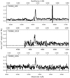 |
Fig. 3. Spectral regions around rest-frame Lyα of the subset of candidate objects with Lyα in emission. At the bottom is shown the observed wavelength scale, above each panel is the corresponding rest-frame wavelength range. |
3.5.5. By photometric redshifts
Included in the catalog of Rafelski et al. (2015) are photometric redshifts computed in two different ways, the Bayesian photometric redshift (BPZ, Benítez 2000; Benítez et al. 2004; Coe et al. 2006), and the redshift as computed by the software package EAZY (Brammer et al. 2008). In addition, in this work, we computed photometric redshifts for the subset of our detected objects that made it through the elimination process in Sect. 3.5, using the stellar population modeling package BAGPIPES (Carnall et al. 2018)2, and the photometric fluxes of the full set of 11 filters where available. We assumed a single population with a delayed τ model, defined as: SFR(t) = t × e−t/τ, where τ is the timescale of exponential decay of star formation. This model provides a good balance between flexibility and simplicity, with an exponential drop-off that allows a span from the strongly bursty to much more extended SFHs. Of the dust attenuation laws implemented in BAGPIPES, we assumed the Calzetti et al. (2000) law, extrapolated to the FUV by a power law (Carnall et al. 2018), allowing AV to vary between 0 and 4 mag, and allowed the redshift to vary freely between 0 and 10. We enabled BAGPIPES’ built-in support for CLOUDY (Ferland et al. 2017) assuming log U = −3 and otherwise using the default settings; this would allow BAGPIPES to also correctly model strong emission line galaxies. BAGPIPES assumes pure Case B recombination and thus zero ionizing escape from the model galaxy (Carnall et al. 2018, Sect. 3).
For IGM absorption, BAGPIPES adopts the analytical version of the IGM transmission law for T(λ, zobs) by Inoue et al. (2014), assuming that all flux with λ < 912 Å is absorbed (this is however already the case when nebular emission is enabled, see Carnall et al. 2018, Sect. 3). We keep in mind that the assumption of zero transmission of IGM could lead BAGPIPES to interpret all data points with nonzero flux as being nonionizing and thus be skewed toward lower-redshift solutions. Mostly, the UV filters have low S/N compared to the optical and IR filters, but if the optical/IR data are more or less evenly consistent with two different models, the presence of nonzero UV fluxes may tip it in favor of the lower-redshift solution.
We then compared the photometric redshifts to those published by Rafelski et al. (2015), as well as the MUSE spectroscopic redshifts published by Inami et al. (2017). Where spectroscopic redshifts exist, we relied on those. Due to the assumption hard coded into BAGPIPES that no ionizing flux reaches the telescope, the minimization algorithm will, if allowed, attempt to adjust the redshift to interpret all bands with measured flux to fall below the Lyman edge at λrest = 912 Å. However, the UV bands have considerably poorer S/N and are less numerous than the optical bands, which counteracts this effect. A discussion of individual objects is given in Sect. 5.2.
3.5.6. Test of redshift with emission lines
For the galaxies in the final candidate selection that show Lyman-α emission, we have measured the equivalent width by measuring the continuum-subtracted line flux in the MUSE spectra, and dividing it by the flux density as measured in an aperture of the same size in the HST filter containing λobs, Lyα. The continuum in MUSE is noisy, and an unknown fraction of it consists of scattered light from the atmosphere, so we preferred the deeper, less contaminated continuum levels from HST imaging. In the case of F336W-1013, Lyα falls between F435W and F606W, and we have used a simple average of the fluxes in those filters to compute the equivalent width. The resulting observed-frame EWs are tabulated in Table 4 along with a number of physical parameters derived from a second round of SED modeling using BAGPIPES (elaborated in Sect. 4.1).
The computed equivalent widths are useful to check for misclassified spectral emission lines. The observed-frame EWs range from 118 to 210 Å, which in the restframe yield ∼30–50 Å. Other comparably strong emission lines are found from rest-frame [O II]λλ 3727,3929 Å and redward, where the redshift corrections to the measured EWs are lower by roughly a factor of three or more. This leaves only few lines that could be consistent with the measured values. For example, [O II] λλ 3726,3729, could possibly be consistent with the measured lines, but this feature is a multiplet; and at such redshifts, lines such as Hβ, the [O III] doublet at λλ 4960,5008 Å, and Hα would all fall within the redshift range of the spectrograph, none of which are found. We also note the dual asymmetric peaks shape of the line in F336W-189, a typical and unique feature of Lyα; and the clear asymmetric shape of F336W-1041, typical of a Lyα line at modest S/N.
3.5.7. Final selection
The previous steps in combination left us with a selection of seven objects of interest, listed with their R15 and I17 counterparts where available in Table 1. The strongest candidates shown in bold type in Table 1 and subsequent tables. These all have spectroscopic redshifts in I17 at reported confidence levels 2 (F336W-1013, F336W-1041) or 3 (F336W-189, F336W-554), and we were able to confirm the spectroscopic redshifts from our own extracted spectra. In addition, these candidates all have flux measured at at least 2σ in at least two filters that are entirely in the rest-frame LyC at the spectroscopic redshift, except for (F336W-1013).
In addition, we have identified three second-tier candidate objects that we consider highly likely, but not definitive, leakers. Two of them have no spectroscopic redshift, but the available photometric redshifts are high enough that the flux in the FUV filters must be dominated by LyC; and one has a convincing spectroscopic redshift that is however only marginally consistent with being a LyC leaker. A discussion of these is given in Sect. 5.2.
Figure 4 shows 1.7″ square cut-outs in the filters from F225W to F775W, as well as an RGB composite of the filters F775W, F606W, and F435W in the R, G, and B channels, respectively.
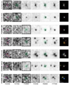 |
Fig. 4. Postage stamp images in the filters F225W-F775W of the candidate objects, as well as a composite image of F435W, F606W and F775W for each candidate. The detection segment and the larger photometric aperture are shown in green in F606W as well as in the detection filter for each candidate. The reddest LyC-dominated filter is framed in thick black dashes for each candidate, and contours of the brightness in F775W are shown in F225W to provide a morphological comparison between the rest-frame far- and near-UV bands. The cut-outs are 2.7″ on a side. |
4. Candidate characterization
4.1. Fixed-aperture photometry and global SED modeling
Up to this point, all fluxes have been measured in the segments created from the source detection in the UV filters. The young stellar populations that dominate production of UV photons are generally significantly more compact than the older populations that often dominate the optical and IR bands. Our choice of aperture thus yields comparatively high fluxes in the UV filters compared to what would result from photometry of the entire galaxy.
To derive global physical properties for the candidate galaxies rather than local properties for the often small regions defined by the segmentation maps, we have supplemented these measurements with fixed-aperture photometry for the objects we found to be LyC leaker candidates. We chose a fixed circular aperture  in diameter, which is large enough to encompass the majority of most galaxies in the relevant redshift range, and small enough to keep the risk of contamination from nearby objects low. In Fig. 5, we show the resulting SEDs for the candidate objects listed in Table 2, this time shown in AB magnitudes. The same magnitudes are tabulated in Table 3. Figure 6 shows the SEDs for segment and fixed-aperture fluxes in fλ units, along with the best-fit spectra based on the segment fluxes. We note that that this larger aperture made the MC sampling of uncertainties unfeasible. With aperture size grows also the probability of catching a bright nearby object in the aperture which will skew the standard deviation. For this reason, we have found this method unfeasible with a
  aperture, and have opted to simply report the uncertainties found from the RMS frames. Additionally, the compactness in the UV bands has the consequence that a larger number of pixels will contribute. As a result, the errors reported from fixed apertures are markedly larger than from segmentation images, with some measurements being consistent with 0 within 1σ. We have opted to report these as measurements with error bars rather than upper limits in Table 3 and Figs. 5 and 6, but have not based any quantitative conclusions on these.
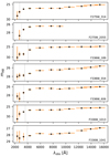 |
Fig. 5. Spectral energy distributions of the leaker candidates, extracted in circular apertures of radius |

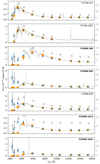 |
Fig. 6. Segment fluxes (blue) and fixed-aperture fluxes (empty circles with the flux scale on the right) shown with BAGPIPES posterior photometry (orange dots) and model spectra (gray shading). |
Segment-measured AB magnitudes for the candidate objects in the five bluest filters in the UVUDF.
After completing the redshift and color selection process, we revisited the BAGPIPES SED fitting for the remaining candidate objects, this time based on fluxes extracted from the fixed-size apertures. This time, we fixed the redshifts at the spectroscopic values where available, and in the two cases where this was not the case, we left it open as a free parameter. Again, we assumed a delayed τ model, finding it to be the one single model which can cover the widest range of physical properties, but this time we imposed a metallicity constraint of Z ≤ Z⊙. In Table 4, we tabulate the best-fit values of core properties obtained from this second run.
Best fit physical properties of leaker candidates.
4.2. Ionizing escape fractions
Following Steidel et al. (2001), Siana et al. (2007, 2010), Grazian et al. (2016), and Fletcher et al. (2019), we define the relative and absolute escape fraction in the following way:
where (f1500/f900)Int and (f1500/f900)Obs are the intrinsic and observed ratios of flux density at rest-frame wavelengths 1500 and 900 Å, TIGM is the IGM transmission coefficient along a given line of sight, and A1500 is the attenuation at rest-frame wavelength 1500 Å in magnitudes. Often, an intrinsic flux ratio of (f1500/f900)Int = 3 (in fν units) is assumed (e.g., Steidel et al. 2001; Grazian et al. 2016, 2017); however, the value has been found to vary from 1.7 at a burst age of 1 Myr, to 7.1 at 0.2 Gyr of age, using the stellar population library of (Bruzual & Charlot 2003; Grazian et al. 2016), and where possible, it is preferable to estimate the intrinsic ratio for each individual galaxy.
In this work, we have opted to find  directly from the BAGPIPES models, and then applying the dust correction described above to find
  , and then apply a corrective term to account for IGM absorption as described in the next section.
We have estimated the absolute ionizing escape fraction by comparing observed LyC fluxes to modeled intrinsic fluxes in the following way: For each best-fit BAGPIPES model, we constructed a model galaxy based on the fit, but omitting the effects of internal dust, ISM, and IGM absorption. We then compared the observed LyC fluxes in the reference LyC filters shown in Fig. 4. The fraction of model-to-observed flux is the combined transmission galaxy ISM and the IGM. We then estimated the relative escape fraction of each candidate, by applying the best-fit dust attenuation at rest-frame 1500 to the absolute fraction.
Figure 7 shows for each candidate the observed fluxes (blue, filled circles), along with the best-fit, IGM-attenuated spectrum (strong orange) and the dust- and ISM-free, but still IGM-attenuated, model spectrum (black). Each of these is additionally shown with the BAGPIPES-generated IGM attenuation removed, shown in a lighter tone (pale orange, gray). Synthetic HST filter photometry, also generated by BAGPIPES, is shown as open circles in the colors of the corresponding model spectrum. The absolute escape fraction can then be visually understood as the fraction of the values marked by the filled blue to the open gray circle in the reference LyC filter. It is worth noting that while a similar interpretation of the relative escape fraction as a ratio of the filled blue to open light orange circles would be physically correct, it is not the value found as  using the convention described in Eq. (2). That convention assumes the dust attenuation to be the same at 900 and 1500 Å and thus yields a lower fraction than what would be found by directly measuring the ratio of escaping to dust-corrected intrinsic flux at 900 Å; the discrepancy between the two will depend on the choice of dust attenuation law.
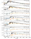 |
Fig. 7. Dust-, ISM-, and IGM-corrected model spectra of the candidates, as well as observed (filled circles) and model predicted (open circles). Orange spectra are the BAGPIPES best fit to the observed data points. Model spectra generated from the same best-fit parameters, but with ISM and dust removed, are shown in black. Gray spectra show the ISM- and dust-free model spectra corrected for the BAGPIPES assigned average redshift-dependent IGM absorption. |
It is interesting to note from inspection of Fig. 7 that while the relative escape fractions can be even quite dramatically higher than 100%, all absolute escape fractions seem roughly consistent with being ≲1, even for an object like F336W-1013, for which the relative escape fraction is ∼450% (see Table 5) after IGM correction. The relative escape fraction is computed based on the assumption that the light from the stars responsible for emitting LyC undergo the same dust attenuation as the full stellar population, on which the galaxy model is built. However, recent studies of the Magellanic clouds (Ramachandran et al. 2018b, 2019; Doran et al. 2013) have shown that the ionizing output from a galaxy can be completely dominated by as little as one to a few dozen extremely luminous, massive stars. If these stars are seen along a privileged line of sight through the dust in their galaxy, they could conceivably be much less attenuated than the greater stellar population. This could be due either to a highly clumpy dust geometry or to the stars dominating LyC emission being located away from the stars emitting the bulk of rest-frame 1500 Å photons (see e.g., Ramachandran et al. 2021, for an example of O stars residing in the tidal bridge between the Magellanic Clouds).
Escape fractions and IGM correction.
One candidate, F336W-1041, has an absolute escape fraction of ∼100% even before IGM correction and thus requires an essentially completely dust- and gas free line of sight between the emitting stars and the telescope for the observed escape fraction to be physical, and other candidates require similar, intrinsically quite unlikely, constraints on intervening dust and H I column to be fulfilled. However, it should be kept in mind that we have introduced a strong selection bias favoring exactly such conditions.
4.3. IGM correction
BAGPIPES accounts for IGM attenuation following Inoue et al. (2014), applying an average redshift-dependent IGM attenuation curves derived in that paper (Carnall et al. 2018). While this can be useful to generate a realistic, generic model galaxy at a given redshift, IGM absorption along a given line of sight is highly stochastic, as shown for example in Vanzella et al. (2015), Vasei et al. (2016), Bassett et al. (2021), or Bassett et al. (2022). Specifically, Jones et al. (2021, Fig. 6) show that the average IGM optical depth to LyC changes drastically over the range of wavelengths of this work. In addition, as discussed above, in this work, we are selecting specifically for high-transmission lines of sight, and thus an unbiased average is unlikely to be a good approximation to lines of sight actually observed.
To obtain a realistic estimate of the impact of IGM absorption on the observed LyC fluxes, we first ran Monte Carlo simulations of 1000 random, unbiased lines of sight following the prescription given by Inoue et al. (2014). We next imposed as a prior constraint on these lines of sight that they must be consistent with an  . All lines of sight not meeting this requirement were removed from the LOS distribution. Next,
  was found assuming the IGM opacity of each line of sight, and a resulting distribution of escape fractions was found. For each candidate, we then report the mean and standard deviation of this distribution as the escape fraction. One galaxy, F336W-1041, has
  , requiring an IGM transmission of unity, to which we have fixed it.
In Table 5, we report the measured and absolute escape fractions without IGM correction, as well as the derived mean and standard deviation of the IGM transmission coefficient TIGM and the resulting IGM-corrected absolute escape fractions. Uncertainties quoted for the latter are based solely on the IGM distribution; the galaxy models and measured LyC fluxes are assumed as is, without uncertainties. The uncertainties on the model galaxies are dominated by systematics due to the choice of star formation history, dust attenuation law etc., and the uncertainties on the IGM transmission and the measured LyC fluxes are highly degenerate. A stricter treatment of uncertainties of the escape fractions would entail a full MC sampling of the LyC fluxes for a variety of SF histories and dust attenuation models, as well as creating a full TIGM distribution for each realization, which is outside the scope of this work.
4.4. Contribution to ionizing background
We have estimated the contribution from our candidate objects to the metagalactic ionizing background at redshifts 2 < z < 3.5 broadly following the methodology of Jones et al. (2021, Sect. 6). We have converted the measured flux densities to an ionizing emissivity at 900 Å ϵ900, defined as the luminosity density at 900 Å per unit frequency per unit comoving volume.
For each of the candidates, we have used the flux density in the reference LyC filter shown in Fig. 4, and assumed the measured filter average as the value at 900 Å. This conversion assumes that the measured flux in this filter is a good representation of the spectral flux density at rest-frame 900 Å or, equivalently, that the spectral shape of the LyC in the wavelength ranges covered by these filters is constant in fν units. Looking at the fluxes in Fig. 6, the measured differences between the reddest and neighboring bluer filter are nowhere more than × ∼ 1.5, making this an imperfect but reasonable assumption.
We computed an ionizing luminosity density from each measured flux density by correcting it for IGM absorption using the values derived in the previous section, and multiplying the result by  , where DL is the luminosity distance at the given redshift. We then computed the comoving volume defined by the dA = 160″ angular size of the UVUDF and the redshift range defined by our filters, 2 < z < 3.5, as:
where Ac(z) is the comoving area defined by the angular size dA of the field at redshift z, and drc(z)/dz is the thickness of the slab defined by the redshift difference dz at redshift z. We have assumed that measured LyC emission is isotropic which is not generally a good approximation for single galaxies, but which from symmetry considerations should be a reasonable assumption for the number of sources existing in the HUDF within our redshift range. We have found found a resulting value of 
 erg s−1 Hz−1 cMpc−3 for the full (tier one only) set of candidates.
This value is shown in Fig. 8 along with predictions and measurements from the literature. We find that our values are consistent with those found by Jones et al. (2021). Once corrected for IGM attenuation, the resulting emissivity from star-forming galaxies is sufficient to maintain the measured ionization state of the Universe up to redshift ∼3.5. The value we find for ϵ900 is rather high, but still consistent with, values previously found for example by Jones et al. (2021), and is dominated by one galaxy, F336W-189, which contributes 83% of the total, IGM-corrected ionizing luminosity, owing at least in part to a strong IGM correction. With its high redshift and low value of  , it allows for low-transmission IGM lines of sight and thus drives the median IGM correction up.
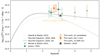 |
Fig. 8. Ionizing volume emissivity derived from the galaxies of this work compared to other measurements and predictions in the literature. Gray dashed and dotted lines show the theoretical models for bright AGN by Faucher-Giguère (2020) and Haardt & Madau (2012), and the fully drawn line shows the combined model of AGN and star formation from Faucher-Giguère (2020). Light green plus signs show the ionizing field in various redshift bins measured from the IGM properties by Becker & Bolton (2013). Dark green diamonds show the emissivity from star formation measured by Jones et al. (2021), and the single dark cross shows the estimate from Steidel et al. (2018). The filled orange marker shows the value derived from only the four tier one candidates in this work, while the open orange marker shows the value derived assuming that all the candidates are bona fide leakers. The open yellow marker shows the same as the open orange marker, but not corrected for IGM absorption. The orange and yellow markers are showed a bit offset on the redshift axis for visibility, but all are measured in one single redshift bin of 2 < z < 3.5 (illustrated with the horizontal yellow bar), with an average redshift of 2.81. |
We estimated the effect of cosmic variance on our results using the QUICKCV cosmic variance calculator (Newman & Moster 2014; Moster et al. 2011) and, independently the Trenti & Stiavelli online cosmic variance calculator3 (Trenti & Stiavelli 2008). Both yielded an estimated cosmic variance of ∼15–20% on the emissivity, significantly less important than the uncertainties stemming from photometry and the inherent stochasticity of the IGM.
5. Discussion
Resulting from our selection and inspection criteria, we have compiled a set of candidate LyC leaker galaxies falling into two tiers as described in Sect. 3.5.7. Based on best-fit models of their stellar populations, we have derived intrinsic and dust-attenuated LyC outputs and, based on these as well as Monte Carlo simulations of the IGM, derived the absolute and relative LyC escape fraction of each candidate galaxy. We have found that while some galaxies have surprisingly strong LyC fluxes, they are all roughly consistent with an absolute escape fraction of ≲100%. However, some of the candidates show relative escape fractions of several hundred percent, something that requires the LyC emitting stars to be seen through a considerably lower dust column than the general stellar population dominating the optical and IR filters. We discuss these cases below.
We then used the resulting IGM absorption distributions to convert the observed LyC flux densities to a cosmic volume emissivity ϵ900, and compared it to theoretical and observed values in the literature. We find a value that is surprisingly high, but consistent with measured values from the literature (Becker & Bolton 2013; Jones et al. 2021). The emissivity is dominated by one galaxy, F336W-189, which contributes 82% of the combined volume emissivity, with F336W-1013 contributing an additional 10%. Both galaxies have high redshifts and as a result, a TIGM -distribution skewed toward low transmission and thus a strong ISM correction. Despite the fact that as many as four of our candidate galaxies are unlikely to have been found in any typical preselection methods, it is thus not immediately clear how important their contribution to the cosmic ionizing background is, mainly due to the statistical uncertainty in the IGM corrections.
5.1. Strongest candidates
F336W-189. This galaxy was also identified by Saxena et al. (2022), and is our strongest candidate. It is bright, has a strong and unmistakable Lyman-α emission line (see Fig. 3) that determines its redshift beyond any reasonable doubt, and the MUSE and Photutils centroids are coincident to within  . It is detected in three bands in LyC, and its SED is textbook example of what we would expect a star-forming galaxy with a modest
  to look like. It was detected in F275W but rejected because it is fainter in F336W than F275W, because both filters are in the rest-frame LyC. We find a stellar mass of log(M*) = 9.58 ± 0.02, the most massive of the candidates. The absolute escape fraction is 36% ± 22% and, after dust correction, we find a relative escape fraction of 325%. The Lyα line profile is double-peaked with a peak separation of Δv ≈ 620 km s−1. Verhamme et al. (2015) found that a peak separation of Δv ≲ 300 km s−1 corresponds approximately to log NH I ≈ 17, at which point τ900 Å ≈ 1, meaning that
  (LyC) for this galaxy is a good deal higher than expected from the peak separation (but as discussed above, the clumpy nature of dust may have inflated the relative escape fraction substantially and makes a comparison to theoretical values tricky). This galaxy also dominates the found value of ϵ900, contributing 83% of the total IGM-corrected ionizing flux in the searched volume. This large contribution owes at least in part to the low measured, IGM-uncorrected escape fraction, which is consistent with IGM lines of sight
F336W-554. This galaxy does not show any line emission, emission in Lyα, but its spectroscopic redshift of 2.87 from I17 is reported with a confidence level of 3, the highest in that work, based on multiple absorption features. The two photometric redshifts from R15 are both slightly higher, at 2.97 and 2.97, also reported at a high confidence level. The morphology of this source seems point-like, or at least very compact, in F336W. It is situated at the northern tip of a more extended feature seen only in the nonionizing filters. Another object is seen nearby to the NW (upper right) in all filters. This object has ID #6770 in R15, where it has zphot ≈ 1.55 with both their methods, but has no counterpart in I17. The two galaxies are well separated visually, but at a projected physical distance of ∼5 kpc at z = 1.55, it is in principle possible that a source associated with this object could contaminate our source, but given the more obvious association with the source to the south with secure spectroscopic redshift, we believe it represents genuine LyC emission. The fluxes measured in the rest-frame LyC for this object are very high. It is quite young and with log(M*)≈8.8 in the lower mass end of our candidate list. It does however contain quite a lot of dust, which seems difficult to reconcile with such strong LyC emission. Indeed, while the absolute escape fraction is 67%, the relative escape fraction is measured to 441%. While this is one of the highest of the derived relative escape fractions, as many as four galaxies have  . This is possible if the LyC emitting stars are seen through a dust column that is considerably lower than that of the stellar population dominating in the optical and IR filters and thus the stellar population models. It is well known that dust can be highly unevenly distributed in starburst galaxies (see, e.g., Menacho et al. 2021, Fig. 4 for an example). Additionally, it has been shown that the LyC output of a galaxy often is dominated by a few, perhaps as little as one or two, bright O or WR stars (Ramachandran et al. 2018a,b, 2019; Doran et al. 2013). These stars can in some circumstances form in the outskirts of galaxies, for example as is the case of the Magellanic Bridge, which contains at least three bright O stars (Ramachandran et al. 2021). The LyC detected in F336W-554 does indeed originate in the outskirts of the galaxy, in a region that is quite faint in the optical and IR bands.
F336W-1013. This galaxy has a spectroscopic redshift from I17 of 2.98, which we have confirmed based on a Lyman α line emission at ∼4840 Å. The photometric redshift methods consistently converge on a redshift ∼2, which could be due to the assumption of a zero ionizing escape built-in to BAGPIPES. The galaxy was detected using F336W as detection filter. It has significant ionizing flux in F275W, and was also found in the source detection step, but fell for the color criterion and was rejected. The galaxy has an ionizing escape fraction of a moderate 15 ± 10% which, in combination with its redshift, leads to a strong IGM correction of the ionizing flux, making this galaxy the second strongest contributor to the ionizing volume emissivity ϵ900, delivering 10% of the total amount of photons. The relative escape fraction of  is another example of a galaxy where the relative escape fraction indicates that the ionizing emission predominantly reaches us through lines of sight that are not typical for the general stellar population. Looking at the F275W cut-out of this galaxy in Fig. 4, there is a brighter area to the W of the central object that, like the artifact next to F336W-1041, is not present in the non-PSF-matched archival frames or the optical or IR frames. We performed the same tests as for F336W-1041 (see Sect. 5.5), measuring signal and noise in the non-PSF-matched data, to check whether the main object, F336W-1013, could be a similar artifact, but found that it persisted at a very similar signal-to-noise as in the PSF matched data. The actual object is actually fainter than this possibly spurious, feature, meaning that at first glance it could easily be discarded as spurious, were it not for its complete spatial coincidence with the feature found in the nonionizing bands. We thus believe it to be real, but the nature of the neighboring feature is still an open question. There is a hint of the same feature, with the same shape, in F336W, but not in any other band. However, none of these concerns are strong, and the Lyα emission line has been identified with strong certainty, for which reason we have placed this galaxy among our most convincing candidates.
F336W-1041. This galaxy consistently converges on a photometric redshift of ∼2.0–2.2 both in our computations and in R15, but has a bright Lyα emission line at redshift z = 3.33 (see Fig. 3), which is also its designated redshift in I17, with a reported confidence level of 2; we speculate that as in the case of F336W-1013, the built-in assumption of zero ionizing escape in BAGPIPES might have skewed its solution toward a lower redshift. There are no strong emission lines consistent with the location of the one observed that correspond to redshifts between 2.0 and 2.2. The high observed equivalent width of the emission feature limits which other lines it could conceivably be, as does the clearly asymmetrical line profile.
F336W-1041 has a relative escape fraction of 397% and an absolute escape fraction of just over, but consistent with, 100%. This means that not only must the line of sight to the LyC sources be completely free of internal stars and dust in the galaxy; also the LOS through the IGM must be essentially free of neutral Hydrogen. This is clearly a priori a very unlikely situation; however, as discussed above, our entire selection process is strongly favoring such a scenario among thousands of originally detected sources, and as argued above, the scenario is not implausible.
The thumbnails in Fig. 4 show that there is a nearby object to the NE of the galaxy. This companion has almost identical redshift in I17 (see Table 2), which we interpret as the two being an interacting pair, and which means that any cross contamination between the two stems from effectively the same redshift and thus will not give rise to false detection in LyC. The flux is surprisingly strong in the LyC, leading us to wonder whether we could be looking at a foreground interloper, but both UV, optical/IR imaging and Lyα emission centroid coincide within a small distance, and the only other visible object in the vicinity has a spectroscopic redshift that would put its rest-frame LyC emission within the same filter as this object. The possibility of a near-perfect alignment with a faint foreground interloper exists, but is statistically very unlikely (Siana et al. 2010; Nestor et al. 2013).
5.2. Other candidates
As discussed in Sect. 3.5.7, our tier-two candidates are what we consider likely, but not definite, candidates. Two of them have convincing and consistent photometric redshifts that correspond to a rather strong LyC emission, but lack spectroscopic redshift. One has a spectroscopic redshift, but in one UV filter, it has S/N < 2, and the next straddles the Lyman break such that the LyC detection there becomes model dependent. The last object has a spectroscopic redshift of 2.98, at which LyC is detected by a solid margin, but the three photometric redshifts are consistently ∼2, which we find calls for caution.
F275W-314. This is the lowest-redshift and perhaps also the least convincing object in the selection. However, it does have a solid spectroscopic redshift, a > 1σ detection in the rest-frame LyC filter F225W, and a flux in the Lyman edge straddling the filter F275W, which is difficult to reconcile with the inferred stellar population. However, this galaxy requires deeper imaging in F225W or a similar filter to be properly convincing.
F275W-2055. This galaxy is not included in I17, and we found no strong emission lines or convincing absorption lines in the MUSE spectrum. Our initial BAGPIPES run yielded z = 2.07 ± 0.08, while the two methods of R15 yielded z = 2.43 and z = 2.26, respectively. However, in our initial SED modeling, we allowed metallicity to vary freely, which yielded an unbelievably high metallicity for this galaxy of Z ≳ 2 × Z⊙.
In our second round of SED fitting, we constrained the metallicity to be equal to or below solar, which bumped up the inferred redshift to z = 2.33 ± 0.29, better in line with the measurements of R15. A redshift of z = 2.38 is where < 1% of the integrated flux in the filter (for a flat spectrum in fλ units) falls redward of the Lyman edge, but the observed flux in F336W for this galaxy becomes difficult to account for without invoking LyC escape already at redshifts z ≳ 2.2, as can be seen in Fig. 6. Even at the original z = 2.07, the measured flux in F275W is inconsistent with the best-fit model if we assume no LyC escape within ∼2σ. An even lower redshift, or a significantly bluer UV spectrum, could bring the measured SED within consistency with an absence of ionizing escape. We note again that the redshift is also downward biased in the fitting process by the built-in assumption of no ionizing escape. When the UV filters have lower statistical weight due to the larger aperture size and the metallicity is constrained to subsolar values, the fit settles on a redshift entirely consistent with those from R15. In this redshift range, the segment based flux in this galaxy is inconsistent with an fesc of zero. The large-aperture F275W flux in this galaxy has a very large error bar, but as mentioned above, two effects inflate this artificially. One is the aperture size itself, which includes more noise to the same signal; the other is that the noise is generally overestimated. We can get a rough estimate of the latter by looking at Fig. C.1, middle panel. Here, the green point cloud shows the ratio of RMS-based to MC-derived errors in the segments, plotted against the measured flux in the segments. The F275W-segment of F275W-2055 has a flux of roughly 0.8 × 10²⁰ ergs s cm2 Å−1, meaning that the error on the flux was over estimated by a factor of ∼3. We find this object convincing, but have assigned it tier two due solely to the lack of a spectroscopic redshift.
F336W-606. The second of two candidates that have no spectroscopic redshift. For this galaxy, the R15 photometric redshifts are 2.50 and 2.69. Our original BAGPIPES redshift is 2.41 which however shifts to z = 2.73 when the metallicity is constrained as described above. The galaxy has S/N > 2 in all three UV filters, but only picked up by our detection and filtering procedure when using F336W as detection filter. In F225W, it falls for the color criterion. It is unclear what is the reason why it is rejected when using F275W, but given the faintness of the source, it is conceivable that the structured noise could have been included in the image segment, and the difference in segment shape could dilute the S/N below the 2σ threshold. Morphologically, this is a complex object that consists of one major, bright, compact feature to the SW, and a collection of multiple fainter clumps to the NE (see Fig. 4). These features are all treated as one feature in R15, while we have based our SED modeling on a small segment of the NE feature collection, and even in the  aperture, the two parts are separate. The combination of strong flux and consistent photometric redshifts make this an interesting candidate object, but the lack of a spectroscopic redshift is is a concern.
5.3. Other LyC surveys in overlapping fields
5.3.1. Jones et al. (2021)
Jones et al. (2021) carry out a search for LyC leakers in the GOODS fields using the publicly available F275W observations from the HDUV survey and archival spectroscopic catalogs to select galaxies in the redshift range 2.35 < z < 3.05, in which the HST F275W filter probes only the LyC, while the adjacent F336W at least partially probes the nonionizing UV continuum. Given coordinates and redshifts from the HDUV catalogs, they then lay down a 2″ circular aperture on the given locations in F225W, and measure the flux in search of significant LyC detection, and then go through various steps to control for contamination from interloping galaxies. They find three candidate objects in GOODS-S, of which one, a galaxy at z = 2.678 is contained in the UVUDF footprint. We found this object during source detection in F275W, but it was subsequently discarded because the segment had a signal-to-noise in F336W of only 1.7 (S/N criterion), and is 0.9 mag fainter (color criterion). We have thus not reached the point of extracting MUSE spectra or performing SED fitting for this object. We note that our method uses small apertures, which only encompass the bright region in the detection image, and relatively aggressively splits any clumpy source up in multiple segments. This means that our method is quite robust to contamination from nearby objects, while it is vulnerable toward configurations where the ionizing radiation may emanate from regions that are faint in nonionizing UV continuum. Jones et al. (2021) use a larger aperture, encompassing the entire galaxy and catching all flux within a radius of 1″, making this method more robust to scenarios where there is an angular offset between ionizing and nonionizing UV radiation, but more vulnerable toward inaccuracies in background subtraction, contamination from adjacent objects, etc. Jones et al. (2021) do not find our object F336W-554; It is unclear why, as these authors have used the catalogs of I17 for preselection of candidates, and the object is found within the redshift ranges that they probe.
5.3.2. Saxena et al. (2022)
Saxena et al. (2022) search for LyC leakers in the CDF-S, a superset of the HUDF. In their work, they look at galaxies at 3.1 < z < 3.4 preselected from photometry or MUSE-DEEP, find spectroscopic redshifts in the VANDELS catalogs (McLure et al. 2018), and look for LyC emission in archival photometric data. They find 11 LyC leaker candidates in the greater field, of which four are contained in the HUDF, including the one we label F336W-189 and these authors label CDFS-12448. Interestingly, this object is the only overlap between our candidates and those of Saxena et al. (2022): Our method did not yield any of their other three objects inside the footprint of the UVUDF: CDFS-13385, CDFS-15718, or CDFS-16444.
CDFS 12448. As discussed above, this is the same object that we denote F336W-189, and we agree that it is a strong LyC leaker candidate.
CDFS 13385. We detected this galaxy in all the three detection passes. In F225W and F275W, it fell for the color criterion discussed in Sect. 3.5.2, meaning that the detection filter was brighter in AB magnitudes than the next redward filter. When detected using F336W, it passed these criteria and was selected for SED fitting. Our SED fitting yielded a photometric redshift of  . We compared this to Rafelski et al. (2015) who reported the redshifts z = 0.09 and z = 0.20 with their two independent methods. In Inami et al. (2017), the object’s redshift is reported with a confidence level of 2 out of 3, or “fairly strong,” based on identification of Lyman-α in emission. However, given the SED and the agreement between the three photometric redshifts, we find it likely that the redshift in Inami et al. (2017) is based on a misclassified [O II] λλ 3727,3729 doublet, which at a redshift of ∼0.44 would fall at the wavelength of Lyman α at the redshift reported by Inami et al.. At this redshift, the doublet would have a peak separation of ∼4 Å, corresponding to a peak separation of ∼225 km s−1, which could reasonably be mistaken for a z = 3.4 Lyα profile by an automated survey.
CDFS 15718. This galaxy is not detected in the HST UV filters in the UVUDF, despite these observations being quite deep. At its redshift of z ≈ 3.44, the Lyman edge falls around 4050 Å, close to the red edge of the NB396 narrow band filter at the 2.2M telescope at La Silla, in which they have observed the reported LyC emission. F336W, on the other hand, falls blueward of NB396, between ∼3100 and ∼3700 Å. It is possible that a Lyman Limit system exists between the galaxy’s redshift of 3.44 and z ∼ 3.05, where LyC would enter the red side of F336W. This could conceivably allow a window of LyC to reach Earth and be be detected in NB396 but not F336W.
CDFS 16444. We have not detected this galaxy in F336W either. As with CDFS 15718, Saxena et al. (2022) report this galaxy detected in LyC in the NB396 filter. This galaxy is located at z = 3.13, leaving the window of 3.05 < z < 3.14 for a possible Lyman Limit system to absorb escaping LyC on its blue side.
Conversely, the method of Saxena et al. did not yield either of the objects labeled F336W-1041 or F336W-554 in this work. The latter is easily explained, as its spectroscopic redshift is outside their redshift range of interest. F336W-1041, on the other hand, is within the redshift range, but not listed among their candidates.
5.3.3. Redshift distribution
Of the three redshift bins defined by the wavelengths of the detection filters, our leaker candidates were found predominantly in the highest redshift bin, with no candidates found in the lowest redshift bin. The latter can be at least partially explained by the large overlap in transmission of F225W and F275W; the volume unique to F225W is small, and F275W is deeper. If the Lyman edge of a galaxy falls within F225W, the distinction between ionizing and nonionizing radiation becomes difficult and model dependent. If on the other hand it falls entirely redward of this filter, only a narrow redshift window exists before it also drops out of F275W.
It is somewhat surprising that we find the leaking candidates so predominantly at higher redshift, given that the IGM becomes more opaque at the higher redshifts. The comoving volumes probed by the two highest-redshift filters are the same order of magnitude, but the higher neutral IGM fraction in the highest redshift bin (3.05 < z ≲ 4) should, if average galaxy properties were unchanged, result in a substantially larger number of LyC emitting galaxies in the lower redshift bin. Galaxy properties are however not unchanged over redshifts. While the cosmic star formation rate is largely unchanged over this redshift range (Madau & Dickinson 2014), the LAE fraction does rise (Stark et al. 2010; Hayes et al. 2011); which is generally believed to be a good statistical tracer of LyC emission (e.g., Matthee et al. 2022; Naidu et al. 2022, and references therein). Thus, the numbers of intrinsic leakers, and their average escape fractions, is expected to rise with redshift.
In addition, there is an observational bias owing to F336W being considerably deeper than the other two FUV filters, and the ACS F435W filter used to retain detections is significantly deeper yet.
5.4. Discrepancies in dust attenuation of ionizing and nonionizing filters
We have found in in Sect. 4.2 that in order for our derived escape fractions to be physical, we must assume that the stars dominating the LyC output are seen through a substantially thinner dust cover than the larger population emitting the bulk of rest-frame 1500 Å photons. After IGM correction, we report relative escape fractions of several hundred percent in some of our candidates. However, all absolute escape fractions found are consistent with physical values, so the relative escape fractions are only unphysical if requiring that the LyC sources and the general stellar population be seen through the same dust cover; the situation is different if we are seeing the LyC emitting stars through a more modest dust cover. As touched upon in that section, this is not an unreasonable assumption, given that dust has been found to be highly clumpy in nearby galaxies such as Haro 11 (Östlin et al. 2015, 2021; Menacho et al. 2019; Rivera-Thorsen et al., in prep.), and given that the LyC output of star-forming galaxies can be dominated by a small number of very luminous O stars, sometimes as few as one or two. For these, stochastic variations in the LOS H I and dust column can be expected to play a substantially larger role than for the larger surrounding, LyC-faint population. This uncertainty in the relative dust attenuations at λ < 900 Å vs. λ ≈ 1500 Å should be kept in mind when drawing conclusions about cosmic LyC output based on measured relative escape fractions.
5.5. F336W artifacts near F336W-1013 and F336W-1041
As is seen in the thumbnails of Fig. 4, a feature is visible in F336W to the N of the central source that is somewhat removed from the source seen to the NE of the central source in the optical and IR filters. The features are shown in a larger size in Fig. E.1. This feature was picked up and assigned the ID F336W-1043 by our source detection process, but rejected in subsequent steps due to the lack of a source in the same location in the optical filters. It did however raise concerns as to whether faint foreground interloper was present in this location. However, when returning to the non-PSF-matched archival data, the source was not present, and neither is it present in these data when applying a smoothing kernel. We speculate that this might be an artifact of the PSF matching process, but have no explanation for it. To test whether a similar effect might have led to the feature detected as F336W-1041, we measured flux and noise in an aperture at this location in the non-PSF-matched image, but found that both flux and error estimate were similar to what we found in the PSF matched image.
A similar artifact is present in the thumbnail of F336W-1013, which was likewise not found in the non-PSF-matched images, while the flux measured in the source itself was consistent between the raw and PSF matched images.
6. Summary and conclusion
In this work, we have investigated how much more ionizing radiation, if any, would be picked up in a study completely eliminating preselection, compared to previous studies who have all relied on a range of photometric or spectroscopic preselection criteria for candidate identification.
To this end, we performed a “bottom-up” search, in which we began by identifying all sources in the HUDF in the UV filters that correspond to rest-frame LyC emission in the redshift range 2 < z < 3.5. We then performed photometric measurements in small apertures defined by these UV-detected features in PSF-matched imaging data using all 11 HST filters in the HUDF, and used these to apply color- and S/N based selection criteria to eliminate sources that were not consistent with being LyC emitters in the appropriate redshift ranges.
We performed SED fitting on a number of candidates that were not rejected by the initial filtering criteria, found inferred photometric redshifts, and compared these to catalogs of photometric and spectroscopic redshifts from the literature (Rafelski et al. 2015; Inami et al. 2017) to find candidate objects. We combined this with visual inspection looking for possible foreground interlopers to finally select a sample of seven galaxies divided into a tier-one and a tier-two sample, based on how convincingly they met the criteria of having secure redshift measurements and convincingly detected flux in the rest-frame LyC.
For this sample, we re-extracted fluxes in all available of the 11 HUDF filters, this time using fixed circular apertures of  , corresponding to the fiducial seeing adopted in I17 that. Besides being useful for direct comparison with ground-based studies, this aperture size also strikes a good balance between covering the majority of a typical galaxy in this redshift range, while being small enough to still make it unlikely to catch contaminating flux from nearby objects. From these fluxes, we performed a more stringent SED modeling, from which we derived the reported physical properties of the galaxies. From the SED modeled stellar populations, we derived intrinsic ionizing output and absolute and relative escape fractions for all candidates.
Based on these measurements and models, we computed the contribution to the metagalactic ionizing background from star formation in our survey volume, and find that cosmic variance for this volume and in the relevant mass range is a modest ≲20% in flux. We compare the results of our methods to two other recent searches for LyC leakers in overlapping fields (Jones et al. 2021; Saxena et al. 2022), and discuss which strengths and vulnerabilities the various methods may have.
-
From the initial total 6512 detections (of which an unknown number correspond to the same object in multiple filters) in the three detection filters, covering the redshift range 2 < z < 3.5, we have found a selection of seven candidate objects. None of these candidates were originally detected in F225W.
-
Compared to other recent studies searching for LyC leakers in overlapping survey volumes (Jones et al. 2021; Saxena et al. 2022) using various preselection methods, our work has found candidates not identified by the other authors, but also either missed or rejected candidates identified by these authors. The candidate found by Jones et al. (2021) was rejected because the S/N in the segment used for photometry in this work was too low, even if it was large enough in the larger aperture. This highlights that our method relies on the ionizing and nonionizing UV continuum being coincident and compact. This is a choice informed by the fact that the hot stars emitting strongest in the ionizing continuum also are bright in the nonionizing UV, and that LyC emission in galaxies often is dominated by a few, sometimes just one or two, hot O stars (Doran et al. 2013; Ramachandran et al. 2018a,b, 2019). However, O stars have also been observed in more tenuous environment like the Magellanic Bridge (Ramachandran et al. 2021), where the chance of escape may be larger than in brighter central objects. Two candidates reported by Saxena et al. (2022) were not detected in the rest-frame LyC in F336W, which is somewhat bluer than the LyC filter of these authors. We speculate that this might be explained by the fact that these authors use a filter for LyC that is narrower and slightly redder than F336W, placing it closer to the Lyman edge, where it could conceivably detect a rest-frame ∼850 Å signal, while the rest-frame ∼750–800 Å signal that would be observed in F336W could get absorbed by the IGM.
-
We find very high relative escape fractions in all candidate galaxies, up to ∼450% after IGM correction, and likely substantially more if correcting by a more realistic dust model. Such values are tempting to dismiss as unphysical. However, all found leaker candidates have absolute escape fractions consistent with being ≤100%; the high relative escape fractions are due to correction for the dust cover inferred from the SED fits of the general stellar population. This dust correction is based on the assumption that the LyC leaking stars are seen through a dust layer identical to that covering the general stellar population. Dust is often distributed highly unevenly in starburst galaxies, and their LyC output may be dominated by a small number of very bright stars, suggesting that these can indeed be seen through channels of lower dust content, perhaps practically zero. This calls for caution when interpreting the relative escape fractions often reported in the literature.
-
We find that for some of our candidate objects, the stars contributing the bulk of LyC photons must be subject to substantially lower dust attenuation than the stellar population dominating at rest-frame 1500 Å. We have argued that this scenario is believable based on the strong patchiness of dust found in studies of local-Universe starburst galaxies, on previous findings that a very small number of stars can dominate the ionizing output of a galaxy, and that our selection criteria strongly favored just such a scenario. We argue that this can have consequences for estimates of cosmic ionizing emissivity based on estimates of relative escape fractions.
-
We have computed a value of the cosmic ionizing emissivity of
 assuming all our candidates are bona fide LyC leakers, and
  assuming only the tier 1 candidates are real leakers. We have based these numbers on the assumption that IGM lines of sight that lead to fesc, abs ≤ 100% are valid basis for Monte Carlo sampling of the IGM.
 -
The derived contribution log10(ϵν) to the metagalactic ionizing background made by these galaxies is consistent with the values found from indirect measurements of the ionization state of the IGM done by Becker & Bolton (2013) without invoking bright quasars. It is also consistent with the values found for the redshift range 2.35 < z < 3.05 found by Jones et al. (2021). Our findings thus support the claim that star formation can indeed produce the amount of ionizing photons necessary to account for the ionization degree of the IGM during the epoch of Cosmic Noon.
Comparison with studies using widely adopted candidate preselection methods shows that the method in this work complements the methods using preselection: It can identify candidates that are otherwise overlooked by these methods, but can also miss candidates found by other methods. We therefore recommend the community that searches based on the general method of this work be carried out in the other large Hubble legacy fields such as the wider CANDELS fields.
BAGPIPES uses the Bruzual & Charlot (2003) stellar models, the Multinest (Feroz et al. 2019) sampling algorithm and its python interface PyMultiNest (Buchner et al. 2014).
Acknowledgments
The authors thank the anonymous reviewer for kind and constructive criticism which led to a substantial improvement to the quality of this paper. MH is a fellow of the Knut and Alice Wallenberg Foundation.
References
- Alavi, A., Colbert, J., Teplitz, H. I., et al. 2020, ApJ, 904, 59 [NASA ADS] [CrossRef] [Google Scholar]
- Bacon, R., Brinchmann, J., Richard, J., et al. 2015, A&A, 575, A75 [NASA ADS] [CrossRef] [EDP Sciences] [Google Scholar]
- Bassett, R., Ryan-Weber, E. V., Cooke, J., et al. 2019, MNRAS, 483, 5223 [Google Scholar]
- Bassett, R., Ryan-Weber, E. V., Cooke, J., et al. 2021, MNRAS, 502, 108 [NASA ADS] [CrossRef] [Google Scholar]
- Bassett, R., Ryan-Weber, E. V., Cooke, J., et al. 2022, MNRAS, 511, 5730 [NASA ADS] [CrossRef] [Google Scholar]
- Becker, G. D., & Bolton, J. S. 2013, MNRAS, 436, 1023 [Google Scholar]
- Becker, G. D., D’Aloisio, A., Christenson, H. M., et al. 2021, MNRAS, 508, 1853 [NASA ADS] [CrossRef] [Google Scholar]
- Beckwith, S. V. W., Stiavelli, M., Koekemoer, A. M., et al. 2006, AJ, 132, 1729 [Google Scholar]
- Behrens, C., Dijkstra, M., & Niemeyer, J. C. 2014, A&A, 563, A77 [NASA ADS] [CrossRef] [EDP Sciences] [Google Scholar]
- Benítez, N. 2000, ApJ, 536, 571 [Google Scholar]
- Benítez, N., Ford, H., Bouwens, R., et al. 2004, ApJS, 150, 1 [NASA ADS] [CrossRef] [Google Scholar]
- Bergvall, N., Zackrisson, E., Andersson, B.-G., et al. 2006, A&A, 448, 513 [NASA ADS] [CrossRef] [EDP Sciences] [Google Scholar]
- Bian, F., Fan, X., McGreer, I., Cai, Z., & Jiang, L. 2017, ApJ, 837, L12 [Google Scholar]
- Borthakur, S., Heckman, T. M., Leitherer, C., & Overzier, R. A. 2014, Science, 346, 216 [Google Scholar]
- Bosman, S. E. I., Davies, F. B., Becker, G. D., et al. 2022, MNRAS, 514, 55 [NASA ADS] [CrossRef] [Google Scholar]
- Bouwens, R. J., Illingworth, G. D., Oesch, P. A., et al. 2011, ApJ, 737, 90 [NASA ADS] [CrossRef] [Google Scholar]
- Bradley, L., Sipőcz, B., Robitaille, T., et al. 2020, https://doi.org/10.5281/zenodo.4044744 [Google Scholar]
- Brammer, G. B., van Dokkum, P. G., & Coppi, P. 2008, ApJ, 686, 1503 [Google Scholar]
- Bruzual, G., & Charlot, S. 2003, MNRAS, 344, 1000 [NASA ADS] [CrossRef] [Google Scholar]
- Buchner, J., Georgakakis, A., Nandra, K., et al. 2014, A&A, 564, A125 [NASA ADS] [CrossRef] [EDP Sciences] [Google Scholar]
- Calzetti, D., Armus, L., Bohlin, R. C., et al. 2000, ApJ, 533, 682 [NASA ADS] [CrossRef] [Google Scholar]
- Carnall, A. C., McLure, R. J., Dunlop, J. S., & Davé, R. 2018, MNRAS, 480, 4379 [Google Scholar]
- Chisholm, J., Gazagnes, S., Schaerer, D., et al. 2018, A&A, 616, A30 [NASA ADS] [CrossRef] [EDP Sciences] [Google Scholar]
- Coe, D., Benítez, N., Sánchez, S. F., et al. 2006, AJ, 132, 926 [Google Scholar]
- Cooke, J., Ryan-Weber, E. V., Garel, T., & Díaz, C. G. 2014, MNRAS, 441, 837 [NASA ADS] [CrossRef] [Google Scholar]
- Cowie, L. L., Barger, A. J., & Trouille, L. 2009, ApJ, 692, 1476 [NASA ADS] [CrossRef] [Google Scholar]
- Davies, F. B., Bosman, S. E. I., Furlanetto, S. R., Becker, G. D., & D’Aloisio, A. 2021, ApJ, 918, L35 [NASA ADS] [CrossRef] [Google Scholar]
- Dayal, P., Volonteri, M., Choudhury, T. R., et al. 2020, MNRAS, 495, 3065 [Google Scholar]
- de Barros, S., Vanzella, E., Amorín, R., et al. 2016, A&A, 585, A51 [NASA ADS] [CrossRef] [EDP Sciences] [Google Scholar]
- Doran, E. I., Crowther, P. A., de Koter, A., et al. 2013, A&A, 558, A134 [NASA ADS] [CrossRef] [EDP Sciences] [Google Scholar]
- Ellis, R. S., McLure, R. J., Dunlop, J. S., et al. 2013, ApJ, 763, L7 [NASA ADS] [CrossRef] [Google Scholar]
- Fan, X., Carilli, C. L., & Keating, B. 2006, ARA&A, 44, 415 [Google Scholar]
- Faucher-Giguère, C.-A. 2020, MNRAS, 493, 1614 [Google Scholar]
- Ferland, G. J., Chatzikos, M., Guzmán, F., et al. 2017, Rev. Mex. Astron. Astrofis., 53, 385 [NASA ADS] [Google Scholar]
- Feroz, F., Hobson, M. P., Cameron, E., & Pettitt, A. N. 2019, Open J. Astrophys., 2, 10 [Google Scholar]
- Finkelstein, S. L., D’Aloisio, A., Paardekooper, J.-P., et al. 2019, ApJ, 879, 36 [Google Scholar]
- Fletcher, T. J., Tang, M., Robertson, B. E., et al. 2019, ApJ, 878, 87 [Google Scholar]
- Flury, S. R., Jaskot, A. E., Ferguson, H. C., et al. 2022, ApJS, 260, 1 [NASA ADS] [CrossRef] [Google Scholar]
- Grazian, A., Giallongo, E., Gerbasi, R., et al. 2016, A&A, 585, A48 [NASA ADS] [CrossRef] [EDP Sciences] [Google Scholar]
- Grazian, A., Giallongo, E., Paris, D., et al. 2017, A&A, 602, A18 [NASA ADS] [CrossRef] [EDP Sciences] [Google Scholar]
- Haardt, F., & Madau, P. 2012, ApJ, 746, 125 [Google Scholar]
- Hayes, M., Schaerer, D., Östlin, G., et al. 2011, ApJ, 730, 8 [NASA ADS] [CrossRef] [Google Scholar]
- Inami, H., Bacon, R., Brinchmann, J., et al. 2017, A&A, 608, A2 [NASA ADS] [CrossRef] [EDP Sciences] [Google Scholar]
- Inoue, A. K., Shimizu, I., Iwata, I., & Tanaka, M. 2014, MNRAS, 442, 1805 [NASA ADS] [CrossRef] [Google Scholar]
- Izotov, Y. I., Orlitová, I., Schaerer, D., et al. 2016a, Nature, 529, 178 [Google Scholar]
- Izotov, Y. I., Schaerer, D., Thuan, T. X., et al. 2016b, MNRAS, 461, 3683 [Google Scholar]
- Izotov, Y. I., Schaerer, D., Worseck, G., et al. 2018a, MNRAS, 474, 4514 [Google Scholar]
- Izotov, Y. I., Worseck, G., Schaerer, D., et al. 2018b, MNRAS, 478, 4851 [Google Scholar]
- Jaskot, A. E., & Oey, M. S. 2013, ApJ, 766, 91 [Google Scholar]
- Jaskot, A. E., Dowd, T., Oey, M. S., Scarlata, C., & McKinney, J. 2019, ApJ, 885, 96 [Google Scholar]
- Ji, Z., Giavalisco, M., Vanzella, E., et al. 2020, ApJ, 888, 109 [Google Scholar]
- Jones, L. H., Barger, A. J., & Cowie, L. L. 2021, ApJ, 908, 222 [NASA ADS] [CrossRef] [Google Scholar]
- Kakiichi, K., & Gronke, M. 2021, ApJ, 908, 30 [CrossRef] [Google Scholar]
- Keenan, R. P., Oey, M. S., Jaskot, A. E., & James, B. L. 2017, ApJ, 848, 12 [NASA ADS] [CrossRef] [Google Scholar]
- Koekemoer, A. M., Ellis, R. S., McLure, R. J., et al. 2013, ApJS, 209, 3 [Google Scholar]
- Leitet, E., Bergvall, N., Piskunov, N., & Andersson, B.-G. 2011, A&A, 532, A107 [NASA ADS] [CrossRef] [EDP Sciences] [Google Scholar]
- Leitet, E., Bergvall, N., Hayes, M., Linné, S., & Zackrisson, E. 2013, A&A, 553, A106 [NASA ADS] [CrossRef] [EDP Sciences] [Google Scholar]
- Leitherer, C., Hernandez, S., Lee, J. C., & Oey, M. S. 2016, ApJ, 823, 64 [Google Scholar]
- Madau, P., & Dickinson, M. 2014, ARA&A, 52, 415 [Google Scholar]
- Madau, P., & Haardt, F. 2015, ApJ, 813, L8 [Google Scholar]
- Malkan, M. A., & Malkan, B. K. 2021, ApJ, 909, 92 [NASA ADS] [CrossRef] [Google Scholar]
- Marques-Chaves, R., Schaerer, D., Álvarez-Márquez, J., et al. 2021, MNRAS, 507, 524 [NASA ADS] [CrossRef] [Google Scholar]
- Matthee, J., Naidu, R. P., Pezzulli, G., et al. 2022, MNRAS, 512, 5960 [NASA ADS] [CrossRef] [Google Scholar]
- McLure, R. J., Pentericci, L., Cimatti, A., et al. 2018, MNRAS, 479, 25 [NASA ADS] [Google Scholar]
- Menacho, V., Östlin, G., Bik, A., et al. 2019, MNRAS, 487, 3183 [CrossRef] [Google Scholar]
- Menacho, V., Östlin, G., Bik, A., et al. 2021, MNRAS, 506, 1777 [NASA ADS] [CrossRef] [Google Scholar]
- Mostardi, R. E., Shapley, A. E., Steidel, C. C., et al. 2015, ApJ, 810, 107 [NASA ADS] [CrossRef] [Google Scholar]
- Moster, B. P., Somerville, R. S., Newman, J. A., & Rix, H.-W. 2011, ApJ, 731, 113 [Google Scholar]
- Naidu, R. P., Tacchella, S., Mason, C. A., et al. 2020, ApJ, 892, 109 [NASA ADS] [CrossRef] [Google Scholar]
- Naidu, R. P., Matthee, J., Oesch, P. A., et al. 2022, MNRAS, 510, 4582 [CrossRef] [Google Scholar]
- Nakajima, K., & Ouchi, M. 2014, MNRAS, 442, 900 [Google Scholar]
- Nakajima, K., Ellis, R. S., Robertson, B. E., Tang, M., & Stark, D. P. 2020, ApJ, 889, 161 [NASA ADS] [CrossRef] [Google Scholar]
- Nestor, D. B., Shapley, A. E., Kornei, K. A., Steidel, C. C., & Siana, B. 2013, ApJ, 765, 47 [NASA ADS] [CrossRef] [Google Scholar]
- Newman, J. A., & Moster, B. P. 2014, QUICKCV: Cosmic Variance Calculator [Google Scholar]
- Oesch, P. A., Bouwens, R. J., Carollo, C. M., et al. 2010, ApJ, 709, L21 [NASA ADS] [CrossRef] [Google Scholar]
- Östlin, G., Marquart, T., Cumming, R. J., et al. 2015, A&A, 583, A55 [NASA ADS] [CrossRef] [EDP Sciences] [Google Scholar]
- Östlin, G., Rivera-Thorsen, T. E., Menacho, V., et al. 2021, ApJ, 912, 155 [CrossRef] [Google Scholar]
- Puschnig, J., Hayes, M., Östlin, G., et al. 2017, MNRAS, 469, 3252 [Google Scholar]
- Rafelski, M., Teplitz, H. I., Gardner, J. P., et al. 2015, AJ, 150, 31 [Google Scholar]
- Ramachandran, V., Hainich, R., Hamann, W. R., et al. 2018a, A&A, 609, A7 [NASA ADS] [CrossRef] [EDP Sciences] [Google Scholar]
- Ramachandran, V., Hamann, W.-R., Hainich, R., et al. 2018b, A&A, 615, A40 [NASA ADS] [CrossRef] [EDP Sciences] [Google Scholar]
- Ramachandran, V., Hamann, W. R., Oskinova, L. M., et al. 2019, A&A, 625, A104 [NASA ADS] [CrossRef] [EDP Sciences] [Google Scholar]
- Ramachandran, V., Oskinova, L. M., & Hamann, W. R. 2021, A&A, 646, A16 [NASA ADS] [CrossRef] [EDP Sciences] [Google Scholar]
- Reddy, N. A., Steidel, C. C., Pettini, M., & Bogosavljevic, M. 2016, ApJ, 828, 107 [NASA ADS] [CrossRef] [Google Scholar]
- Rivera-Thorsen, T. E., Dahle, H., Chisholm, J., et al. 2019, Science, 366, 738 [Google Scholar]
- Robertson, B. E., Ellis, R. S., Furlanetto, S. R., & Dunlop, J. S. 2015, ApJ, 802, L19 [Google Scholar]
- Rutkowski, M. J., Scarlata, C., Haardt, F., et al. 2016, ApJ, 819, 81 [NASA ADS] [CrossRef] [Google Scholar]
- Rutkowski, M. J., Scarlata, C., Henry, A., et al. 2017, ApJ, 841, L27 [NASA ADS] [CrossRef] [Google Scholar]
- Saha, K., Tandon, S. N., Simmonds, C., et al. 2020, Nat. Astron., 4, 115 [Google Scholar]
- Saxena, A., Pentericci, L., Ellis, R. S., et al. 2022, MNRAS, 511, 120 [NASA ADS] [CrossRef] [Google Scholar]
- Shapley, A. E., Steidel, C. C., Pettini, M., & Adelberger, K. L. 2003, ApJ, 588, 65 [Google Scholar]
- Shapley, A. E., Steidel, C. C., Strom, A. L., et al. 2016, ApJ, 826, L24 [Google Scholar]
- Siana, B., Teplitz, H. I., Colbert, J., et al. 2007, ApJ, 668, 62 [Google Scholar]
- Siana, B., Teplitz, H. I., Ferguson, H. C., et al. 2010, ApJ, 723, 241 [NASA ADS] [CrossRef] [Google Scholar]
- Stark, D. P., Ellis, R. S., Chiu, K., Ouchi, M., & Bunker, A. 2010, MNRAS, 408, 1628 [Google Scholar]
- Steidel, C. C., Pettini, M., & Adelberger, K. L. 2001, ApJ, 546, 665 [Google Scholar]
- Steidel, C. C., Bogosavljević, M., Shapley, A. E., et al. 2018, ApJ, 869, 123 [Google Scholar]
- STScI Development Team 2013, Astrophysics Source Code Library [record ascl:1303.023] [Google Scholar]
- Teplitz, H. I., Rafelski, M., Kurczynski, P., et al. 2013, AJ, 146, 159 [NASA ADS] [CrossRef] [Google Scholar]
- Trenti, M., & Stiavelli, M. 2008, ApJ, 676, 767 [Google Scholar]
- Vanzella, E., Guo, Y., Giavalisco, M., et al. 2012, ApJ, 751, 70 [NASA ADS] [CrossRef] [Google Scholar]
- Vanzella, E., de Barros, S., Castellano, M., et al. 2015, A&A, 576, A116 [NASA ADS] [CrossRef] [EDP Sciences] [Google Scholar]
- Vanzella, E., de Barros, S., Vasei, K., et al. 2016, ApJ, 825, 41 [NASA ADS] [CrossRef] [Google Scholar]
- Vanzella, E., Nonino, M., Cupani, G., et al. 2018, MNRAS, 476, L15 [Google Scholar]
- Vasei, K., Siana, B., Shapley, A. E., et al. 2016, ApJ, 831, 38 [Google Scholar]
- Verhamme, A., Orlitová, I., Schaerer, D., & Hayes, M. 2015, A&A, 578, A7 [NASA ADS] [CrossRef] [EDP Sciences] [Google Scholar]
- Wang, B., Heckman, T. M., Leitherer, C., et al. 2019, ApJ, 885, 57 [NASA ADS] [CrossRef] [Google Scholar]
Appendix A: Background subtraction
For the sake of reproducibility, we tabulate in Table A.1 for each filter the box size passed to the photutils.Background2D class and the each of the filters, as well as the values of nsigma, npixels and filter_fwhm passed to the photutils.make_source_mask routine used for background subtraction. All other parameters are kept at their default value.
Parameters for background subtraction and source mask creation listed for each filter.
Figs. A.1 and A.2 show examples of some of the challenges associated with background subtraction in UV and optical/red bands. Both show in panel (1) the PSF-matched data including the background, in panel (2) the modeled background, in panel (3) the background subtracted data, and in panel (4) the uncertainties on the background. Fig. A.1 shows these for the F225W observations. The image in (1) is characterized by few and relatively faint sources and a highly structured background, with stripes and spatial variations in the level. The background levels are numerically comparable to the flux in many of the fainter objects, and to achieve reliable photometric results, it is necessary to model and subtract this structure, without modeling and subtracting any actual sources. The modeling is detailed in sect. 3.2.
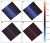 |
Fig. A.1. Background subtraction of the PSF matched F225W frame after the second iteration. (1): Raw data. (2): Computed background. (3): Background-subtracted data. (4): Uncertainties on the background. All panels share the same color cuts, selected to emphasize structure in the background. |
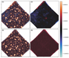 |
Fig. A.2. Example background subtraction of the PSF-matched F775W frame. Panel content is the same as in fig. A.1, except the upper and lower color cuts are half those of the fig. A.1. |
Fig. A.2 shows the same process, but for the F775W filter. Here, sources are more numerous and much brighter in comparison with the background. Additionally, giant elliptical galaxies with their old, red and UV-faint stellar populations are becoming visible in these bands. These galaxies have a substantially larger extent than the UV sources in F225W above, meaning that to avoid modeling and subtracting them, either a larger kernel or wider masks around detected sources are necessary. But these masks cannot be too wide, either, as the large number of small and faint sources in the field would leave very few pixels with which to model the background.
Panel (2) in fig. A.2 shows one such giant elliptical that has not been entirely masked out, such that the low surface brightness outer parts have been modeled and subtracted. This was the best compromise we could find between masking and leaving pixels to model without resorting to manual masking. We have checked if any of our sources are affected by this (weak) effect, which was not the case.
Appendix B: Source detection and deblending settings
B.1. Source detection settings
For each of the UV filters F225W, F275W and F336W, we ran the photutils source detection function detect_sources with a set of parameters selected to find all sources above a set of threshold values of signal-to-noise, Due to the comparatively low S/N in the UV filters, and the blotchy noise patterns described above, it can be difficult to distinguish spurious detections from real sources in each individual detection filter. At later steps, however, we have imaging data in up to ten additional filters available, meaning that we have opted for a set of very permissive source finding and detection settings, deliberately resulting in a large number of spurious detections that we then subsequently reject using the additional information provided by the additional data. In order to not miss any real but faint objects, we deliberately selected the detection parameters to allow for spurious detections. These could then be filtered out in subsequent steps based on optical and IR photometry in the segmentation maps. We found a set of suitable parameters for source detection and deblending by trial and error, eventually settling on the values tabulated in Table B.1.
Detection and deblending parameters used in the three detection filters.
B.2. Deblending
In deblending autodetected sources, one must strike a balance between on one hand separating truly distinct sources, while on the other hand correctly identifying substructure within a galaxy as such. The main purpose of deblending in the context of this work has been to correctly identify as many sources as possible at redshifts 2–4. We have therefore, as with source detection, pursued a quite aggressive deblending strategy, where correctly identifying unresolved or barely resolved but potentially overlapping sources took priority. This resulted in a number of clumps in large spirals identified as separate sources, but these were easily identified and rejected at later steps (see Sect. 3.5, especially 3.5.3).
A different challenge was posed by the blotchy pattern described in sect. 3.2. These patterns are sometimes difficult to tell apart from lower surface brightness extended features, and thus a balance needed to be found between on one side recovering all flux from true physical sources, while on the other hand avoiding including in the segmentation maps blotches that are too extended.
Parameters for source detection and deblending were set in a process of trial and error, and the final choices are presented in Table B.1.
In table B.1 we tabulate parameters passed to the photutils functions detect_sources and deblend_sources. Most are identical for the three filters but listed for completeness and ease of access. The process is described in sect. B.2. FWHM is the width in pixels of the Gaussian convolution kernel used for deblending; npixels is the minimum number of consecutive pixels required to be above the threshold S/N. Nlevels and contrast are explained in the photutils documentation.
B.3. Number of spurious detections
When detecting sources, we have deliberately set the detection criteria to be permissive, allowing for a relatively large number of spurious detection and relying on later filtering steps to discern these from real objects. This of course raises a concern regarding how effective these filtering steps are. With sufficiently many spurious detections present, the probability grows that some of these might slip through the filtering mechanisms set up to catch them.
We tested the magnitude of this problem by inverting the sign of the pixels in the background-subtracted F225W detection frame, and running the source detection routine with the exact same settings as before. By giving all true sources negative flux, we ensured that all detections were due to noise. We then proceeded as previously, by extracting flux from the neighboring filter on the red side, in this case F275W, in the segments created by the detection routine, and comparing colors and S/N as described for the science frames above, to test how large a fraction of the initial detections made it past these filtering criteria.
In the inverted F225W frame, we found 2317 “sources” living up to our detection criteria. After extracting the corresponding fluxes in F275W and comparing S/N and demanding that the AB magnitude be larger in the bluer band, we found that 18 of these sources still remained. We then tested these against the R15 and I17 catalogs with the same angular distance requirement of  as above; 5 of the 18 sources still remaining fell inside this radius of a catalog object, yielding a spurious detection rate of 5/2317, or 0.2%, before visual inspection.
Appendix C: UV filter error estimates
We ran the source detection routines in all the three UV filters. For each of these, we measured fluxes for every segment in the resulting segmentation filters in all 11 available filters. Visual inspection of a number of sources made us suspect that the errors in the UV filters were over estimated, which we confirmed by running Monte Carlo sampling, as described in the main text.
In fig. C.1, we show as an example the originally measured and the reestimated flux errors from the catalog detected using F275W. Objects with source sums ≲ 10-3, and typical S/N of ∼ 1, are spurious detections in F275W and are filtered out of our sample at the next step.
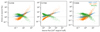 |
Fig. C.1. RMS map based (blue) and MC computed (orange) errors (×1020) plotted vs. aperture fluxes for the source catalog detected using F275W. The ratio between the two is shown in green for easier comparison. |
At the lowest fluxes, the errors are overestimated by a factor of ∼ 5–6. For brighter objects, this difference declines until the reestimated errors become higher than those based on the RMS map.
Appendix D: Rest-frame filter wavelength coverage
In Table D.1, we show the rest-frame wavelength coverage of each UV filter at the redshifts of each of the seven candidates. We are quoting the wavelengths from 1%–99% of the integrated dimensionless throughput of each filters as sampled in the software package PYSYNPHOT (STScI Development Team 2013).
Rest-frame UV filter wavelength coverage for each candidate.
Appendix E: Artifact in PSF matched F336W image
Our source detection picked up an apparent feature in F336W ∼1″ from F336W-1041. The feature is offset from the I17 and R15 catalog coordinates of the companion galaxy and, as is visible in fig. E.1, also from the flux centroid in the optical frames (here F775W). We inspected the non-PSF-matched archival frame as found in MAST and found that there was no source at that location in that filter. We thus suspect that the feature is an artifact of the PSF matching process.
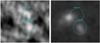 |
Fig. E.1. Cutouts of F336W-1041 (lower circle) and F336W-1043 (upper circle) in the filters F336W (left panel) and F775W (right panel). The circles are of arbitrary size. The upper feature in F336W is visibly offset from the upper feature in F775W, which is true for the rest of optical and IR data. In contrast, the spatial coincidence of the lower feature in the two filters is clear. |
To test whether the measured ionizing flux in 1041 could likewise be an artifact, we extracted the flux from a circular aperture matching the one used above and measured the flux and uncertainty. The values we recovered for both flux and uncertainty were consistent with the ones previously found, and its centroid in F336W coincident with that in the optical filters, so we conclude that this feature was real.
All Tables
Segment-measured AB magnitudes for the candidate objects in the five bluest filters in the UVUDF.
Parameters for background subtraction and source mask creation listed for each filter.
All Figures
|
Fig. 1. Approximate footprints of the combined MUSE-Deep cubes superimposed on the UVUDF FOV, represented by the PSF matched F275W frame. Colors to help distinguish individual MUSE pointings and mosaics. |
| In the text | |
|
Fig. 2. Filter throughput curves for the three detection filter plus F435W. For each detection filter, we also show the approximate lower redshift cut-off for galaxies to be reliably detected in LyC. Verification of detections in any filter is done in the filter immediately to the right. |
| In the text | |
|
Fig. 3. Spectral regions around rest-frame Lyα of the subset of candidate objects with Lyα in emission. At the bottom is shown the observed wavelength scale, above each panel is the corresponding rest-frame wavelength range. |
| In the text | |
|
Fig. 4. Postage stamp images in the filters F225W-F775W of the candidate objects, as well as a composite image of F435W, F606W and F775W for each candidate. The detection segment and the larger photometric aperture are shown in green in F606W as well as in the detection filter for each candidate. The reddest LyC-dominated filter is framed in thick black dashes for each candidate, and contours of the brightness in F775W are shown in F225W to provide a morphological comparison between the rest-frame far- and near-UV bands. The cut-outs are 2.7″ on a side. |
| In the text | |
|
Fig. 5. Spectral energy distributions of the leaker candidates, extracted in circular apertures of radius |
| In the text | |
|
Fig. 6. Segment fluxes (blue) and fixed-aperture fluxes (empty circles with the flux scale on the right) shown with BAGPIPES posterior photometry (orange dots) and model spectra (gray shading). |
| In the text | |
|
Fig. 7. Dust-, ISM-, and IGM-corrected model spectra of the candidates, as well as observed (filled circles) and model predicted (open circles). Orange spectra are the BAGPIPES best fit to the observed data points. Model spectra generated from the same best-fit parameters, but with ISM and dust removed, are shown in black. Gray spectra show the ISM- and dust-free model spectra corrected for the BAGPIPES assigned average redshift-dependent IGM absorption. |
| In the text | |
|
Fig. 8. Ionizing volume emissivity derived from the galaxies of this work compared to other measurements and predictions in the literature. Gray dashed and dotted lines show the theoretical models for bright AGN by Faucher-Giguère (2020) and Haardt & Madau (2012), and the fully drawn line shows the combined model of AGN and star formation from Faucher-Giguère (2020). Light green plus signs show the ionizing field in various redshift bins measured from the IGM properties by Becker & Bolton (2013). Dark green diamonds show the emissivity from star formation measured by Jones et al. (2021), and the single dark cross shows the estimate from Steidel et al. (2018). The filled orange marker shows the value derived from only the four tier one candidates in this work, while the open orange marker shows the value derived assuming that all the candidates are bona fide leakers. The open yellow marker shows the same as the open orange marker, but not corrected for IGM absorption. The orange and yellow markers are showed a bit offset on the redshift axis for visibility, but all are measured in one single redshift bin of 2 < z < 3.5 (illustrated with the horizontal yellow bar), with an average redshift of 2.81. |
| In the text | |
|
Fig. A.1. Background subtraction of the PSF matched F225W frame after the second iteration. (1): Raw data. (2): Computed background. (3): Background-subtracted data. (4): Uncertainties on the background. All panels share the same color cuts, selected to emphasize structure in the background. |
| In the text | |
|
Fig. A.2. Example background subtraction of the PSF-matched F775W frame. Panel content is the same as in fig. A.1, except the upper and lower color cuts are half those of the fig. A.1. |
| In the text | |
|
Fig. C.1. RMS map based (blue) and MC computed (orange) errors (×1020) plotted vs. aperture fluxes for the source catalog detected using F275W. The ratio between the two is shown in green for easier comparison. |
| In the text | |
|
Fig. E.1. Cutouts of F336W-1041 (lower circle) and F336W-1043 (upper circle) in the filters F336W (left panel) and F775W (right panel). The circles are of arbitrary size. The upper feature in F336W is visibly offset from the upper feature in F775W, which is true for the rest of optical and IR data. In contrast, the spatial coincidence of the lower feature in the two filters is clear. |
| In the text | |
Current usage metrics show cumulative count of Article Views (full-text article views including HTML views, PDF and ePub downloads, according to the available data) and Abstracts Views on Vision4Press platform.
Data correspond to usage on the plateform after 2015. The current usage metrics is available 48-96 hours after online publication and is updated daily on week days.
Initial download of the metrics may take a while.