© The Authors 2023

1. Introduction

The magnetic field of the solar corona must be studied because of its effects on and interactions with the plasma structures of the corona and because of the events resulting from temporal and spatial changes in this magnetic field. In the solar corona, structures are mainly formed and evolved in accordance with the magnetic field, and other forces such as pressure gradient and gravitational and dissipative forces can be ignored. The dynamics and topology of the solar corona are revealed by specifying the magnetic field configuration. However, the magnetic field in the solar corona can currently not be determined because the thermal broadening of the Zeeman lines swamps the magnetic broadening (Wiegelmann et al. 2006). The magnetic field in the solar corona is often reconstructed through extrapolation of magnetogram data (Schou et al. 2012a; Wiegelmann et al. 2012). Therefore, our physical knowledge of the coronal phenomena is mainly based on the reconstruction of the magnetic field that is directly measured in the solar photosphere. Several models have been developed for this purpose so far. They are based upon the simplified fact that the structures of the solar corona follow the rules of force-free magnetic fields. Therefore, it is assumed that the electric currents in the corona are aligned in the direction of the magnetic field, and measuring these currents is a good way of testing the success of the models of magnetic field reconstruction in the solar corona. This issue is discussed in Sect. 2. Thus, it is expected that the Lorentz force should vanish in the solar coronal medium, which is the domain of the magnetic field, B ≡ B(x, y, z),

$$\begin{array}{c}\hfill (\mathbf{\nabla }\times \mathit{B})\times \mathit{B}=0,\end{array}$$(1)

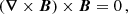
where x, y, z denotes the space coordinates. In the solar corona, the magnetic field must also be solenoidal as

$$\begin{array}{c}\hfill \mathbf{\nabla }·\mathit{B}=0.\end{array}$$(2)

A simple solution to the above equations is

$$\begin{array}{c}\hfill \mathbf{\nabla }\times \mathit{B}=\alpha (r)\mathit{B},\end{array}$$(3)

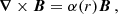
where α(r) is the force-freeness parameter and in general is a scalar function of the spatial coordinates, which is zero for potential fields, constant for linear force-free fields, and a scalar function of the spatial coordinates for nonlinear force-free magnetic fields. Since no general solution exists for Eqs. (1) and (2), Low & Lou (1990) applied a semi-analytical solution to these equations (hereafter L&L). In addition, several numerical models have been proposed to reconstruct the magnetic field (Grad & Rubin 1958; Inhester & Wiegelmann 2006; Amari et al. 1997, 1999; Wheatland et al. 2000; Wiegelmann 2004; Wiegelmann et al. 2005a,b; Yan & Sakurai 1997, 2000). A comprehensive review of the models for reconstructing force-free magnetic fields can be found in Wiegelmann & Sakurai (2021). A comparison of different models of magnetic field reconstruction was also offered by Schrijver et al. (2006). The optimization model developed by Wheatland et al. (2000) has received more attention (hereafter referred to as WSR). The WSR model has frequently been revised. For instance, Wiegelmann (2004) modified the optimization model by considering a weighting function (hereafter denoted OWF) and adding an additional layer to the top and lateral side boundaries. Wiegelmann et al. (2012) added an integral term to the Lagrangian containing the measurement errors of SDO/HMI¹ magnetogram and used a constant Lagrange multiplier to account for the injection speed of the boundary conditions and measurement errors in the reconstruction of the magnetic field. Wiegelmann & Neukirch (2006) applied the optimization principle to compute magnetohydrodynamic equilibria in the solar corona. Zhu & Wiegelmann (2018) examined the optimization model to study magnetohydrostatic equilibria. Inhester & Wiegelmann (2006) compared the WSR optimization and Grad-Rubin model by implementing the finite-element grid method and discussed the issue of gridding in optimization. The WSR optimization model is currently more popular because it facilitates computations, is easy to understand, and is cost-effective. As another approach to the optimization model, Nasiri & Wiegelmann (2019) employed the Lagrange multiplier technique to develop a constrained optimization model that is referred to as the constrained optimization by the scalar Lagrange multiplier function (COS). Several applications of constrained optimization techniques in different physical problems are briefly mentioned in Krishna Vadlamani et al. (2020). Furthermore, Bertsekas (1996) discussed different mathematical forms of the Lagrange multiplier models, the optimization principles, and the constrained optimization. The Lagrange multiplier technique is not merely confined to constant coefficients; rather, in general, it could be any scalar or vector function of space and time (Bertsekas 1996; Polyak 1969).

In Sect. 2, an appropriate Lagrangian is introduced, considering Eq. (1) as the constraint equation by a vector Lagrange multiplier. In Sect. 3, a brief review of the comparison models and the test case is provided. In Sect. 4, our algorithm is introduced. In Sect. 5, by optimizing the Lagrangian given in Sect. 2, a nonlinear force-free field is obtained. Furthermore, the results of the model are compared with those of the L&L semi-analytical solution and comparison models. Finally, the model is applied to a real vector magnetogram including active region (AR) 11 543. Section 6 is devoted to concluding remarks.

2. Theoretical approach

As mentioned in the introduction, the optimization models are easy to implement and have the advantage of computational efficiency. In the WSR model and in the relevant optimization methods, an appropriate Lagrangian is suggested to reconstruct a force-free field in the solar corona. In the COV model (Constrained Optimization with the Vector Lagrange multiplier), as an extension of the COS approach, we seek to use the optimization principle by employing a vector Lagrange multiplier to reconstruct the nonlinear force-free field. This is done by considering Eq. (2) as the governing equation of solenoidal nature and Eq. (1) as the constraint fixing the force-freeness nature of the magnetic field. By minimizing the term |∇ ⋅ B| subject to the constraint (∇ × B)×B = 0 using the Lagrange multiplier technique, the corresponding Lagrangian is then introduced as

$$\begin{array}{c}\hfill \begin{array}{c}{L}_{\mathrm{COV}}=L_{\mathrm{d}}+L_{\mathrm{f}}=\hfill \\ \hfill \\ {\int }_v{\omega }_{\mathrm{d}}{|\mathbf{\nabla }·\mathit{B}|}^2\mathrm{d}v+{\int }_v{\omega }_{\mathrm{f}}(\mathit{\lambda }·[(\mathbf{\nabla }\times \mathit{B})\times \mathit{B}])\mathrm{d}v,\hfill \end{array}\end{array}$$(4)

where ω_d and ω_f are weighting functions, and the indices d and f refer to divergence-free and force-free functions, respectively. In the same manner as in the COS model, B ≡ B(x, y, z, t) and λ ≡ λ(x, y, z, t) denote the magnetic field and the vector Lagrange multiplier, respectively. The Lagrange multiplier is used as a vector field because of the vector behavior of the constraint equation in Lagrangian of Eq. (4). The scaler nature of the Lagrange multiplier in the COS model was due to the scalar behavior of the corresponding constraint equation (∇ ⋅ B = 0). As a result, both terms in Eq. (4) become scalar quantities. The dimensional analysis in Eq. (4) shows that the dimension of the integrand in the first term is $\sim \frac{B^2}{l^2}$ and that of the second term is $\sim \frac{B^2}{l}$, meaning that |λ| has the dimension $\sim \frac{1}{l}$, where l has the dimension of length.

Taking the derivative of Eq. (4) and using appropriate vector algebra, we may obtain

$$\begin{array}{cc}\hfill \frac{\partial L_{\mathrm{COV}}}{\partial t}& ={\displaystyle {\int }_v[(\frac{\partial \mathit{B}}{\partial t}·{\mathit{F}}_{\mathrm{COV}}(\mathit{B},\mathit{\lambda }))+(\frac{\partial \mathit{\lambda }}{\partial t}·{\mathit{H}}_{\mathrm{COV}}(\mathit{B},\mathit{\lambda }))]\mathrm{d}v}\hfill \\ \hfill & +{\displaystyle {\int }_s(\frac{\partial \mathit{B}}{\partial t}·{\mathit{G}}_{\mathrm{COV}}(\mathit{B},\mathit{\lambda }))\mathrm{d}s,}\hfill \end{array}$$(5)

where

$$\begin{array}{cc}\hfill {\mathit{F}}_{\mathrm{COV}}(\mathit{B},\mathit{\lambda })& ={\omega }_{\mathrm{f}}(\mathit{\lambda }\times (\mathbf{\nabla }\times \mathit{B}))+{\omega }_{\mathrm{f}}(\mathbf{\nabla }\times (\mathit{B}\times \mathit{\lambda }))\hfill \\ \hfill & +\mathbf{\nabla }{\omega }_{\mathrm{f}}\times (\mathit{B}\times \mathit{\lambda })-2[(\mathbf{\nabla }·\mathit{B})\mathbf{\nabla }{\omega }_{\mathrm{d}}+{\omega }_{\mathrm{d}}\mathbf{\nabla }(\mathbf{\nabla }·\mathit{B})],\hfill \end{array}$$(6)

$$\begin{array}{c}\hfill {\mathit{G}}_{\mathrm{COV}}(\mathit{B},\mathit{\lambda })=2{\omega }_{\mathrm{d}}(\mathbf{\nabla }·\mathit{B})\mathit{n}+(\mathit{B}\times \mathit{\lambda })\times {\omega }_{\mathrm{f}}\mathit{n},\end{array}$$(7)

and

$$\begin{array}{c}\hfill {\mathit{H}}_{\mathrm{COV}}(\mathit{B},\mathit{\lambda })={\omega }_{\mathrm{f}}[(\mathbf{\nabla }\times \mathit{B})\times \mathit{B}].\end{array}$$(8)

The details of the above calculations are shown in Appendix A. To reconstruct the field over an active region, we assumed a box whose bottom side coincides with the given magnetogram, while the lateral and top sides are in the solar corona. We reconstructed the magnetic field inside the box by extrapolating the photospheric field. Assuming that no active region is located near the edges of the magnetogram, we expect that the magnetic field of the lateral boundaries of the box remain constant throughout the optimization procedure; that is,

$$\begin{array}{c}\hfill {\left(\frac{\partial \mathit{B}}{\partial t}\right)}_s=0.\end{array}$$(9)

Therefore, the surface integral in Eq. (5) vanishes. The volume integrals in Eq. (5) will always be negative assuming

$$\begin{array}{c}\hfill \frac{\partial \mathit{\lambda }}{\partial t}=-{\mu }_1{\mathit{H}}_{\mathrm{COV}}(\mathit{B},\mathit{\lambda }),\end{array}$$(10)

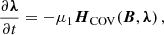
and

$$\begin{array}{c}\hfill \frac{\partial \mathit{B}}{\partial t}=-{\mu }_2{\mathit{F}}_{\mathrm{COV}}(\mathit{B},\mathit{\lambda }),\end{array}$$(11)

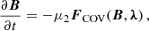
where μ₁ and μ₂ are positive parameters to be specified during the numeric calculations. It should be noted that in the above equations, μ₁ and μ₂ have the dimensions of $\frac{1}{B^2}$ and l², respectively. Using Eqs. (10) and (11) in Eq. (5), we may obtain the following explicit form:

$$\begin{array}{c}\hfill \frac{1}{2}\frac{\partial L_{\mathrm{COV}}}{\partial t}=-{\displaystyle {\int }_v({\mu }_1|{\mathit{H}}_{\mathrm{COV}}{(\mathit{B},\mathit{\lambda })|}^2+{\mu }_2|{\mathit{F}}_{\mathrm{COV}}(\mathit{B},\mathit{\lambda }){|}^2)\mathrm{d}v.}\end{array}$$(12)

The minimization mechanism inherent in Eq. (12) means that an arbitrary λ can be chosen, as well as B as an initial input, and their evolution can be followed through the coupled Eqs. (10) and (11). The final task is to find the magnetic field satisfying the appropriate boundary conditions, therefore we used a potential magnetic field(B₀) as the input field and a suitable ansatz for the initial value of the λ in terms of B₀ as follows:

$$\begin{array}{c}\hfill \mathit{\lambda }\equiv {\mathit{\lambda }}_{\mathbf{0}}={|{\mathit{B}}_{\mathbf{0}}|}^{-2}[(\mathbf{\nabla }\times {\mathit{B}}_{\mathbf{0}})\times {\mathit{B}}_{\mathbf{0}}].\end{array}$$(13)

Therefore, starting with a positive L_COV, it will eventually approach zero at the end of the iteration. The Lagrange multiplier, λ, and the magnetic field, B, were updated simultaneously at each iteration step according to Eqs. (10) and (11), respectively. Thus, following the optimization procedure, we may reconstruct the expected divergence-free and force-free output magnetic field by the COV model to the extent that the boundary conditions are consistent.

3. Comparison models and test case

To verify the performance of our model, we compared the corresponding results with those obtained by other models, preferably with the results of any possible exact solution. By assuming a point source at the origin, Low & Lou solved Eqs. (1) and (2) and provided a set of axisymmetric nonlinear force-free fields. This set of semi-analytical solutions has a multipolar character based on the depth of burying the origin below the photosphere (l) and the inclination of the axis of symmetry of the fields to the normal (ϕ). The semi-analytical solutions that are labeled in the L&L notation P_1, 1 with l = 0.3, and ϕ = π/4, were selected as a test case, and the corresponding vector magnetic field was generated for all cells in the box in which the magnetic field was reconstructed. Then, the results of the COV model were compared with the result of the test case (L&L), as well as those of the WSR, OWF, and COS models.

In the WSR model, the required equations are obtained by minimizing the following Lagrangian:

$$\begin{array}{c}\hfill L_{\mathrm{WSR}}={\displaystyle {\int }_v}{(|\mathbf{\nabla }·\mathit{B}|}^2+{|\mathit{B}|}^{-2}{[(\mathbf{\nabla }\times \mathit{B})\times \mathit{B}]}^2)\mathrm{d}v.\end{array}$$(14)

As noted by Wheatland et al. (2000), one of the main conditions of optimizing Eq. (14) is to use the boundary condition (∂B/∂t)_s = 0, which assumes that the magnetic field on all sides of the computational box remains unchanged during the iteration. Nevertheless, it is not appropriate to use this condition abruptly on the boundaries of the box, and therefore Wiegelmann (2004) optimized the Lagrangian L_OWF by multiplying the weighting functions by the integrand as

$$\begin{array}{c}\hfill L_{\mathrm{OWF}}={\displaystyle {\int }_v({\omega }_{\mathrm{d}}{|\mathbf{\nabla }·\mathit{B}|}^2+{\omega }_{\mathrm{f}}{|\mathit{B}|}^{-2}{[(\mathbf{\nabla }\times \mathit{B})\times \mathit{B}]}^2)\mathrm{d}v,}\end{array}$$(15)

where ω_d and ω_f are the weighting functions for the divergence-free and force-free terms, respectively. Another comparison model is the constrained optimization model (COS) developed by Nasiri & Wiegelmann (2019), which uses a scalar function as a Lagrange multiplier. The corresponding Lagrangian is

$$\begin{array}{c}\hfill L_{\mathrm{COS}}={\displaystyle {\int }_v({\omega }_{\mathrm{d}}\lambda (\mathbf{\nabla }·\mathit{B})+{\omega }_{\mathrm{f}}{|\mathit{B}|}^{-2}{[(\mathbf{\nabla }\times \mathit{B})\times \mathit{B}]}^2)\mathrm{d}v.}\end{array}$$(16)

The divergence-free condition of Eq. (2) is considered as a constrained equation, and λ is the scalar function serving as a Lagrange multiplier due to the scaler nature of the constrained equation. In other words, if the constrained equation is scalar, the corresponding Lagrange multiplier becomes a scalar function. Otherwise, if the constrained equation is a vector, the corresponding Lagrange multiplier becomes a vector field.

4. Algorithm

As mentioned in the previous sections, to reconstruct the magnetic field in the solar corona, the model was run on th5e computational box, whose bottom side is located in the photosphere. We describe the steps below.

1. The magnetogram (artificial or real) was selected in such a way that its edges were sufficiently far from the active regions and was used as the boundary condition at the lower side of the box. Therefore, to test the model, the magnetic field generated by the L&L semi-analytical solution was used as an artificial magnetogram. Since the L&L solution was calculated from force-free magnetic field equations, the boundary conditions would be in accordance with the force-free conditions. In real cases, preprocessed boundary data must be used by controlling the smoothing and removing high noise levels, ambiguities, and the effect of the non-force-free magnetic field at the coronal base for consistency between the model and the boundary data (Wiegelmann et al. 2006, 2015; Schrijver et al. 2006; Fuhrmann et al. 2011; Tadesse et al. 2009). The procedure of the optimization code is similar for artificial or real magnetograms.

2. The potential magnetic field configuration was used as an input field, and its values on the lateral and top sides were used as a boundary condition in an iterative technique. By solving Eq. (3) through Green’s function method, the potential field was calculated for the entire box (Seehafer 1978). For this purpose, the potential field can be obtained by using the vertical components of the magnetic field at the bottom side of the box, assuming α = 0 and B_z to vanish at the side boundaries and fixing the expansion coefficients by the (real or artificial) magnetogram. The assumption about B_z arises because the potential field is obtained by the normal component of the magnetic field, which is smaller at the boundary than the values in the inner parts of the box.

3. λ may assume a finite value that can minimize L. Thus, we only need λ to converge to a finite value. Therefore, we defined the Lagrange multiplier in terms of the potential magnetic field as Eq. (13) at the first iteration step and used it as the input of the evolution Eq. (10). For the next step, λ was updated according to Eq. (10). According to Eq. (9) the boundary value for the magnetic field was fixed during the iteration procedure, while the boundary condition for λ was updated according to Eqs. (10) and (9), and at any step of the iteration, λ|_s served as the boundary condition for the next iteration step.

4. Finally, using Eqs. (10) and (11), we iterated and updated both the Lagrange multiplier and the magnetic field inside the computational box. This was done by starting with a positive L_COV, and according to Eq. (12), the Lagrangian eventually tends toward zero and the expected force-free and divergence-free magnetic fields were obtained as far as the boundary conditions permit.

The algorithm was implemented using the code provided in Wiegelmann (2017) and by developing according to the respective terms of the COV model. Some notes on the boundary values of λ are given in the next section.

We assumed that μ₁ and μ₂ were equal to one at the beginning of the optimization. Following the same procedure as Wiegelmann (2004), μ₁ and μ₂ change during the optimization according to the behavior of the converging quantities and the error caused by the numerical calculations. Here, if the criterion L_t + 1 < L_t was not satisfied during the numerical calculations, μ₁ and μ₂ were reduced by a factor of 0.5. Then, to guarantee convergence, both of these parameters were slowly increased by a factor of 1.01 in each step.

Furthermore, the boundary values on all six sides of the box are expected to be matched smoothly with the interior force-free magnetic field. Thus, additional boundary layers were considered for the lateral and top sides of the box. We assumed two different values n_d = 0 and 8 for the thickness of the layer. The inner box is called the physical box, and the outer one is called the computational box (Wiegelmann 2004). For n_d = 8, the weighting function is equal to one inside the box and decreases monotonically to zero across the boundary layer by assuming a cosine profile, while for n_d = 0, the weighting function is equal to one throughout the box. We compared our results with those of WSR, OWF, and COS models for both n_d = 0 and 8.

5. Numerical analysis

It is well known that nonlinear force-free reconstruction models do not relax to a force-free state, even using the weighting function approach of Wiegelmann (2004) to reduce the boundary mismatches (De Rosa et al. 2009). This is due to different factors such as the lack of top and sides boundary data, the inconsistency of the boundary condition of B_z (or α) with a nonlinear force-free magnetic field over the two polarities of B_z, the errors in the magnetogram measurements, and deviations in the photospheric magnetic field from the nonlinear force-free magnetic field (De Rosa et al. 2015, 2009). The convergency considered here is reliable insofar as the above problems are fulfilled. Nevertheless, the highest possible consistency of the force-free magnetic field with the given boundary data should be aimed for. Preprocessing the measured vector magnetograms serves this aim, and is applied to real magnetogram data in Sect. 5.4. However, we first apply the COV model to the L&L semi-analytical solutions as an artificial magnetogram.

5.1. Applying the model to an artificial magnetogram

We selected a set of L&L semi-analytical solutions, as mentioned in Sect. 3 and generated the vector magnetic field by the L&L solutions for all grid cells. The corresponding values for the bottom side of the box were used as an artificial vector magnetogram and as the boundary condition in reconstructing the magnetic field in the solar corona. Next, the potential field was calculated using the boundary conditions mentioned above and was employed as input for the optimization procedure. The box assumed over the active region was divided into 80 segments along the x- and y-axes and into 72 segments along the z-axis. The lateral boundaries of the box were selected in such a way that no active region would lie close to the boundaries, so that Eq. (9) is satisfied.

Equations (10) and (11) were solved by iteration procedure, and the nonlinear force-free field was obtained after 4000 iteration steps. The results of L/L₀ for the COV, COS, OWF, and WSR models are shown in Fig. 1 in an iteration step t = 4000 for n_d = 0 and n_d = 8, respectively. After 4000 iteration steps, the value of L_COV(B, λ) approaches ∼0.003 and ∼0.0003 of its initial value (L₀(B, λ)) for n_d = 0 and n_d = 8, respectively. As shown in Fig. 1, a relatively better convergence of COV in the initial steps may be an advantage of our model. This feature is particularly useful in problems that require the reconstruction of fields for a considerable number of time series of magnetograms, which may be done with a few hundred iteration steps because the computational time is limited. The reason for this convergence may be that the vector Lagrange multiplier is coupled with the Lorentz force term, which contributes more than the solenoidal term in Eq. (4). The normalized value of the force-free term in a computational analysis starts from ≃64.25, while the divergence-free term starts from ≃4.47 for n_d = 8.

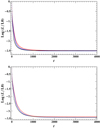Fig. 1. Iterative behavior of the normalized value of the Lagrangian, $\frac{L(\mathit{B},\mathit{\lambda })}{L_0(\mathit{B},\mathit{\lambda })}$, in logarithmic scale. Top: Results for nd = 0 are shown as a black line for LCOV, a red line for LCOS, and a blue line for LWSR. Bottom: Results for nd = 8 shown as a black line for LCOV, a red line for LCOS, and a blue line for LOWF.

As mentioned before, in a medium embedded in a force-free magnetic field, the electric current density vector would align itself with the magnetic field (Wiegelmann & Sakurai 2021). We therefore defined

$$\begin{array}{c}\hfill {\sigma }_i\equiv sin{\theta }_i=\frac{{|\mathit{J}\times \mathit{B}|}_i}{J_i{B}_i},\end{array}$$(17)

where the index i denotes the grid number within the computational box, which assumes the values 1 up to 80 * 80 * 72 = 460 800, and θ_i is the angle between the corresponding J and B. Then, we defined the current-weighted value of the angle between the current density vector and the magnetic field, θ_J, as follows (Wheatland et al. 2000):

$$\begin{array}{c}\hfill {\sigma }_J=\frac{{\sum }_i{J}_i{\sigma }_i}{{\sum }_i{J}_i}=sin{\theta }_J.\end{array}$$(18)

θ_J is plotted versus the iteration parameter t in Fig. 2 for the COV, COS, OWF, and WSR models. The force-free magnetic field is reconstructed by a relatively rapid convergence in the COV model, which is inherent in the behavior of the corresponding L/L₀ in Fig. 1.

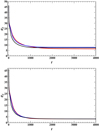Fig. 2. Iterative behavior of θJ during the optimization. Top: Results for nd = 0 shown as a black line for LCOV, a red line for LCOS, and a blue line for LWSR. Bottom: Results for nd = 8 shown as a black line for LCOV, a red line for LCOS, and a blue line for LOWF.

To show the convergence of the solenoidal term, we checked the histogram of the fractional, flux errors defined as

$$\begin{array}{c}\hfill f_i=\frac{{\int }_{△s_i}\mathit{B}·\mathit{ds}}{{\int }_{△s_i}|\mathit{B}|\mathrm{d}s}\approx \frac{{(\mathbf{\nabla }·\mathit{B})}_i(△V_i)}{B_i{A}_i},\end{array}$$(19)

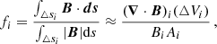
where the index i refers to the number of each cell in the computational box (Wheatland et al. 2000). In Fig. 3, the dispersion of the ⟨|f_i|⟩ is shown for the last iteration step t = 4000. For the COV model, ⟨|f_i|⟩ reaches ∼3.3 × 10⁻⁴, which is in agreement with and has the same order of magnitude as those of the OWF model, that is, ∼2.8 × 10⁻⁴, achieving a state close to the divergence-free magnetic field. In addition, after 4000 iteration steps, L_d reaches 0.059 and 0.008 for n_d = 0 and n_d = 8, respectively, which are less than 0.015 and 0.002 of their initial values.

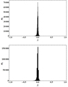Fig. 3. Histogram of the dispersion of the fractional flux error, ⟨|fi|⟩, around zero over all grid points for the last iteration step t = 4000. ni indicates the number of grid cells. Top: Results for nd = 0. Bottom: Results for nd = 8.

Examining the behavior of magnetic energy during optimization may be useful. It is known that the magnetic energy of a nonlinear force-free field in an active region is higher than that of a corresponding linear force-free and potential field (Jing et al. 2009; De Rosa et al. 2015; Wiegelmann et al. 2012). Since the optimization procedure starts with a potential field and ends with a nonlinear force-free field, we expect that the magnetic energy content of the plasma increases during the optimization. The ratio of the magnetic energy to its initial value $\frac{E}{E_0}$ is plotted in Fig. 4, which shows the upper limit given in Table 1. This agrees with the results obtained by Wiegelmann et al. (2012), demonstrating the flaring process (Jing et al. 2008; Wiegelmann et al. 2012).

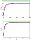Fig. 4. Behaviour of the ratio of the magnetic energy to its initial value during the iteration. The top plot shows LCOV (black), LCOS (red), and LWSR (blue) for nd = 0, and the bottom plot shows LCOV (black), LCOS (red), and LOWF (blue) for nd = 8. For nd = 8, we obtain a closer value to EL & L/Epotential (green dotted line) than for nd = 0.

Furthermore, to enhance our understanding of the models, a few magnetic field lines in the computational box are plotted in Figs. 5a–i for the potential, L&L, WSR, COS, OWF, and COV models.

Fig. 5. Reconstructed magnetic field lines for different models. (a) Artificial magnetogram in line-of-sight view. The color bar shows the strength (in Gauss) and polarity of the magnetic field. The reconstructed magnetic field lines are plotted for (b) the L&L semi-analytical solution, (c) the potential field, (d) theWSR optimization models, (e) the COS and (f) COV models without the weighting function, (g) the OWF optimization model, and (h) the COS and (i) COV models with a weighting function.

5.2. Indicator examination for the artificial magnetogram

For a quantitative comparison, the examination of indicators defined by Schrijver et al. (2006) may be useful for each model. These indicators are

(A) the relative magnetic energy, ϵ, defined as

$$\begin{array}{c}\hfill ϵ\equiv \frac{{\sum }_i|{\mathit{b}}_i^2|}{{\sum }_i|{\mathit{B}}_i^2|},\end{array}$$(20)

where b_i is the final nonlinear force-free field and B_i is the corresponding field for the L&L semi-analytical solution, and the summation goes over the grid numbers. This quantity shows the ability of the model to estimate the energy content of the reconstructed magnetic field. As listed in Table 1, the relative magnetic energy obtained in COV was 0.99 and 0.96 for n_d = 8 and n_d = 0, respectively, which is close to 1 and is compatible with the results of the WSR, OWF, and COS models.

(B) The normalized vector error, NVE, is defined as

$$\begin{array}{c}\hfill \mathrm{NVE}\equiv \sum _i\frac{|{\mathit{b}}_i-{\mathit{B}}_i|}{|{\mathit{B}}_i|}.\end{array}$$(21)

NVE shows the vector error normalized to the average vector norm and approaches zero when b_i and B_i are almost identical. As shown in Table 1, NVE for the COV model is more or less close to zero, as for other comparison models for a given n_d.

(C) The vector correlation, VC, is defined as

$$\begin{array}{c}\hfill \mathrm{VC}\equiv {\displaystyle \sum _i\frac{{\mathit{B}}_i{\mathit{b}}_i}{\sqrt{\sum _i|{\mathit{B}}_i^2|\sum _i|{\mathit{b}}_i^2|}}.}\end{array}$$(22)

It represents the correlation between B_i and b_i at each grid point i. In contrast to NVE, VC approaches unity when b_i and B_i are almost identical. As shown in Table 1, the VC obtained for COV is almost the same as in the other comparison models as well as in the L&L semi-analytical solution.

(D) Cauchy-Schwarz, CS, is defined based on Cauchy-Schwarz inequality as

$$\begin{array}{c}\hfill \mathrm{CS}\equiv \frac{1}{N}{\displaystyle \sum _i\frac{{\mathit{B}}_i·{\mathit{b}}_i}{|{\mathit{B}}_i||{\mathit{b}}_i|},}\end{array}$$(23)

where N denotes the total number of grid points in the computational box. This metric measures the angle between B_i and b_i. As shown in Table 1, the results of this quantity for n_d = 8 are better than those for n_d = 0 for all models, having the same order of magnitude. Therefore, the above indicators show that the results obtained are more or less the same for different models.

5.3. Notes about λ

According to the theory of the Lagrange multiplier technique, λ may serve as an appliance to minimize the constrained Lagrangian L. Thus, we expect that |λ| has a finite value, as shown in Fig. 6, otherwise, the Lagrangian L is undefined. The average value of λ starts with a finite value according to Eq. (13) and evolves according to Eq. (10). Since ⟨|δλ|⟩ approaches zero at the end of the iteration, λ will assume a finite value, as shown in Fig. 6.

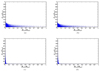Fig. 6. Iterative behavior of the average values of λ top) and ⟨|δλ|⟩ (bottom) for each iteration vs. t for an artificial magnetogram.

Another appealing point is the behavior of the average value of λ for each iteration. As shown in Fig. 6, the expression for the relative average value, |λ|/|λ_max|, by an artificial magnetogram first decreases for a few iteration steps and then increases with t, where |λ_max| is the maximum value of |λ| in the last iteration (t = 4000). To illustrate the iterative behavior of the Lagrange multiplier, we plot |λ| versus the magnetic field |B| during the optimization in Fig. 7, where the scattering of |λ_i|/|λ_max| versus |B_i|/|B_max| is plotted within all grid points of the computational box for four different snapshots (t = 1, 100, 1000, 4000), and B_max is the maximum value of B in the last iteration (t = 4000). It seems that as the iteration procedure continues, the vector Lagrange multiplier is stronger in regions with a weaker magnetic field. The grid cells with a large |λ| have a weaker magnetic field, while the grid cells with a stronger magnetic field have a small |λ|. Thus, the mean value of the |λ| is finally mainly formed by weaker regions. As the optimization proceeds, the magnetic field becomes localized and rearranged, and the number of grid points with a higher magnetic field intensity decreases, which leads to a rearrangement of |λ_i| in different grid points, as seen in Figs. 7a–d. This is due to the fact that the structure of the initial potential magnetic field is different from the final magnetic field of the box. As the iteration proceeds, the magnetic field rearranges itself to become compatible with the localized magnetic field of the active regions in the magnetogram and the corresponding magnetic field lines above, which occupies a small fraction of the grid cells of the box. Therefore, at the end of the iteration, a limited number of the grid points corresponding to the active regions will remain with strong magnetic fields. Except for a few initial iteration steps, λ therefore increases because according to Fig. 7, the number of grid points with the weaker magnetic field (larger lambda) increases while the number of those with the stronger magnetic field (smaller lambda) decreases during the iteration. However, because ⟨|δλ|⟩ approaches zero for large iteration numbers, lambda increases and approaches a finite value. This leads to the observed iterative behavior of |λ_i|/|λ_max| shown in Fig. 6.

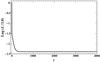Fig. 7. Scattering of |λ|/|λmax| vs. |B|/|Bmax| for (a) t = 1, (b) t = 100, (c) t = 1000, and (d) t = 4000 for all cells of the computational box.

5.4. Applying the model to a real vector magnetogram

To investigate the real condition, the model was applied to a vector magnetogram image of SDO/HMI, which provides a vector magnetic field with high spatial and temporal resolution in the solar photosphere (Schou et al. 2012b). To check the agreement with the assumptions of a force-free magnetic field, we performed preprocessing operations. These assumptions are known as the Aly criteria and must be fulfilled if a vector magnetogram is used as the photospheric boundary condition for nonlinear force-free modeling (Aly 1989). When these criteria are not met, the data must be preprocessed to become compatible with the model (Wiegelmann et al. 2006; Fuhrmann et al. 2011).

The magnetogram we used included the active region AR 11543 and was observed at 00 : 12 UT on 13 August 2012. It has 640 × 640 pixels with a spatial resolution of ≃370 km per pixel. The target area was selected in such a way that the edges of the image do not cross the active region and are located far enough from it. In addition, the active region is close to the center of the Sun in N20W07 so that the effects of the edge of the Sun are removed. To increase the speed of computation, we binned the data to 80 × 80 pixels. A reduced resolution will affect the calculated magnetic energy and decreases the metrics of the nonlinear force-free field, the current, and flux imbalance (De Rosa et al. 2015). The computational box was considered to have 80 pixel along the z-axis, and the thickness of the boundary layer was assumed as n_d = 4. To obtain an appropriate boundary condition on the magnetic field at the lower side of the box, the optimal preprocessing parameter set was calculated based on the minimizing technique of Eq. (6) in Wiegelmann et al. (2006). Several data sets have been presented in the literature to preprocess SDO/HMI data (Tadesse et al. 2013, 2011; Wiegelmann et al. 2012). However, we used the standard data set for the preprocessing parameters, μ1 = 1, μ2 = 1, μ3 = 0.001, μ4 = 0.01, as described by Wiegelmann et al. (2006) to correct the force freeness, the torque freeness, the optimized boundary matches with the photospheric data, and the smoothing, respectively. When the real magnetogram is optimized, the Lagrangian reaches 0.004 of its initial value after 4000 iteration steps. The iterative behavior of the Lagrangian L is shown in Fig. 8. In addition, the average value of the magnitude of the fractional flux errors, ⟨|f_i|⟩ was reached at 1.33 × 10⁻³ for the physical box, as shown in Fig. 9, indicating that the final state of the model for the real magnetogram is almost close to the divergence-free solution throughout the grid points. Furthermore, the current-weighted value of the angle between the current density and the magnetic field, θ_J, reduces from 59.06° and 56.69° at the beginning to 13.11° and 10.61° at the end of iteration for the computational and physical box, respectively. It may be useful to investigate the behavior of the magnetic energy for an observational magnetogram during the optimization. The relative total magnetic energy content to the potential one is calculated to be 1.185 in the box, as shown in Fig. 10. Thus, the free magnetic energy, E_free = E_F − E_P, inside the box is estimated to be 2.20 × 10²⁹ erg². Some of the closed reconstructed nonlinear force-free magnetic field lines are plotted over the given magnetogram in Fig. 11.

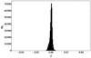Fig. 8. Iterative behavior of the normalized value of the Lagrangian, $\frac{L(\mathit{B},\mathit{\lambda })}{L_0(\mathit{B},\mathit{\lambda })}$, in logarithmic scale so that the COV model can be applied to the real magnetogram.

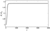Fig. 9. Distribution of fractional flux errors, ⟨|fi|⟩ around zero for the last iteration step over all grid points for the COV model using the real magnetogram.

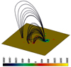Fig. 10. Behavior of the ratio of the total reconstructed and potential magnetic energy during the iteration for the real magnetogram.

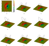Fig. 11. Nonlinear force-free field lines above the magnetogram obtained from the region containing AR 11543. The color bar shows the strength (in Gauss) and the polarity of the magnetic field of the magnetogram.

6. Conclusions

Force-free stable equilibria in the solar corona are a most interesting problem because most parts of the corona are magnetically confined, that is, the plasma-β parameters P_th/P_mag ≪ 1 (Gary 2001). The effect of nonmagnetic forces on the dynamical behavior of the corona, such as the pressure gradient and gravity forces, can therefore be ignored. Although this approximation is violated in lower atmospheric levels, the evolution of structures and the description of the events in the solar corona can be explained by the physics of force-free magnetic fields. Therefore, it is necessary to realize the configuration and aspects of the magnetic field in the solar corona. Because of the conditions in the corona as well as because of technical problems, direct measurements of the magnetic field in the solar corona are still impossible. Therefore, the magnetic field must be reconstructed using photospheric data obtained thorugh magnetograms. For this purpose, the Lagrange multiplier technique was applied to reconstruct a force-free magnetic field in solar corona conditions. The magnetic field was reconstructed inside a computational box over a given artificial and observational magnetogram. The initial potential magnetic field was obtained as a solution of the Laplace equation using Green’s function method and was fixed by the appropriate boundary conditions assumed for the normal component of the magnetic field by the same procedure as Seehafer (1978). In this model, the reconstruction was implemented by optimizing a Lagrangian constructed by a solenoidal field subject to the constrained equation governing a force-free magnetic field. Furthermore, by assuming the potential magnetic field for the lateral and top sides as well as magnetogram data (artificial or observational) as the boundary conditions for B, and using Eq. (13) to specify the initial value for λ, the iteration procedure was followed for the computational box to reconstruct the magnetic field. Like the other optimization models, the COV model also overprescribes. In this limitation, the boundary conditions prevent the convergence of the relevant quantities in the iteration process. The results are compared with those of the corresponding optimization models such as the WSR, OWF, and COS, and with the L&L semi-analytical solutions as a test case. The Lagrangian, and consequently, the angle between the electric current density and the magnetic field, approaches zero faster than that of comparison models at least for the initial iteration steps. This is an advantage of the model, which may be helpful for time-series events, while several magnetograms must be considered and limited iteration steps are needed. The results obtained by using the weighting function agree better than the result without the weighting function. The iterative evolution of the magnetic energy during optimization yields an upper limit for the magnetic energy, as expected when the nonlinear force-free field is reconstructed using a potential magnetic field as the input for the iteration procedure.

The Lagrangian in our method was constructed in a regulated procedure based on the Lagrange multiplier technique, which is facilitated first by fixing a physical divergence-free condition (L_d term), and subsequently, by adding the constrained equation (L_f term) by an appropriate vector Lagrange multiplier. Furthermore, the Lagrange multiplier technique is capable of including more general cases, where the force-free magnetic field may be a special case, and other constraints could be manipulated using the similar technique.

Because of the condition of mixed β in the photosphere and in the lower layers of the chromosphere, the effects of nonmagnetic forces in the lower parts of the computational box may cause the results to be inconsistent with real solar coronal data. The model is developed to include this condition, and the problem is currently under investigation.

Acknowledgments

The authors gratefully acknowledge the referee for carefully reading the manuscript and giving constructive comments and informative recommendations that substantially helped us to improve the quality and readability of the paper. One of the authors (S. Nasiri) would like to thank Thomas Wiegelmann for kindly providing us the optimization code when I was on sabbatical leave at the Max Plank Institute for Solar System Research (MPS).

References

Appendix A: Derivation of equation 5

Differentiating Eq. (4) with respect to the iteration parameter, we obtain

$$\begin{array}{c}\hfill \frac{\partial L_{\mathit{COV}}}{\partial t}={\displaystyle {\int }_v[2{\omega }_d[(\mathbf{\nabla }·\mathit{B})(\mathbf{\nabla }·\frac{\partial \mathit{B}}{\partial t})]+{\omega }_f[\mathit{\lambda }·((\mathbf{\nabla }\times \frac{\partial \mathit{B}}{\partial t})\times \mathit{B})]+{\omega }_f[\mathit{\lambda }·((\mathbf{\nabla }\times \mathit{B})\times \frac{\partial \mathit{B}}{\partial t})]+{\omega }_f[\frac{\partial \mathit{\lambda }}{\partial t}·((\mathbf{\nabla }\times \mathit{B})\times \mathit{B})]]dv.}\end{array}$$(A.1)

This integral includes four separate terms. We wish to perform each of these terms as a dot product with $\frac{\partial \mathit{B}}{\partial t}$ or with $\frac{\partial \lambda }{\partial t}$. The fourth term in Eq. (A.1) is already in the required form, but the other terms need some algebraic calculations to reach the desired form.

Considering the first term and using the vector identity ∇ ⋅ (ψA) = ψ(∇ ⋅ A)+A ⋅ ∇ψ, we obtain

$$\begin{array}{c}\hfill I_1\equiv 2{\displaystyle {\int }_v{\omega }_d(\mathbf{\nabla }·\mathit{B})(\mathbf{\nabla }·\frac{\partial \mathit{B}}{\partial t})dv=2{\int }_v\mathbf{\nabla }·[{\omega }_d(\mathbf{\nabla }·\mathit{B})\frac{\partial \mathit{B}}{\partial t}]dv-2{\int }_v\frac{\partial \mathit{B}}{\partial t}·\mathbf{\nabla }[{\omega }_d(\mathbf{\nabla }·\mathit{B})]dv.}\end{array}$$(A.2)

Applying the Gauss law to the second term on the right-hand side of Eq. (A.2), we obtain

$$\begin{array}{c}\hfill I_1=-2{\displaystyle {\int }_v\frac{\partial \mathit{B}}{\partial t}·({\omega }_d\mathbf{\nabla }(\mathbf{\nabla }·\mathit{B})+(\mathbf{\nabla }·\mathit{B})\mathbf{\nabla }{\omega }_d)dv+2{\int }_s\mathit{n}·\left({\omega }_d(\mathbf{\nabla }·\mathit{B})\frac{\partial \mathit{B}}{\partial t}\right)ds.}\end{array}$$(A.3)

Rearranging the second term, we obtain the desired form for the I₁ integral as

$$\begin{array}{c}\hfill I_1=-2{\displaystyle {\int }_v\frac{\partial \mathit{B}}{\partial t}·({\omega }_d\mathbf{\nabla }(\mathbf{\nabla }·\mathit{B})+(\mathbf{\nabla }·\mathit{B})\mathbf{\nabla }{\omega }_d)dv+2{\int }_s\frac{\partial \mathit{B}}{\partial t}·\left({\omega }_d(\mathbf{\nabla }·\mathit{B})\mathit{n}\right)ds.}\end{array}$$(A.4)

Furthermore, with the vector identities ∇ ⋅ (A × B) = B ⋅ (∇ × A)−A ⋅ (∇ × B) and A ⋅ (B × C) = B ⋅ (C × A), the second term in Eq. (A.1) becomes

$$\begin{array}{c}\hfill I_2\equiv {\displaystyle {\int }_v{\omega }_f(\mathit{\lambda }·(\mathbf{\nabla }\times \frac{\partial \mathit{B}}{\partial t})\times \mathit{B})dv={\int }_v{\omega }_f(\frac{\partial \mathit{B}}{\partial t}·(\mathbf{\nabla }\times (\mathit{B}\times \mathit{\lambda })))dv+{\int }_v{\omega }_f\mathbf{\nabla }·((\mathit{B}\times \mathit{\lambda })\times \frac{\partial \mathit{B}}{\partial t})dv.}\end{array}$$(A.5)

With the vector identity ∇ ⋅ (ψA) = ψ(∇ ⋅ A)+A ⋅ ∇ψ, the last term in Eq. (A.5) yields

$$\begin{array}{c}\hfill I_2={\displaystyle {\int }_v\frac{\partial \mathit{B}}{\partial t}·({\omega }_f\mathbf{\nabla }\times (\mathit{B}\times \mathit{\lambda }))dv-{\int }_v(\frac{\partial \mathit{B}}{\partial t}\times (\mathit{B}\times \mathit{\lambda })·\mathbf{\nabla }{\omega }_f)dv+{\int }_v\mathbf{\nabla }·\left({\omega }_f(\frac{\partial \mathit{B}}{\partial t}\times (\mathit{\lambda }\mathit{B}))\right)dv.}\end{array}$$(A.6)

Applying the Gauss law to Eq. (A.6), we obtain

$$\begin{array}{c}\hfill I_2={\displaystyle {\int }_v\frac{\partial \mathit{B}}{\partial t}·({\omega }_f\mathbf{\nabla }\times (\mathit{B}\times \mathit{\lambda })-(\mathit{B}\times \mathit{\lambda })\times \mathbf{\nabla }{\omega }_f)dv+{\int }_s\mathit{n}·(({\omega }_f\frac{\partial \mathit{B}}{\partial t}\times (\mathit{B}\times \mathit{\lambda })))ds.}\end{array}$$(A.7)

Eventually, we obtain the desired form of I₂ as

$$\begin{array}{c}\hfill I_2={\displaystyle {\int }_v\frac{\partial \mathit{B}}{\partial t}·({\omega }_f\mathbf{\nabla }\times (\mathit{B}\times \mathit{\lambda })-(\mathit{B}\times \mathit{\lambda })\times \mathbf{\nabla }{\omega }_f)dv+{\int }_s\frac{\partial \mathit{B}}{\partial t}·({\omega }_f\mathit{n}\times (\mathit{B}\times \mathit{\lambda }))ds.}\end{array}$$(A.8)

With the vector identity A ⋅ (B × C) = B ⋅ (C × A), the third term in Eq. (A.1) may be written as

$$\begin{array}{c}\hfill I_3\equiv {\int }_v{\omega }_f(\mathit{\lambda }·[(\mathbf{\nabla }\times \mathit{B})\times \frac{\partial \mathit{B}}{\partial t}])dv={\int }_v\frac{\partial \mathit{B}}{\partial t}·\left({\omega }_f((\mathbf{\nabla }\times \mathit{B})\times \mathit{\lambda })\right)dv.\end{array}$$(A.9)

Thus, using Eqs. (A.9), (A.8) and (A.4) in Eq. (A.1), we obtain

$$\begin{array}{c}\hfill \begin{array}{c}\frac{\partial L_{\mathit{cov}}}{\partial t}={\int }_v\frac{\partial \mathit{B}}{\partial t}·({\omega }_f(\mathbf{\nabla }\times (\mathit{B}\times \mathit{\lambda }))+{\omega }_f(\mathit{\lambda }\times (\mathbf{\nabla }\times \mathit{B}))+\mathbf{\nabla }{\omega }_f\times (\mathit{B}\times \mathit{\lambda })-2[(\mathbf{\nabla }·\mathit{B})\mathbf{\nabla }{\omega }_d+{\omega }_d\mathbf{\nabla }(\mathbf{\nabla }·\mathit{B})])dv\hfill \\ \hfill \\ +{\int }_v(\frac{\partial \mathit{\lambda }}{\partial t}·2[(\mathbf{\nabla }\times \mathit{B})\times \mathit{B}])dv+{\int }_s\frac{\partial \mathit{B}}{\partial t}·(2{\omega }_d(\mathbf{\nabla }·\mathit{B})\mathit{n}+(\mathit{B}\times \mathit{\lambda })\times {\omega }_f\mathit{n})ds,\hfill \end{array}\end{array}$$(A.10)

which is the same as Eq. (5).

All Tables

All Figures

	Fig. 1. Iterative behavior of the normalized value of the Lagrangian, $\frac{L(\mathit{B},\mathit{\lambda })}{L_0(\mathit{B},\mathit{\lambda })}$, in logarithmic scale. Top: Results for nd = 0 are shown as a black line for LCOV, a red line for LCOS, and a blue line for LWSR. Bottom: Results for nd = 8 shown as a black line for LCOV, a red line for LCOS, and a blue line for LOWF.
In the text

	Fig. 2. Iterative behavior of θJ during the optimization. Top: Results for nd = 0 shown as a black line for LCOV, a red line for LCOS, and a blue line for LWSR. Bottom: Results for nd = 8 shown as a black line for LCOV, a red line for LCOS, and a blue line for LOWF.
In the text

	Fig. 3. Histogram of the dispersion of the fractional flux error, ⟨|fi|⟩, around zero over all grid points for the last iteration step t = 4000. ni indicates the number of grid cells. Top: Results for nd = 0. Bottom: Results for nd = 8.
In the text

	Fig. 4. Behaviour of the ratio of the magnetic energy to its initial value during the iteration. The top plot shows LCOV (black), LCOS (red), and LWSR (blue) for nd = 0, and the bottom plot shows LCOV (black), LCOS (red), and LOWF (blue) for nd = 8. For nd = 8, we obtain a closer value to EL & L/Epotential (green dotted line) than for nd = 0.
In the text

Fig. 5. Reconstructed magnetic field lines for different models. (a) Artificial magnetogram in line-of-sight view. The color bar shows the strength (in Gauss) and polarity of the magnetic field. The reconstructed magnetic field lines are plotted for (b) the L&L semi-analytical solution, (c) the potential field, (d) theWSR optimization models, (e) the COS and (f) COV models without the weighting function, (g) the OWF optimization model, and (h) the COS and (i) COV models with a weighting function.

In the text

	Fig. 6. Iterative behavior of the average values of λ top) and ⟨|δλ|⟩ (bottom) for each iteration vs. t for an artificial magnetogram.
In the text

	Fig. 7. Scattering of |λ|/|λmax| vs. |B|/|Bmax| for (a) t = 1, (b) t = 100, (c) t = 1000, and (d) t = 4000 for all cells of the computational box.
In the text

	Fig. 8. Iterative behavior of the normalized value of the Lagrangian, $\frac{L(\mathit{B},\mathit{\lambda })}{L_0(\mathit{B},\mathit{\lambda })}$, in logarithmic scale so that the COV model can be applied to the real magnetogram.
In the text

	Fig. 9. Distribution of fractional flux errors, ⟨|fi|⟩ around zero for the last iteration step over all grid points for the COV model using the real magnetogram.
In the text

	Fig. 10. Behavior of the ratio of the total reconstructed and potential magnetic energy during the iteration for the real magnetogram.
In the text

	Fig. 11. Nonlinear force-free field lines above the magnetogram obtained from the region containing AR 11543. The color bar shows the strength (in Gauss) and the polarity of the magnetic field of the magnetogram.
In the text

References

- Aly, J. J. 1989, Sol. Phys., 120, 19 [NASA ADS] [CrossRef] [Google Scholar]
- Amari, T., Aly, J. J., Luciani, J. F., Boulmezaoud, T. Z., & Mikic, Z. 1997, Sol. Phys., 174, 129 [NASA ADS] [CrossRef] [Google Scholar]
- Amari, T., Boulmezaoud, T. Z., & Mikic, Z. 1999, A&A, 350, 1051 [NASA ADS] [Google Scholar]
- Bertsekas, D. P. 1996, Constrained Optimization and Lagrange Multiplier Methods (Athena Scientific) [Google Scholar]
- De Rosa, M. L., Schrijver, C. J., Barnes, G., et al. 2009, ApJ, 696, 1780 [NASA ADS] [CrossRef] [Google Scholar]
- De Rosa, M. L., Wheatland, M. S., Leka, K. D., et al. 2015, ApJ, 811, 107 [NASA ADS] [CrossRef] [Google Scholar]
- Fuhrmann, M., Seehafer, N., Valori, G., & Wiegelmann, T. 2011, A&A, 526, A70 [NASA ADS] [CrossRef] [EDP Sciences] [Google Scholar]
- Gary, G. A. 2001, Sol. Phys., 203, 71 [Google Scholar]
- Grad, H., & Rubin, H. 1958, Proc. 2nd Intern. Conf. Peaceful Uses At. Energy, 31, 191 [Google Scholar]
- Inhester, B., & Wiegelmann, T. 2006, Sol. Phys., 235, 201 [NASA ADS] [CrossRef] [Google Scholar]
- Jing, J., Wiegelmann, T., Suematsu, Y., Kubo, M., & Wang, H. 2008, ApJ, 676, L81 [NASA ADS] [CrossRef] [Google Scholar]
- Jing, J., Chen, P. F., Wiegelmann, T., et al. 2009, ApJ, 696, L84 [NASA ADS] [CrossRef] [Google Scholar]
- Krishna Vadlamani, S., Xiao, T. P., & Yablonovitch, E. 2020, Prec. Nat. Acad. Sci., 117, 43 [NASA ADS] [CrossRef] [Google Scholar]
- Low, B. C., & Lou, Y. Q. 1990, ApJ, 352, 343 [NASA ADS] [CrossRef] [Google Scholar]
- Nasiri, S., & Wiegelmann, T. 2019, JASTP, 182, 181 [NASA ADS] [Google Scholar]
- Polyak, B. 1969, Zh. chisl. Mat. mat. Fiz, 10, 1098 [Google Scholar]
- Schou, J., Borrero, J. M., Norton, A. A., et al. 2012a, Sol. Phys., 275, 327 [Google Scholar]
- Schou, J., Scherrer, P. H., Bush, R. I., et al. 2012b, Sol. Phys., 275, 229 [Google Scholar]
- Schrijver, C. J., De Rosa, M. L., Metcalf, T. R., et al. 2006, Sol. Phys., 235, 161 [NASA ADS] [CrossRef] [Google Scholar]
- Seehafer, N. 1978, Sol. Phys., 58, 215 [NASA ADS] [CrossRef] [Google Scholar]
- Tadesse, T., Wiegelmann, T., & Inhester, B. 2009, A&A, 508, 421 [NASA ADS] [CrossRef] [EDP Sciences] [Google Scholar]
- Tadesse, T., Wiegelmann, T., Inhester, B., & Pevtsov, A. 2011, A&A, 527, A30 [NASA ADS] [CrossRef] [EDP Sciences] [Google Scholar]
- Tadesse, T., Wiegelmann, T., Inhester, B., et al. 2013, A&A, 550, A14 [NASA ADS] [CrossRef] [EDP Sciences] [Google Scholar]
- Wheatland, M. S., Sturrock, P. A., & Roumeliotis, G. 2000, ApJ, 540, 1150 [Google Scholar]
- Wiegelmann, T. 2004, Sol. Phys., 219, 87 [NASA ADS] [CrossRef] [Google Scholar]
- Wiegelmann, T. 2017, LINFF: An IDL-widget Program for Force-free Coronal Magnetic Fields, Version-6 [Google Scholar]
- Wiegelmann, T., & Neukirch, T. 2006, A&A, 457, 1053 [NASA ADS] [CrossRef] [EDP Sciences] [Google Scholar]
- Wiegelmann, T., & Sakurai, T. 2021, Liv. Rev. Sol. Phys., 18, 1 [NASA ADS] [CrossRef] [Google Scholar]
- Wiegelmann, T., Inhester, B., Lagg, A., & Solanki, S. K. 2005a, Sol. Phys., 228, 67 [NASA ADS] [CrossRef] [Google Scholar]
- Wiegelmann, T., Lagg, A., Solanki, S., Inhester, B., & Woch, J. 2005b, ESA Spec. Publ., 596, 7.1 [NASA ADS] [Google Scholar]
- Wiegelmann, T., Inhester, B., & Sakurai, T. 2006, Sol. Phys., 233, 215 [Google Scholar]
- Wiegelmann, T., Thalmann, J. K., Inhester, B., et al. 2012, Sol. Phys., 281, 37 [NASA ADS] [Google Scholar]
- Wiegelmann, T., Neukirch, T., Nickeler, D. H., et al. 2015, ApJ, 815, 10 [NASA ADS] [CrossRef] [Google Scholar]
- Yan, Y., & Sakurai, T. 1997, Sol. Phys., 174, 65 [NASA ADS] [CrossRef] [Google Scholar]
- Yan, Y., & Sakurai, T. 2000, Sol. Phys., 195, 89 [NASA ADS] [CrossRef] [Google Scholar]
- Zhu, X., & Wiegelmann, T. 2018, ApJ, 866, 130 [NASA ADS] [CrossRef] [Google Scholar]