| Issue |
A&A
Volume 663, July 2022
|
|
|---|---|---|
| Article Number | A118 | |
| Number of page(s) | 25 | |
| Section | Numerical methods and codes | |
| DOI | https://doi.org/10.1051/0004-6361/202243330 | |
| Published online | 22 July 2022 | |
Deciphering stellar chorus: apollinaire, a Python 3 module for Bayesian peakbagging in helioseismology and asteroseismology
1
AIM, CEA, CNRS, Université Paris-Saclay, Université de Paris,
Sorbonne Paris Cité,
91191
Gif-sur-Yvette, France
e-mail: This email address is being protected from spambots. You need JavaScript enabled to view it.
2
IRAP, CNRS, Université de Toulouse, UPS-OMP, CNES
14 avenue Edouard Belin,
31400
Toulouse, France
3
CentraleSupélec,
3 Rue Joliot Curie,
91190
Gif-sur-Yvette, France
4
Université Côte d’Azur, Observatoire de la Côte d’Azur, CNRS, Laboratoire Lagrange,
France
Received:
15
February
2022
Accepted:
6
May
2022
Abstract
Since the asteroseismic revolution, the availability of efficient and reliable methods to extract stellar-oscillation mode parameters has been an important part of modern stellar physics. In the fields of helio- and asteroseismology, these methods are usually referred to as peakbagging. Here, we introduce the apollinaire module, a new Python 3 open-source Markov chain Monte Carlo (MCMC) framework dedicated to peakbagging. We extensively describe the theoretical framework necessary to understand MCMC peakbagging methods for disk-integrated helio- and asteroseismic observations. In particular, we present the models that are used to estimate the posterior probability function in a peakbagging framework. A description of the apollinaire module is then provided. We explain how the module enables stellar background, p-mode global pattern, and individual-mode parameter extraction. By taking into account instrumental specificities, stellar inclination angle, rotational splittings, and asymmetries, the module allows a large variety of p-mode models to be fitted that are suited for solar and stellar data analysis with different instruments. After presenting a validation of the module with a Monte Carlo fitting trial on synthetic data, it is benchmarked by comparing its outputs with results obtained with other peakbagging codes. We present our analysis of the power spectral density (PSD) of 89 one-year subseries of GOLF observations. We also selected six stars from the Kepler LEGACY sample in order to demonstrate the code abilities on asteroseismic data. The parameters we extract with apollinaire are in good agreement with those presented in the literature and demonstrate the precision and reliability of the module.
Key words: Sun: helioseismology / asteroseismology / stars: oscillations / methods: data analysis / stars: solar-type
© S. N. Breton et al. 2022
 Open Access article, published by EDP Sciences, under the terms of the Creative Commons Attribution License (https://creativecommons.org/licenses/by/4.0), which permits unrestricted use, distribution, and reproduction in any medium, provided the original work is properly cited.
This article is published in open access under the Subscribe-to-Open model. This email address is being protected from spambots. You need JavaScript enabled to view it. to support open access publication.
1 Introduction
Models implemented in stellar evolution codes require strong constraints in order to accurately infer stellar ages (Appourchaux et al. 2012; Davies et al. 2016; Lund et al. 2017; Silva Aguirre et al. 2017; Tayar et al. 2020). When available, stellar seismic parameters such as pressure-mode (p-mode) frequencies provide excellent constraints on the inputs required for stellar modelling. Reliable tools to infer those parameters from observations are therefore necessary.
The theory behind p modes has been extensively described (e.g. Unno et al. 1989; Christensen-Dalsgaard 2008, and references therein) while solar-like oscillations have been abundantly observed in the Sun with helioseismic facilities such as the Global Oscillations at Low Frequency instrument (GOLF, Gabriel et al. 1995), the Variability of solar IRradiance and Gravity Oscillations instrument (VIRGO, Fröhlich et al. 1995), the Solar Oscillations Investigation’s Michelson Doppler Imager instrument (SOI/MDI, Scherrer et al. 1995), the Helioseismic Magnetic Imager instrument (HMI, Scherrer et al. 2012), the Global Oscillations Network Group (GONG, Harvey et al. 1996), the Birmingham Solar Oscillations Network (BiSON, Chaplin et al. 1996), and the solar counterpart of the Stellar Observations Network Group (Solar-SONG, Pallé et al. 2013; Fredslund Andersen et al. 2019; Breton et al. 2022), as well in main sequence solar-like stars (e.g. Appourchaux et al. 2014; Lund et al. 2017), subgiants (e.g. Kjeldsen et al. 1995), and red giants, from the red giant branch to the clump (e.g. Beck et al. 2011; Mosser et al. 2011; Bedding et al. 2011). Following space missions such as the Microvariability and Oscillations of STars mission (MOST, Matthews et al. 2000), the Convection, Rotation, and planetary Transit satellite (CoRoT, Auvergne et al. 2009) and especially Kepler/K2 (Borucki et al. 2011; Howell et al. 2014)1, the golden years of solar-like-star asteroseismology are not over yet, with the Transiting Exoplanet Survey Satellite (TESS, Ricker et al. 2015) currently taking place and the launch of the PLAnetary Transits and Oscillations of stars mission (PLATO, Rauer et al. 2014) on the horizon in 2026. Ground-based stellar observations provided by networks such as SONG (Grundahl et al. 2007, 2017) also provide asteroseismic data that will benefit from our analysis tools.
Helio- and asteroseismic parameter fitting (usually referred to as peakbagging) is a topic that has been extensively discussed in the literature over recent decades. The parameter inference may follow a frequentist approach through the use of maximum-likelihood estimator (MLE; see e.g. Toutain & Appourchaux 1994; Appourchaux et al. 1998) methods or a Bayesian approach, with for example implementation of maximum a posteriori algorithms (MAP; see e.g. Gaulme et al. 2009), Monte Carlo Markov chains methods (MCMC, see e.g. Benomar et al. 2009; Gruberbauer et al. 2009, 2013; Handberg & Campante 2011; Gruberbauer & Guenther 2013; Deheuvels et al. 2015; Davies et al. 2016; Lund et al. 2017; Nielsen et al. 2021), or nested Monte Carlo (see e.g. Corsaro & De Ridder 2014; Corsaro et al. 2020).
The apollinaire2 package is designed to provide a ready-to-use, consistent, and flexible open-source MCMC peakbagging framework for solar and stellar time series. It has already been used in several publications (Hill et al. 2021; Breton et al. 2022; Huber et al. 2022; Mathur et al. 2022; Smith et al. 2022). The code is fully written in Python 3. Available solar time series being unequaled in quality and length, their specificities were fully taken into account during the development phase of the module. The difficulties of stellar peakbagging were also exhaustively considered in order to provide an automated process for p-mode parameter extraction. Therefore, apollinaire is able to perform fits globally, by order (ℓ = {0, 1, 2, 3}), by pair (ℓ = {0, 2} or {1, 3}), or for a single mode, and to extract parameters such as mode splittings, stellar inclination angles, and the choice of symmetric or asymmetric Lorentzian profiles (see e.g. Nigam & Kosovichev 1998; Korzennik 2005). Similar automated frameworks with the Interactive Data Language (IDL) or Python interface have already been developed in the past few years (see e.g. Fast and AutoMated pEak bagging with DIAMONDS (FAMED) from Corsaro et al. 2020, or PBJam from Nielsen et al. 2021). With the upcoming PLATO mission at the end of the decade, the existence of a wide diversity of peakbagging open source modules will be a considerable asset for the asteroseismic community, as it will allow non-expert peakbaggers to easily access ready-to-use frameworks for p-mode parameters extraction.
The layout of this paper is as follows. Section 2 presents the principles of parameter fitting in a Bayesian framework and extensively describes the set of models that are implemented in apollinaire. Section 3 provides a detailed presentation of how these models are used in the different steps of the apollinaire framework. Section 4 presents an extended benchmark of the module, with comparison of published results from helioseimic and asteroseismic data. Usual fitting strategies are discussed in Sect. 5 while conclusions and perspectives for improvement of the current apollinaire releases are provided in Sect. 6.
2 Model spectrum
In this paper, we exclusively focus on peakbagging methods for full-disk-integrated time series. The single-sided power spectral density (PSD) is taken as the squared modulus of the Fourier transform of a given time series with the following calibration (e.g. Press et al. 1992; García 2015) verifying the Parseval theorem:
 (1)
(1)
where vN is the Nyquist frequency of the spectrum and σ is the rms value of the temporal signal.
The goal of the peakbagging process is to extract stellar background parameters and global and individual oscillation mode parameters from the PSD. After briefly describing the principle of mode fitting in a Bayesian framework, we present and extensively describe the background and p-mode models implemented in apollinaire in the following subsections.
2.1 Statistics
The PSD follows a χ2 distribution with two degrees of freedom (Woodard 1984). The likelihood of an ideal spectrum S parametrised by a set of parameters θ and considered against an observed spectrum Sobs at a given set of k frequency bins νi is:
![Mathematical equation: $ {\cal L}\left( {{{\bf{S}}_{{\rm{obs,}}}}\theta } \right) = \prod\limits_{i = 1}^k {{1 \over {S\left( {{v_i},\theta } \right)}}\exp } \left[ { - {{S{\,_{{\rm{obs,}}i}}} \over {S\left( {{v_i},\theta } \right)}}} \right].$](/articles/aa/full_html/2022/07/aa43330-22/aa43330-22-eq2.png) (2)
(2)
This expression of the likelihood assumes that all frequency bins are independent, an assumption that is theoretically fulfilled only for uninterrupted, evenly sampled observations. However, in the case of high-duty-cycle time series, the independence assumption can be made without introducing any bias in the parameter estimation (Stahn & Gizon 2008; Davies et al. 2016). The cases of significant gaps is discussed in Sect. 2.7.
The goal of a Bayesian approach is to sample the posterior probability p(θ|Sobs) defined as:
 (3)
(3)
where p(Sobs|θ) is the likelihood
 is the prior probability, and p(Sobs) is a normalisation factor. The prior probability forms the core of the Bayesian approach and contains the information we have before confronting the model to the data. In practice, the function that will be sampled is a normalised measure of the posterior distribution,
 . The strength of this approach is that it allows the fitter to evaluate the shape of the probability distribution of the model parameters. Moreover, parameter uncertainties can be extracted directly from it, while the MLE approach only provides a lower bound on the uncertainty, obtained through a Hessian inversion (for more details about the Hessian matrix see Toutain & Appourchaux 1994).
2.2 Background model
The power distribution in the PSD can be separated between the p-mode contribution and a stellar background (see e.g. Mathur et al. 2010; Kallinger et al. 2014). The global spectrum can then be modelled in the following way:
 (4)
(4)
with B the background contribution and P the p-mode contribution.
The background is dominated at high frequency by a photon noise term Pn. At low frequency, the effects of stellar activity and surface rotation are visible together with long-period instrumental variations (see e.g. García 2015). In the presence of stellar activity alone, these low-frequency regions can be modelled through a power law (Mathur et al. 2010). However, it is difficult to define a general functional profile for both rotational modulations and instrumental effects, and these contributions are not taken into account in apollinaire. Therefore, when power excesses due to such effects are identified in the PSD, the minimal frequency chosen for the background analysis should be set sufficiently high to prevent their contribution from biasing the fitted profile. In the case of Kepler, the typical period of the instrumental effects is ~40–45 days (see e.g. Santos et al. 2019; Breton et al. 2021) which corresponds to frequency regions below ~0.3 µHz. The location of the rotational modulations in the PSD depends of course on the surface rotation period of the considered stars, but also on the power distribution between the different harmonics of the signal. The fastest main sequence solar-like stars with detected surface rotation still exhibit a power contribution at a few tens of µHz. Nevertheless, most of the stars are rotating slowly enough for their rotational power contribution to only influence the shape of the PSD below a few µHz. Concerning the Kepler nominal survey, stars exhibiting photometric rotational modulations can be identified with the Santos et al. (2019, 2021) reference catalogues.
Surface convection is the main process shaping the profile of the remaining components of the background. Harvey (1985) suggested that these trends could be described through empirical laws (referred to as Harvey models or sometimes super-Lorentzians, a nomenclature discussion on the term is provided by Kallinger et al. 2014) of the following form:
 (5)
(5)
where A is the reduced amplitude component, vc the characteristic frequency, and γ is an exponent that can be linked to the amount of memory in the physical process described by the Harvey model (see e.g. Garc a & Ballot 2019).
There is no clear consensus in the community on the best number of Harvey models to consider in order to optimally fit the background. Mathur et al. (2010) combined one Harvey model and a power law in their model, while Kallinger et al. (2014) decided to fit the data with two Harvey models after using a Bayesian framework to compare six possible models.
For the sake of generality, the considered limit background is then taken as the sum of k Harvey models, a power law, and a white noise term:
![Mathematical equation: $B\left( v \right) = \left[ {\sum\limits_k {{{\cal H}_k}\left( v \right) + a{v^{ - b}}} } \right]{\eta ^2} + {P_n}.$](/articles/aa/full_html/2022/07/aa43330-22/aa43330-22-eq8.png) (6)
(6)
where a and b are the power-law parameters. In the cases of long cadence observations from Kepler or TESS, it can be necessary to include a damping factor η to take into account the power loss in the components of the signals close to the Nyquist frequency (Chaplin et al. 2011; Kallinger et al. 2014):
![Mathematical equation: $L\left( {v,{v_0}{\rm{\Gamma }},H,\alpha } \right) = {H \over {1 + {x^2}}}\left[ {{{\left( {1 + \alpha x} \right)}^2} + {\alpha ^2}} \right],$](/articles/aa/full_html/2022/07/aa43330-22/aa43330-22-eq9.png) (7)
(7)
The photon noise is not affected by this effect and Eq. (6) therefore becomes
 (8)
(8)
2.3 The Lorentzian model
In asteroseismology, p-mode profiles are usually described with symmetric Lorentzian profiles. However, previous helioseismic observations provide evidence that the p-mode spectral profile was actually asymmetric (Duvall et al. 1993; Toutain et al. 1998). Two solutions were suggested to model p-mode asymmetric Lorentzian profiles. The first one was proposed by Nigam & Kosovichev (1998):
 (9)
(9)
while the second possibility was put forward by Korzennik (2005):
 (10)
(10)
In the two previous equations, H is the height of the Lorentzian, α is the asymmetry parameter, and x is the reduced frequency, defined as
 (11)
(11)
where ν is the frequency, ν0 the Lorentzian central frequency, and Γ the Lorentzian full width at half maximum (FWHM). If α = 0, the modelled profile is a standard symmetric Lorentzian.
It is finally important to note that H and Γ can be related to the mode amplitude A through (Fletcher et al. 2006; Chaplin et al. 2008; Lund et al. 2017):
 (12)
(12)
2.4 Low resolution and sinc model
In the PSD, the ideal mode profile is in reality convolved by the Fourier transform of the observational window. In case of continuous observations of length Tobs, this Fourier transform has the shape of a sinc function. There is no significant bias in the observed height H (or amplitude A) and width Γ of the mode in the case Tobs » 1/Γ. However, as illustrated in Fig. 1, when we represent the result of the convolution of the ideal signal by the Fourier transform of the observational window for different ΓTobs values, the effect of the convolution appears as soon as ΓTobs is of the order of several times unity, and the sinc function profile dominates the Lorentzian profile when ΓTobs < 1. Therefore, if the considered modes have a long lifetime with regards to the duration of the observation, the Lorentzian nature of their profile may not appear clearly because of insufficient resolution (frequency bins) to properly characterise the profile. In this case, it is more adequate to model the p-mode peaks with squared sinc functions instead of Lorentzians:
 (13)
(13)
2.5 Mode description
Under the effect of slow rotation (Ledoux 1951), an acoustic mode M of order n and given degree ℓ is described as a multiplet of 2ℓ + 1 components (modelled with symmetric Lorentzian profiles, asymmetric Lorentzian profiles, or sinc profiles as explained above) according to the following equation:
 (14)
(14)
with sn,ℓ being the mode splittings, and rℓ,m the m-height ratio (with
 ). The rℓ,m term is, in principle, purely geometric and depends on the stellar inclination angle i (Dziembowski 1977; Toutain & Gouttebroze 1993; Gizon & Solanki 2003; Ballot et al. 2006). Typical rℓ,m values considered for different instruments are given in Table 1.
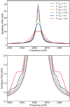 |
Fig. 1 Top: Effects of the convolution by the Fourier transform of the observational window on an ideal Lorentzian mode profile (grey) in the case of continuous observations, with ΓTobs = 0.25 (red), 0.5 (dark blue), 0.75 (green), 1 (orange), 2 (light blue), and 5 (brown). Bottom: Same as top panel, but for the y-axis range [1, 2]. |
2.6 Mode visibilities
It is often useful to be able to define the mode-height ratio between close-frequency modes. This can be achieved by computing the mode visibility, Vℓ, which depends on the stellar limb darkening and links the mode surface amplitude to the disk-integrated mode amplitude.
 (15)
(15)
where Pℓ is the ℓth-order Legendre polynomial and w is a weighting function. Assuming energy equipartition at close frequencies, the height ratio can be computed as the visibility ratio Vℓ/V0. For some instruments, the dependence is more complex as the instrument response does not depend only on µ. Hence, the relations given by Eq. (15) cannot be directly used (for an example with GOLF, see García et al. 1999; Salabert et al. 2011b). The values for Vℓ/V0 used in apollinaire are given in Table 2.
m-height ratios rℓ,m.
Mode visibility ratios Vℓ/V0
2.7 Modelling the modes for time-series with observational gaps
The apollinaire package is designed to deal with time series with large temporal gaps and was used for this purpose in Breton et al. (2022). The effect of the presence of gaps in the observations is the convolution of the Fourier transform of the ideal time series by the Fourier transform of the observational window. One of the consequences of this convolution is that the hypothesis on the frequency-bin independence is no longer valid (e.g. Gabriel 1994). However, the form of the likelihood that takes this effect into account is computationally challenging and not well suited for an optimised implementation.
The historically considered solution is to ignore the independence loss (Appourchaux et al. 1998) and to consider the likelihood given in Eq. (2). To go further, the model can be corrected to take into account the side lobes generated by the window convolution in the PSD (e.g. Salabert et al. 2002, Salabert et al. 2004). We use such an approach in apollinaire to modify the model when fitting PSD from time series with low duty cycle. In order to approximate the power redistribution of one peak in the model, we define the observation window ƒ of the time series. The value of ƒ is 1 at the time-stamps where data were acquired, and 0 otherwise. The Fourier transform
 of ƒ is then computed. The frequency shift vi (relative to the zero-frequency peak of
 ) and the amplitudes ai of the k peaks above a given threshold in
 are then stored. The amplitudes are normalised to verify
 (16)
(16)
The mode description given in Eq. (14) is then replaced by:
 (17)
(17)
The side lobe power redistribution of the mode is illustrated in Fig. 2, where we consider an observational window with a regular observation cycle of 720 min with observations followed by 720 minutes without observations. We consider a ℓ = 1,3 pair with i = 90° and vs = 0.4 µHz and we represent the model with 100% duty cycle for comparison. The power redistribution of the modes appears clearly when the formula from Eq. (17) is applied to compute the mode profiles, and we see that the modified model – approximating
 as the sum of k + 1 Dirac functions – is extremely close to the profile we obtain when we actually perform the convolution operation between the PSD and the |ƒ|2.
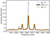 |
Fig. 2 Model for a ℓ = 1, 3 pair with inclination angle i = 90° and splittings s = 0.4 µHz, without taking the observational window into account (grey) and the modified model with the observational window effect applied following Eq. (17) (orange). The actual convolution of the synthetic PSD by |ƒ|2 is represented in black for comparison. |
3 Description of the framework
The apollinaire package is designed to perform MCMC samplings for each step of the peakbagging procedure: background fit, asymptotic parameters fit to determine the global modes pattern, and extraction of individual mode parameters. Those three operations are performed one after another when using the stellar_framework function but can also be performed independently. The global flowchart of an analysis performed with the stellar_framework function is represented in Fig. 3.
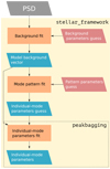 |
Fig. 3 Simplified representation of the apollinaire flow chart. |
3.1 Sampling the posterior probability with MCMC
The MCMCs are implemented with the Python package emcee (Foreman-Mackey et al. 2013). The sampling strategy follows Goodman & Weare (2010). The sampler, which can be seen as an improvement of the single site Metropolis scheme (Sokal 1997; Liu 2009), is designed as an affine invariant ensemble of walkers. Walker positions are updated one after another by the algorithm. The proposal for the new position of a given walker is created by taking into account the positions of other walkers. Acceptance or rejection of each move is assessed through the Metropolis-Hastings rule (Metropolis et al. 1953; Hastings 1970). In every part of the framework (background, global mode pattern, individual mode parameters), the user is free to choose the number of walkers and the number of steps to perform in order to sample the distribution, as well as the number of steps discarded as part of the burn-in phase.
The results yielded by a Bayesian approach strongly rely on the choice of prior functions made for the different parameters. At the same time, the prior function reflects the level of knowledge that the Bayesian fitters already possesses concerning the model for which they want to sample the posterior distribution. From this point of view, the choice of the prior functions to use in order to sample the posterior is necessarily somewhat arbitrary. Discussing considerations over the expected mode profile, several possibilities have been suggested in the Bayesian peakbagging literature. Following Benomar et al. (2012), Davies et al. (2016) considered for example a smoothness condition for the mode frequencies while using uniform priors for every other parameters. On the contrary, Lund et al. (2017) considered uniform priors for frequencies and inclination angle while using modified Jeffrey’s priors (Handberg & Campante 2011) for amplitudes and widths. Corsaro et al. (2020) adopted uniform priors for all free parameters, justifying this choice by the fast computation that it allowed in their framework.
In apollinaire, prior functions are taken to be uniform distributions within two bounds with the exception of the inclination angle, i, the heights H (or amplitudes A), and the widths Γ. It should be underlined that the uniform priors confine the sampled distribution to the compact support defined by the bounds and represent in this sense a strong constraint on the posterior. However, this can be justified by the fact that it is for example reasonable to suppose that, for a given mode, the actual mode frequency cannot be located outside a small frequency window around the mode power excess.
Most of the usual priors defined on a compact support can actually be linked to a uniform prior through a change of variable. For H (or A) and Γ, we therefore consider uniform prior distributions in log H (or log A) and log Γ. This is equivalent to constraining H (or A) and Γ with Jeffrey’s priors. This way, in the limit of the fixed boundaries, the prior does not contain information on the parameter scaling. For i, the prior distribution is p(i) = sin i in order to fulfill the a priori isotropic distribution of stellar rotation axes (García & Ballot 2019).
In the stellar_framework function, the automatically generated priors have been set in order to cover a sufficiently wide range to ensure that the sampled distribution is not biased by boundary effects. Additional difficulties that may arise in the specific case of frequencies are discussed in Sect. 3.5.
When a MCMC is sampled, the code automatically extracts summary statistics from it. For a given parameter, it returns the median of the marginalised sampled distribution, y. In order to obtain the uncertainties σ− and σ+ over y, 16th and 84th percentiles y16 and y84 are also extracted. In the case of a Gaussian distribution, σ− = σ+ = σ with σ being the standard deviation of the distribution. Some apollinaire output files (see Appendix D and online documentation for more details) only provide a σsym over y:
 (18)
(18)
In this case, if it is the natural logarithm of the parameters that has been sampled, median, 16th, and 84th percentiles are transformed again before computing and returning σsym.
3.2 Inputs and outputs
The guess and priors for background and global pattern fits are automatically generated by apollinaire. The user can also manually provide guess and priors if needed. The inputs for individual mode-parameter extractions are more complex, and for them, apollinaire uses text files with a specific syntax: the a2z files, which were originally developed as part of the A2Z pipeline (Mathur et al. 2010). The syntax of the file is dedicated to providing a simple and straightforward way to specify the nature, extent, initial value, and bounds for each parameter to fit. These files will be auto-generated by the stellar_framework function but can also be manually created in order to directly use the peakbagging function. They can be read as a pandas3 DataFrame through the auxiliary function read_a2z.
The chains are stored as Hierarchical Data Format version 5 (hdf5) files. The code provides functions to read these files for the user that would need to perform a more thorough analysis on the chains than the extraction of summary statistics described in Sect. 3.1. Using these files, it is for example straightforward to obtain the marginalised distribution for each parameter or the covariance matrix between two parameters. Corner plots visually summarising the sampled distributions can be saved as pdf or png files if filenames are specified. They represent both the marginalised distribution for each parameter and the covariance distribution for each pair of parameters.
Parameters fitted by the perform_mle_ background, perform_mle_pattern, explore_ distribution_background, and explore_distribution_ pattern functions are returned as numpy arrays. When these functions are called by the stellar_framework functions, the results they provide are stored in text files with dedicated headers. For convenience, the peakbagging function returns both an a2z DataFrame, which can be saved to an a2z file with the auxiliary function save_a2z, and a so-called pkb4 array, which can be saved with the save_a2z (when the function is called by stellar_framework, this is done automatically). The returned a2z DataFrame is useful for performing new MCMC samplings with modified input values while the pkb array provides a mode-by-mode summary statistics and allows the user to simply reconstruct the best-fit p-mode model computed by apollinaire. More details about a2z files, a2z DataFrame, pkb files, and pkb arrays can be found in Appendix D, and example a2z and pkb files are also provided.
3.3 Background fit
Besides the PSD, the only additional inputs needed by apollinaire to automatically compute initial guesses and priors for the background fit are the stellar effective temperature, Teff, the asymptotic large spacing Δν, and the frequency at maximum power vmax. If no previous estimations of Δν and vmax are available, it is possible to provide the code with the stellar mass, M, and radius, R, in order to compute an estimate of Δν and vmax through the scaling laws (Kjeldsen & Bedding 1995)
 (19)
(19)
where Δν⊙, M⊙, R⊙, and Teff,⊙ are the reference solar values for the asymptotic large spacing, mass, radius, and effective temperature, respectively. These values are set to 135 µHz, 1 M⊙, 1 R⊙, and 5770K in apollinaire.
The limit spectrum fitted on the data is the sum of the background term given by Eq. (6) and a Gaussian p-mode envelope term:
![Mathematical equation: ${I_1} = \left[ {{v_{{k_0}}},{2 \over 3}{v_{\max }}} \right],$](/articles/aa/full_html/2022/07/aa43330-22/aa43330-22-eq35.png) (20)
(20)
with Hmax being the maximal height of the p-mode Gaussian envelope and Wgauss its width or standard deviation.
When only one Harvey model is considered, the initial γ value is fixed to 2; it is fixed to 4 when two Harvey models are considered. This parameter can be fixed (Kallinger et al. 2014) or set to vary. In order to fit more than two Harvey models, the user should manually provide the guesses. Otherwise, input profile guesses are automatically generated. If the spectrum has been acquired with photometric observations, the values provided by Table 2 of Kallinger et al. (2014) are used. If the code has to deal with a PSD obtained from a solar radial-velocity time series, initial guess values have also been implemented using GOLF as a reference.
In order to obtain significant gains in computing time, it is possible to resample the PSD to a version with many fewer data points. The resampling techniques are described in Appendix A. As shown in Sect. 4.3, this method can be reliably used in order to extract mode frequencies but the main caveat is that the background parameters obtained by fitting the resampled PSD should be considered with caution. In particular, the resampling will filter out the power in the p-mode region, and Hmax, vmax, and Wenv obtained with this method will be significantly biased.
3.4 Limit p-mode spectrum
To fit the p modes, apollinaire divides the observed spectrum by the fitted background profile B in order to get the signal-to-noise-ratio (S/N) spectrum:
![Mathematical equation: ${I_2} = \left[ {{2 \over 3}{v_{\max }},{3 \over 2}{v_{\max }}} \right],$](/articles/aa/full_html/2022/07/aa43330-22/aa43330-22-eq36.png) (21)
(21)
This way, the background contribution fitted in the previous step is removed. The limit spectrum, SSN, that is then adjusted to Sobs,SN is
![Mathematical equation: ${I_3} = \left[ {{3 \over 2}{v_{\max }},{v_{{\rm{Nyquist}}}}} \right].$](/articles/aa/full_html/2022/07/aa43330-22/aa43330-22-eq37.png) (21)
(21)
with Mn,ℓ given by Eq. (14), and b corresponding to an additive factor to locally adjust the background.
3.5 Pattern fit
In order to constrain the priors of the main individual mode parameters, vn,ℓ, Hn,ℓ, and Γn,ℓ, apollinaire performs a global pattern fit on the orders located around vmax. Tassoul (1980) presented the following asymptotic relation for mode frequencies, within the approximation n » ℓ:
 (23)
(23)
where ϵ is a phase constant. Slightly modifying the formalism adopted in Lund et al. (2017), this relation can be approximated, in the vmax neighbourhood, to
 (24)
(24)
where the small separations δν0ℓ are given by
 (25)
(25)
while α and β0ℓ are respectively the curvature terms on Δν and δν0ℓ. The parameter nmax, which is not an integer, follows the relation
 (26)
(26)
Mode heights in the limit spectrum can be approximated through the p-mode envelope parameters Hmax and Wgauss, considering
 (27)
(27)
while Γ is taken as a FWHM value common to all modes.
Using Eqs. (24) and (27), the pattern fit step is designed to approximate the mode pattern around vmax with a given set θ of global parameters: ϵ, α, Δν, vmax, Hmax, Wgauss, Γ, δν02, β02, δν01, β01, and δν13 (with δν13 = δν03 − δν01), β03. The last four parameters can be ignored, for example if the star to fit presents ℓ = 1 mixed modes: only pairs Mn−1,2, Mn,0 will then be fitted (see Appendix B). It is also possible to ignore just the ℓ = 3 mode when the S/N of the considered PSD is insufficient. Indeed, in this situation, the δν13 and β03 parameters will be difficult to constrain and the sampled distribution will be prior dominated.
Guesses for ϵ, α, Hmax, Γ, δν02, δν01, and δν13 can be manually provided, otherwise they will be automatically computed. If a guess is given for a δν0k, the initial value for the corresponding β0k will be set to zero. To determine initial automated guesses for parameters, we adopted prescriptions from Corsaro et al. (2012) for stars with Δν < 14 µHz and vmax < 450 µHz. For main sequence stars, we derived well performing initial values from the results obtained by Lund et al. (2017). Proper guesses for stars with 450 µHz < vmax < 1000 µHz are not implemented in the current version of apollinaire but a recipe for how to proceed with these stars is given in Appendix B.
The pattern fit step will fit θ by considering the k orders closest to vmax. By default, the stellar_framework function uses k = 3. The bounds of the fitting window are set 0.2 Δν below and above the smallest and largest mode frequency included in the pattern. In the standard procedure, the MCMC exploration is directly performed from the initial rough guess computed by apollinaire. It is possible to use a fast MLE run to quickly refine this initial guess and to use the values yielded by the MLE as a starting point for the MCMC sampling. This can save some computing time by reducing the number of discarded steps at the beginning of the MCMC exploration, but may also reduce the opportunities of the walkers to explore different regions of the distribution to sample in the case of multimodal distribution.
As underlined by Lund et al. (2017), the discrepancies between the actual position of the modes and the frequencies yielded by the relation given by Eq. (24) can be physically explained by acoustic glitches (e.g. Mazumdar et al. 2014; Houdayer et al. 2021). Moreover, when optimised only on the central orders, the formula given by Eq. (24) should be extrapolated with caution for modes located far from vmax Indeed, in this case, there can be significant discrepancies between the mode frequencies predicted by the formula and the actual position of the mode in the PSD. This can be straightforwardly checked using an échelle diagram and is illustrated in particular in Sect. 4.3. It is of course possible to include more orders when sampling the distribution of pattern parameters, but this will require more computing time; on one hand because the likelihood will be computed on more data points, and on the other because the chain will take more steps to converge. In this situation, the results obtained with the summary statistics alone should also be considered with caution as the inclusion of low-S/N modes can strongly influence the multi-modality of the sampled distribution.
An échelle diagram may also be particularly useful in order to check that the code correctly identified the ℓ = 0 and the ℓ = 1 mode. When this is not the case, the failure in the sampling is generally related to an improper prior for ϵ. In this situation, the solution is to manually impose new initial values and prior bounds for ϵ.
3.6 Selecting orders to fit
The result of the pattern fit is used to obtain guess values for νn,ℓ Hn,ℓ, and Γn,ℓ for each mode. These values are provided inside an a2z DataFrame. There are two ways to determine the modes for which the function will provide guess values. With the first method, the function will simply build the a2z DataFrame for a given number of orders symmetrically distributed around vmax The second method performs a H0 screening (e.g. Appourchaux et al. 2009, 2012; Broomhall et al. 2010; Davies et al. 2016; Lund et al. 2017) on the p-mode region to assess the strong (ℓ = 0 or 1) mode detectability. Following the procedure presented in Davies et al. (2016), the PSD is rebinned over t bins and
 statistics is considered. For each mode, the rebinning is performed considering an odd number of bins, the central bin being the one with the frequency closest to the mode frequency estimated with the fitted global parameters. The adopted threshold for the rejection of the null hypothesis H0 is p = 0.001. The maximal value tmax considered for the rebinning is 99, or the t value corresponding to a bin width of 5 µHz, respectively. If the H0 hypothesis is rejected for more than one-third of the considered rebinning, we consider the mode as detectable. A guess for this mode will be added in the a2z DataFrame along with the guess for the closest ℓ = {2, 3} mode. It should be stated that it is also possible to manually provide a a2z DataFrame that will override the guess automatically generated by the function.
3.7 Extraction of individual parameters: the peakbagging function
In what follows, we refer to the Mn−1,2, Mn,0, Mn−1,3, and Mn,1 group of modes as a peakbagging order to avoid any confusion. Mode parameters can be fitted globally, by peakbagging order, or by pair. In the latter case, modes Mn−1,2, Mn,0, or Mn−1,3 ,and Mn,1 are then fitted together, respectively. The reader should note that the pair-fitting strategy is also suited to fitting any individual mode if the parameters of only one mode of a given pair is specified in the a2z input. The model used to compute the likelihood and posterior probability follows Eq. (22). The initial value for the local S/N background term b is taken as 1 and set to vary between 10−6 and 5.
The minimal set of parameters that will be fitted by the code are mode frequencies, νn,ℓ, heights, Hn,ℓ (or amplitudes, An,ℓ), and FWHM, Γn,ℓ. Additional parameters that can be fitted are splittings, sn,ℓ, inclination angle, i, and asymmetries, αn,ℓ. It is possible to fit the projected splittings, s✶ = s sin i (Ballot et al. 2006, 2008), instead of s. Except for mode frequencies, every input parameter can be set to parametrise all modes, a whole order, a pair, or only one mode. In other words, it is possible to impose each mode of a given peakbagging order to have, for example, the same FWHM.
If the user does not provide a fitting window size, the data to fit are restricted to an adaptive fitting window: only PSD elements within [ν−, ν+] are considered, with:
 (28)
(28)
where vlow and vup are respectively the minimal and maximal guess frequencies of the modes to fit. The value of d is then determined by the considered method: if the fit is made by order, d = 3, if the fit is made by pair, d = 1.
For modes above 800 µHz and if the fit is made by pair, another possibility offered by the code is to use the Δν value to constrain the fitting window. The 800 µHz value has been chosen to ensure that the considered mode does not exhibit avoided crossings, which might add additional difficulties due to the potential presence of mixed modes in the fitting window. In this case, the window bounds are:
 (29)
(29)
where vcenter is the centre of the window given by the mean of the guess frequencies of the two modes to fit (or simply the guess frequency of the mode to fit if only parameters for one mode are specified), and the reference value Δν⊙ = 135 µHz. The possible values of ww are summarised in Table 3.
As underlined in Sect. 2, the mode visibilities and m-height ratios have instrumental dependencies. There are two ways to deal with mode visibilities: on one hand, the user can choose to fit amplitude parameters individually for each mode, and on the other, it is possible to specify the amplitude ratios Vℓ/V0 in the a2z input file. The usual ratios (Salabert et al. 2011a) are provided in Table 2.
The m-height ratios to use are selected through the instrument argument of the peakbagging function. The implemented ratios for each instrument are given in Table 1.
It should also be noted that for H and Γ, it is the natural logarithms of the parameters that are expected to have a Gaussian distribution (Toutain & Appourchaux 1994; García & Ballot 2019). For parameters of these types, the peakbagging function thus samples the natural logarithm. However, it should be remembered that it is straightforward to obtain the sampled distribution of the parameter itself by a simple transformation of the MCMC elements.
Possible values of ww.
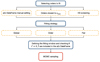 |
Fig. 4 Summary of the available options for the p-mode individual parameter extraction step. |
3.8 Dealing with ℓ = 4 and ℓ = 5 leaks in solar spectra
Due to the very high S/N of radial-velocity helioseismic data, some ℓ = 4 and ℓ = 5 modes (referred as intermediate-degree modes) may arise above noise. It has been shown that omitting their contribution to the power distribution of the spectrum can introduce bias in the fitted frequencies of up to three times the uncertainty (Jiménez-Reyes et al. 2008). If guesses for intermediate-degree modes are specified in the input a2z file (e.g. using the theoretical frequency value for those modes), the code will check for their presence inside the defined window.
If, when reading the a2z DataFrame, it appears that an intermediate-degree mode is present in the fitting window, its frequency will be added to the parameters to fit. Heights and FWHMs of intermediate-degree mode are computed considering the ratio presented in Table 2 and using the closest ℓ = 0 mode as a reference. If no ℓ = 0 is fitted at this time, the closest ℓ = 1 is used instead. Power is distributed between the m-components of the mode following Table 1. The splittings are set to 400 nHz and do not vary. No asymmetry is considered for these modes. The diagram shown in Fig. 4 summarises the possible options described in Sects. 3.6, 3.7 and 3.8.
3.9 Quality assurance
Several frequentist and Bayesian metrics for peakbagging quality assurance have been suggested over the years (see e.g. Appourchaux et al. 2012; Davies et al. 2016; Lund et al. 2017). The quality assurance metric implemented in apollinaire takes inspiration from the Bayesian machinery described in Davies et al. (2016) but avoids resampling a MCMC to obtain the probability of the different models to compare, which saves a large amount of computing time.
The apollinaire package implements a Bayesian quality assurance computing tool where three possibilities are assumed for each fitted pair of modes (odd or even): (1) The strong (ℓ = 0 or 1) and the weak (ℓ = 2 or 3) modes are both detected (model Msw with associated probability psw); (2) only the strong mode is detected (model Ms with associated probability ps); or (3) neither of the two modes is detected (model M0 with associated probability p0). We have assumed that a weak mode could not be detected if the strong mode was not also detected. Assuming that a sufficient number of initial steps has been discarded, the MCMC contains n sets of parameters θ. A subset of k (k ≤ n) elements still representative of the MCMC distribution can be selected by thinning the chain. Indeed, this subgroup of parameters should follow the same distribution as the full MCMC if enough elements are considered. For each of those k sets of parameters θk, likelihoods p(D|Msw, θk), p(D|Ms, θk), p(D|M0, θk) corresponding to the three hypothesises are then compared (considering the data D within the same frequency window that was used for the actual fit). For the M0 model, as the frequency window is narrow enough, we consider a flat background which is computed as the median of the power distribution of the frequency bins inside the window.
The estimated probability pα (marginalised over the parameter distribution) that a model Mα is the most likely considering the data is then computed as follows:
 (30)
(30)
where given an ensemble E, #E denotes its cardinal. The indexes α, β and γ in Eq. (30) should be properly replaced by sw, s, and 0 depending on the considered case. We use Eq. (30) to estimate the probability pα as the fraction of explored parameter sets θk for which the model α is the most likely among the three models. If we consider the specific case where n = k, Eq. (30) gives the exact proportion of cases in the sampled distribution where the Mα model is the most likely. The probability pα is therefore the likelihood of Mα for this distribution. The thinning step to reduce to k samples allows a significant gain in computing time to obtain pα while conserving the sampled distribution properties.
p0 is the probability of the null hypothesis H0 for the detection of the strong mode while ps + p0 is the H0 probability for the weak mode. For the considered pair, the natural logarithm of the Bayes factor K for the detection of a mode of degree ℓ is then given by:
 (31)
(31)
Here we reiterate the interpretation of the ln K value for the evidence against H0, as outlined by Kass & Raftery (1995) :

It is easy to see that, if the model psw, for example, is favoured in any case, this will correspond to psw = 1 and therefore ln K > 5. If we have psw = 2/3 and p0 = 1/3, we will have ln K ≈ 0.69, and the Msw model is only barely favoured compared to the H0 hypothesis. Modes with ln K < 1 should be cautiously considered when exploiting the peakbagging results for modelling purposes.
4 Benchmark with Monte Carlo synthetic spectra and published peakbagging results
In this section, in order to assess the reliability of the code, we present the results of a Monte Carlo benchmark with synthetic spectra. We then compare apollinaire results with results obtained with other peakbagging codes. As the method has been designed to perform helioseismic and asteroseismic analysis, we decided to perform our benchmark with both solar and stellar data5.
Mode parameters of the three pairs used for the Monte Carlo trial.
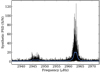 |
Fig. 5 Example of a synthetic spectrum generated with the pair 2 set of parameters and a frequency vector with 1460-day resolution (black). The ideal spectrum is overplotted in blue. |
4.1 Monte Carlo trial
Considering three different sets of parameters (see Table 4), we generate a limit spectrum for three pairs of modes. This limit spectrum is then multiplied by a noise vector with a power distribution following a χ2 with two degrees of freedom. The pairs are generated for two frequency vectors: the first with one-year resolution and the second with four-year resolution. An example of such a synthetic pair is shown in Fig. 5. Each pair is then fitted using the peakbagging function. For each pair and each resolution, we repeat this process 200 times. For each considered pair and resolution, Tables 5 and 6 summarise the percentage of times for which the true value, considering the uncertainties, is outside the 68% and 99.7% credible intervals, defined by the 1σ and 3σ departure from the fitted value, respectively, with the fitted value taken as the median of the sampled distribution. The percentage of fits for which we find the true value to be in the 68% and 99.7% credible intervals is therefore close to expectations, the standard deviation for the frequency of success being 3.3% in the case of 200 draws following a binomial law of parameters (ndraw = 200, p = 0.68), and 0.4% for (ndraw = 200, p = 0.997), with ndraw being the number of draws.
When we consider the 2400 fitted frequencies at once, we find the uncertainties obtained with apollinaire to be conservative in this experiment. Indeed, 71.5% of the fitted frequencies are in the 68% credible interval. With a standard deviation of 0.95% for 2400 independent experiments, this is approximately four standard deviations away from the 68% expected value.
We note that the uncertainties obtained for the 1460-day pairs are significantly smaller than for the 365-day pairs. An example comparison between the true value and apollinaire fitted value is shown in Figs. 6 and 7, where the frequency error νfitted – νtrue between the fitted value and the true value is represented for the ℓ = 1 mode of pair 2. The spread reduction of the error distribution appears clearly in the histograms. Figure 7 also shows the (νfitted – νtrue) /σ distribution where we specify the mean value 〈(νfitted – νtrue) /σ〉. As expected, the standard deviation for the (νfitted – νtrue) /σ distribution is close to 1 in both cases. We find no systematic bias in the fitted parameters, except for the splittings in pair 3 which are systematically underestimated due to the large mode width.
Percentage of values in the 68% and 99.7% credible intervals for the strong (ℓ = 0,1) mode in the Monte Carlo trial.
Percentage of values in the 68% and 99.7% credible intervals for the weak (ℓ = 2, 3) mode in the Monte Carlo trial.
4.2 GOLF solar PSD analysis
To study the p-mode frequency shifts induced by the magnetic solar cycle, Salabert et al. (2015) performed an analysis of 69 one-year subseries of the GOLF instrument, spanning from 1996 April 11 to 2014 March 5, with 91.25 days overlap. The modes were fitted using a MLE method (Salabert et al. 2007). In order to compare the results from this method with apollinaire fits, we use the same MLE code to perform a similar analysis by considering subseries of 1-yr spanning from 1996 April 11 to 2020 July 6, with a 91.25 days overlap6. We remove five subseries that have a duty-cycle of below 90% and therefore consider 89 subseries. For each of these subseries, we fit modes ℓ = 0, 1, 2, 3. However, as ℓ = 3 have low signal-to-noise ratios in the GOLF data, we compare only the results obtained for mode ℓ = 0, 1, 2 in the following. The lowest frequency considered mode is n = 11, ℓ = 2 while the highest frequency considered mode is n = 26, ℓ = 1. This means that we compare fit results between apollinaire and the MLE method for 4005 modes. The procedure to fit the series with apollinaire is the following. Frequency bins below 50 µHz are not considered to fit the background. The S/N spectrum is then computed by dividing the PSD by the fitted background model. Modes are fitted by pair. Heights Hn,ℓ, FWHMs Γn,ℓ and splittings sn,ℓ are fitted independently for each mode. As asymmetries are expected to depend on frequency only, one asymmetry value is fitted for each pair. Finally, ℓ = {4, 5} power leakages are accounted for during the fit. For the background fit, the MCMC are sampled with 500 walkers iterated over 500 steps, with the 100 first steps discarded as burn-in. For the individual mode fit, the MCMC are sampled using 500 walkers iterated over 1000 steps. The 400 first steps are discarded to take the burn-in phase into account.
We consider the 1σ and 3σ intervals relative to the values and corresponding uncertainties σ fitted with apollinaire. Among the 4005 fitted modes, the frequencies fitted by the MLE method, vmle, lay outside the 1σ interval for 38 modes (0.9%) and outside the 3σ interval for 10 modes (0.2%). The MLE heights Η lay outside the 1σ interval for 464 modes (11.5%) and outside the 3σ interval for 23 modes (0.6%). The MLE FWHMs Γ lay outside the 1σ interval for 185 modes (4.6%) and outside the 3σ interval for 18 modes (0.4%). The relatively high number of Η and Γ values laying outside the 1σ interval can be explained by the strong anti-correlation that exists between these two parameters, especially at high frequency. We also identify at least two modes that have not been correctly fitted by the MLE method. Finally, we represent the
 distribution in Fig. 8 in order to show the comparison of the two methods exhibits no systematic bias.
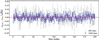 |
Fig. 6 Error νfitted – νtrue /σ on the ℓ = 1 mode from pair 2 and corresponding uncertainties for every Monte Carlo run with 365-day (grey) and 1460-day (blue) resolution. The zero vertical coordinate is highlighted by the red dashed line. |
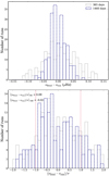 |
Fig. 7 Top: νfitted – νtrue distribution on the ℓ = 1 mode from pair 2 for every Monte Carlo run with 365-day (grey) and 1460-day (blue) resolution. Bottom: (νfitted – νtrue)/σ distribution on the ℓ = 1 mode from pair 2 for every Monte Carlo run with 365-day (grey) and 1460-day (blue) resolution. The mean value 〈(νfitted – νtrue)/σ〉 for both distributions is specified and the standard deviation of the 1460-day distribution is shown in red. |
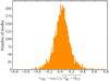 |
Fig. 8
|

4.3 The Kepler main sequence LEGACY catalogue
In order to extract strong modelling constraints to be used in stellar evolution codes Silva Aguirre et al. (2017), hereafter L 17, performed a thorough peakbagging analysis of the so-called Kepler LEGACY sample, which contains 66 main sequence stars with stochastically excited ρ modes7. We select six targets to analyse within the LEGACY sample, namely KIC 5184732, 6106415, 6225718, 6603624, 12069424, and 12069449, and we compare the apollinaire results to the reference values provided by L 17. Some fundamental stellar properties of the selected targets are given in Table 7, which are taken from the Kepler data release 25 (DR25, Mathur et al. 2017).
As we want to show how apollinaire behaves when used blindly without any previous knowledge of the seismic values, effective temperatures Teff, masses M, and radii R are used to estimate vmax and ∆v values from the global seismic scaling laws. We could also have used the vmax and ∆v values from L17 as input. The PSDs we analyse were obtained from KEPSEISMIC-calibrated8 light curves (García et al. 2011). The background profile is fitted considering two Harvey models and a flat noise contribution (see Sect. 2.2). We fit the background with the complete PSD, but in order to assess the effect of a background fit performed on a rebinned PSD on the mode frequencies, we also sample the posterior probability of our background model on a PSD resampled following the method described in Appendix A. Frequency bins below 50 µHz are not considered. We use 500 walkers iterated over 5000 steps, with the 100 first iterations discarded as burn-in. We deliberately choose a large number of steps to ensure the convergence of the chains. The global mode pattern is adjusted on the S/N spectrum obtained by dividing the PSD by the background model, according to the strategy described in Sect. 3.5 and considering ℓ = {0, 1, 2, 3} of the three orders closest to vmax. We use 500 walkers iterated over 5000 steps and we discard the 250 first drawn points. We visually check that the fitted pattern has a satisfying profile in order to provide correct frequency guesses for the individual mode-parameter extraction. In the individual mode parameter fit, for each target, we limit our analysis to the seven orders closest to vmax. All the chosen targets have a p-mode S/N that is sufficient to fit mode parameters farther from vmax, but we make this choice in order to ensure that the frequency estimates yielded by Eq. (24) are correct and to avoid a manual redefinition of the priors for low- and high-order modes before sampling the mode parameters. The MCMCs are sampled using 500 walkers iterated over 5000 steps. The 200 first steps are discarded to take the burn-in phase into account.
For each fitted parameter, L17 specified two uncertainty values (in the same way apollinaire allows computing σ+ and σ−). For sake of simplicity and clarity in the comparison of results, we consider only the larger uncertainty value for each parameter. L17 epsilon ϵ values are compared to the results yielded by apollinaire in Fig. 9. The echelle diagrams obtained from the apollinaire fits are provided in Fig. 10 where we also represent the frequencies obtained from Eq. (24) and the corresponding pattern sampling. As already underlined in Sect. 3.5, the echelle diagram clearly shows that, as we constrained the parameters from Eq. (24) on only the three central orders, the predicted value we obtain for modes far from vmax does not follow the actual node ridge in the échelle diagrams. Fitted frequencies are compared with the values from L17 in Fig. 11. The same type of comparison is performed for mode amplitudes and FWHMs in Fig. 12. The apollinaire fitted values and reference from L17 can be found in Tables 8, D.3, and D.4, along with the quality assurance values In K computed according to the method presented in Sect. 3.9. The results are globally in agreement for frequencies. Considering the 1σ and 3σ interval relative to the apollinaire value again over the 154 fitted frequencies, the L17 frequency is beyond 1σ for 39 modes and beyond 3σ for three modes. We find larger discrepancies for mode amplitudes and widths: over the 42 fitted widths (one per order), the L17 value is outside the 1σ interval 25 times and outside the 3σ interval 8 times. Over the 42 fitted amplitudes, the L17 value is outside the 1σ interval 31 times and outside the 3σ interval 12 times. We find no systematic bias in the frequency, amplitude, and width comparison. Concerning the mode frequencies, the largest observed discrepancy between L17 and apollinaire is found to be on the KIC 006603624 mode M18,3. We have v18,3,apn = 2299.52 ± 0.20 µHz and v18,3,L17 = 2305.47 ± 0.13 µHz. However, inspecting the KIC 006603624 spectrum and the corresponding echelle diagram, it seems more credible to us that the correct position of this mode is the one yielded by apollinaire.
The discrepancies in the values obtained for fitted parameters can have multiple explanations. While we used KEPSEISMIC data, L17 exploited light curves corrected with the KASOC filter (Handberg & Lund 2014). The data calibration influences the power redistribution in the PSD frequency bins and may therefore be responsible for some of the observed discrepancies between the mode widths and amplitudes, and, to a lesser extent, for frequency discrepancies. However, when comparing peakbagging codes, it is found that the main discrepancies are induced by the differences in the methods used to fit the background (Appourchaux et al. 2014). It should also be underlined that there are several differences in the models we use when compared to those used by L17. The first main difference resides in the fact that L17 included the Vℓ parameters for which posterior probability distributions are sampled while these parameters were fixed in our model (see Sect. 2.6). The second difference is that, as we fit order by order, the inclination angle i is poorly constrained with this choice of strategy. It is also important to keep in mind that the uncertainty values yielded by a MCMC process are only formal uncertainties related to the variance of the parameters inside a given model confronted to the data. It has already been demonstrated that an inaccurate description (e.g. by neglecting the ℓ = 4, 5 contribution or the wing power of the modes outside the fitting window) of the mode profiles could bias the estimation of the real values by several times the uncertainty values (Jiménez-Reyes et al. 2008).
Concerning ϵ values, L17 and White et al. (2011) noted that a strong anti-correlation exists between Δν and ϵ. We also note that for most vmax Δν, and ϵ, the apollinaire uncertainty values are much larger than for the L17 values. For KIC 006225718, for example, apollinaire yielded Δν = 106.78 ± 0.43 µHz while L17 gave Δν = 105.695 ± 0.018 µHz. This can be explained by the fact that, even if our Eq. (24) is really close to Eq. (27) of L17, the strategy exploited to sample the parameter distribution is totally different. We use Eq. (24) together with Eq. (27) and a common Γ value in order to compute a mode profile for the three central orders and directly constrain our parameters with the PSD. On the contrary, L17 used their Eq. (27) to constrain the pattern parameters from the individual mode frequencies they had already obtained from the PSD analysis.
Finally, Fig. 13 shows the  distribution, where νfull and σfull are the frequencies and uncertainties obtained by considering the complete PSD for the background fit, and vresampled and σresampled are the frequencies and uncertainties obtained after using the background fitted on the resampled PSD. This shows that, for mode frequencies, the discrepancies between the two methods are negligible with respect to the fitted uncertainties, which means that frequencies obtained with the PSD resampling method can be used without risk as input for modelling codes. This resampling strategy is made relevant in the optic of the PLATO mission preparation, where it will be necessary to perform the peakbagging analysis for tens of thousands of stars in an optimised computing time.
KIC and fundamental stellar properties of selected targets from the LEGACY sample.
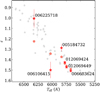 |
Fig. 9 L17 ϵ values (pentagons) compared to apollinaire ϵ values (stars) for the six considered targets. Corresponding KIC are specified next to each red dot. The epsilon values obtained by L17 for the other stars of the LEGACY sample are represented in grey. Some of the uncertainties are too small to be represented on the figure. |
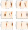 |
Fig. 10 Échelle diagram of the six selected targets apollinaire fitted p-mode frequencies (black diamonds) with corresponding error bars. The blue circles signal the frequency initial guesses inferred from Eq. (24). |
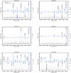 |
Fig. 11 Comparison of p-mode frequencies yielded by apollinaire (dark blue) and reference values from L17 (light blue). The error bars overlapping intervals are represented in medium blue. The KEPSEISMIC PSD are represented in light grey while the apollinaire fitted model is shown in dark grey. |
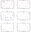 |
Fig. 12 Comparison of p-mode FWHMs and amplitudes yielded by apollinaire (dark blue and red, respectively) and reference values from L17 (light blue and salmon, respectively). The error bars overlapping intervals are represented in medium blue and dark salmon, respectively. |
Comparison between vmax, Δν, and ϵ values yielded by apollinaire and reference values from L17.
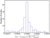 |
Fig. 13
|

5 Discussion
The possibilities offered by MCMC sampling methods and the flexibility of the possible strategies allowed by apollinaire merit a brief discussion. Another question that arises when using MCMC is the hyper-parameters value that must be chosen in order to correctly dimension the problem. We decided in this paper to use 500 walkers for all the sampling we perform, which is a typical value used in several peakbagging studies (see e.g. Davies et al. 2016; Lund et al. 2017). Choosing the optimal number of steps to perform when sampling the chain and the proportion of steps that should be burned in at the beginning of the run represents a complex issue that has no universal solution. This can only be done through test and trial, especially when the initial guesses appear to be quite far from the posterior probability optimum. One way to check that the chain is fully converged is to split it in half after having removed the burned in elements and to verify that the shapes of the two subdistributions are identical. It is also possible to estimate the auto-correlation time τ of the chain to assess its convergence. However, obtaining a reliable estimate of τ requires running the sampling for at least 50τ steps, which can prove extremely computationally extensive. Having run a sampling experiment with KIC 6603624 as reference, we find that, when the posterior is data dominated, τ values are typically of a few hundred steps. Parameters for which the posterior is prior dominated typically have longer auto-correlation times.
It is also important to keep in mind that some fitting strategies may have to be preferred considering the target being analysed. For example, for high-resolution solar data, we will favour a fit by pair, with the height and the FWHM of each mode set to vary freely. Mode asymmetries should be fitted for modes above 2450 µHz. In stellar data, especially with low-resolution low-S/N data, modes will be fitted globally or by order, with a constraint on the mode-relative amplitudes. It will only be possible to constrain the stellar inclination angle where good S/N data are available; in this case, it will be necessary to perform a global fit in order to consider the m-height ratio of the largest possible number of modes at the same time. Mode asymmetries are usually not considered when fitting stellar data. The user may keep in mind that when fitting all the modes at once with a global method, the MCMC will converge more slowly because of the increased number of dimensions in the parameter space being explored. For power spectra obtained from short time series, because of the mode stochastic excitation, allowing the mode FWHM and height to vary freely may sometimes yield better results than using the ratios specified in Table 2.
6 Conclusion
In this paper, we introduced the apollinaire module, an open-source Python 3 package designed for helio- and asteroseismic disk-integrated peakbagging. The module implements a set of functions that are able to extract background, p-mode global pattern, and p-mode individual parameters through MCMC sampling implemented with emcee. The implementation of these functions is designed to provide a flexible framework. They can be used independently or combined depending on the task the user wants to achieve.
We analysed data from the GOLF instrument and the Kepler LEGACY sample in order to compare apollinaire results with values available in the literature. We find good agreement between our results and the reference values. The discrepancies can be explained by differences in data calibrations, fitting strategies, and adopted models.
The code is in active development and the online repository is regularly updated. An online documentation of the package is available and includes several tutorials that should allow any interested user to quickly start working with apollinaire and use the different functions to analyse their own set of data. With the increasing number of TESS targets of asteroseismic interest and the preparation of the PLATO mission, we hope that apollinaire will become a widely used tool in the community.
Acknowledgements
The authors thanks the anonymous referee for constructive comments and precious suggestions that greatly enriched and completed the material of the paper. S.N.B, and R.A.G acknowledge the support from PLATO and GOLF CNES grants. J.B. acknowledges the support from CNES. V.D. acknowledges the support of the IAC (Tenerife, Spain). The authors are deeply grateful to G.R. Davies who originally designed the a2z data structures in collaboration with R.A.G. They also thank L. Bugnet, M. Delorme, A. Jiménez, S. Mathur, and V. Prat for fruitful discussions. A special thank to A. Finley for his precious suggestions concerning the name of the paper. This paper includes data collected by the Kepler mission. Funding for the Kepler mission is provided by the NASA Science Mission Directorate. This research has made use of the VizieR catalogue access tool, CDS, Strasbourg, France (DOI : 10.26093/cds/vizier). The original description of the VizieR service was published in 2000, A&AS 143, 23. Software: Python (Van Rossum & Drake 2009), numpy (Oliphant 2006; Harris et al. 2020), pandas (Pandas development team 2020; Wes McKinney 2010), matplotlib (Hunter 2007), emcee (Foreman-Mackey et al. 2013), scipy (Virtanen et al. 2020), corner (Foreman-Mackey 2016), astropy (Astropy Collaboration 2013, 2018), h5py (Collette 2013), george (Ambikasaran et al. 2015). The previous references should be cited together with apollinaire when using the module. Packaged version of apollinaire can be installed through pip and conda-£orge (Conda-forge community 2015). The source code and most recent versions of apollinaire can be found at https://gitlab.com/sybreton/apollinaire while the module documentation is hosted at https://apollinaire.readthedocs.io/.
Appendix A PSD resampling for background fit
We included several resampling strategies in apollinaire in order to perform quicker background fits (the computing time of the MCMC process being mainly constrained by the length of the vector on which the posterior probability is computed at each step). We describe here the resampling methods implemented in the module. The user has the choice between two resampling strategies, reboxing and advanced_reboxing.
The reboxing strategy uses the numpy.logspace function to create a new frequency vector with logarithmic frequency spacing and a number of data points specified by the user. The logarithmic spacing is preferred over a linear spacing in order to increase the proportion of low-frequency data-point in the fit. Each bin of the original PSD is then attributed to a box considering the closest frequency bin in the new frequency vector. The median of each box is then considered in order to compute the resampled PSD.
In order to apply a distinct resampling to the p-mode region, the advanced_reboxing extends this approach with a more subtle resampling techniques. In this case, the user specifies a target number N of data points in the resampled PSD outside the vmax region and a number M of data points in the vmax region. Considering consecutive frequency bins vk and νk+1, they are directly put in the resampled frequency vector under the condition
 (A.1)
(A.1)
We define k0 as the frequency bin verifying:
 (A.2)
(A.2)
and three frequency intervals Ij· = [νa, vb] such as
![Mathematical equation: ${I_1} = \left[ {{v_{{k_0}}},{2 \over 3}{v_{\max }}} \right],$](/articles/aa/full_html/2022/07/aa43330-22/aa43330-22-eq55.png) (A.3)
(A.3)
![Mathematical equation: ${I_2} = \left[ {{2 \over 3}{v_{\max }},{3 \over 2}{v_{\max }}} \right],$](/articles/aa/full_html/2022/07/aa43330-22/aa43330-22-eq56.png) (A.4)
(A.4)
![Mathematical equation: ${I_3} = \left[ {{3 \over 2}{v_{\max }},{v_{{\rm{Nyquist}}}}} \right].$](/articles/aa/full_html/2022/07/aa43330-22/aa43330-22-eq57.png) (A.5)
(A.5)
For each frequency interval, the box size parameter Sj is
 (A.6)
(A.6)
with
 (A.7)
(A.7)
 (A.8)
(A.8)
 (A.9)
(A.9)
and the parameter C is given by
 (A.10)
The bounds of the consecutive boxes in the Ij interval are then
![Mathematical equation: $\left[ {{v_a},{S_j}{v_a}} \right],\,\,\left[ {{S_j}{v_a},S_j^2{v_a}} \right],\,\, \ldots ,\,\,\left[ {S_j^{{N_j} - 1}{v_a},{v_b}} \right]$](/articles/aa/full_html/2022/07/aa43330-22/aa43330-22-eq63.png) . Inside each box, the new PSD bin is taken as the median of the PSD values in the box while the corresponding new frequency bin is computed by considering the geometric means of the frequencies inside the box
. Inside each box, the new PSD bin is taken as the median of the PSD values in the box while the corresponding new frequency bin is computed by considering the geometric means of the frequencies inside the box
 (A.11)
with nbin the number of frequency bins inside the box.
Appendix B Subgiant mixed-mode fitting recipe
Although apollinaire was not initially designed to perform the automatic analysis of subgiant stars, it is possible to exploit the global fitting strategy in order to characterise stars with an important number of mixed modes. In this appendix we propose a recipe to analyse such stars. The user who would like to use this recipe should be aware that in its current version, apollinaire provides no method to automatically compute guesses for mixed-mode parameters. Such methods were presented, for example, in Mosser et al. (2015) or Appourchaux (2020).
We provide here an example9 of such a fit performed on KIC 5723165, a subgiant star observed by Kepler in short cadence in Q1, Q5, and continuously from Q7 to Q13 for a total of ~760 days (e.g. Appourchaux 2020), which has not been peakbagged yet. The apollinaire KIC 5723165 peakbagging summary plot is shown in Fig. B.1.
The sequence of steps to be followed in order to apply the recipe is therefore as follows:
We start by fitting the background with the explore_distribution_background function, including the fitting of a Gaussian function to take into account the power hump of the p and mixed modes.
The presence of mixed modes can perturb the analysis of the mode pattern and the calculation of Δν. Therefore, after dividing the PSD by the background to work in S/N, we remove the region of the odd modes from the PSD prior to fit the universal pattern using only the even modes. To do so, we provide a Jupyter notebook in the documentation with an easy procedure to select the regions of the even modes by directly clicking on the PSD or by providing a list of frequencies determining the boudaries of these bands. Then, a median clipping of the n orders selected by the user around vmax is done. To help performing this manual selection, the user can use vmax obtained from the fitting of the Gaussian when the background is determined. A first estimation of Δν can then be obtained using the seismic scaling relations.
After median clipping the region of the odd modes, the fitting of the universal pattern can be performed using the masked PSD (see Fig. B.2). In general, if the masking is well done, the standard guesses of the universal pattern provided by apollinaire would be good enough. However, the user can try to change these original guesses and bounds for δν0,2, as they are too low for subgiants. A good choice could be ~4 µHz, and the upper bound should be higher than 6 µHz. The upper bound for the mode width Γ could also be lowered. Indeed, it is important to note that having a small δν0,2 guess value and a large one for Γ often leads to an inaccurate fit, as the ℓ = 0 and ℓ = 2 are considered as part of the same mode.
After fitting the Universal pattern, the code provides an a2z file with the guesses for the even modes to be fitted by the peak bagging module. A first characterisation of those modes can be performed directly if we are not interested in the odd ones.
To fit the odd modes (see Fig. B.1), the a2z guess file needs to be modified manually. The only way to do the fitting is global and not by order as the mixed modes cannot be assigned to any particular order. In the a2z guess file, we suggest to write the radial order n of each mixed mode starting by 100. The order is not important and these values are given only as an indication to the user that the corresponding modes are mixed modes. We recommend that each mixed mode is fitted with an individual frequency, width, and height.
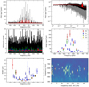 |
Fig. B.1 Summary of the peakbagging of the subgiant KIC 5723165. Top left: Original PSD as a function of frequency in a linear scale around vmax (grey), a smoothed PSD (black), and the resultant fit (red). Top right: Same three PSDs in a log-log scale. Central left: Residual of PSD (in S/N) after removing the fitted model. The coloured lines represent different levels of smoothing. Central right: Fitted mode heights as a function of frequency. Bottom left: Fitted mode widths as a function of frequency. Bottom right: Echelle diagram with a Δν of 34.3 µHz. Crosses indicate the fitted frequencies. This figure has been produced as one of apollinaire standard outputs. |
Table B.1 summarises the parameters obtained for the fitted modes.
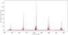 |
Fig. B.2 PSD of KIC 5723165 with the regions of the odd modes masked (grey line) and a smoothed version of this PSD in black. The red line corresponds to the result of fitting the Universal pattern. The structure between the modes ℓ=2 and ℓ=0 around 565 µHz is a mixed mode. |
Parameters fitted for KIC 5723165 modes.
Appendix C Detailed results from Kepler LEGACY targets
The detailed results of the p-mode individual parameters fitted for the benchmark on the six LEGACY targets performed in Sect. 4.3 are presented here. Table D.3 presents the comparison of H and Γ between apollinaire and L17. As L17 chose to fit amplitude rather than heights, the corresponding mode heights and uncertainties have been recomputed through the proxy of their Eq. 6. Table D.4 presents the comparison of mode frequencies ν and quality assurance factors ln K between apollinaire and L17.
Appendix D Input and output files
The apollinaire module is built around a certain number of input and output files which are described in the subsequent sections.
Appendix D.1 The a2z file and the a2z DataFrame
The syntax of the a2z files has been designed to specify some pieces of information the procedure has to be aware of when dealing with individual mode parameters extraction. A line corresponds to a parameter. The file contains nine columns: order n, degree ℓ, name of the parameter, extent, value, uncertainty σsym (see Sect. 3.1),fixed key, low bound and up bound of the parameter.
If a parameter has to apply to every order or degrees, the value to specify in the corresponding column is a. The possible parameters name are freq, height, width, asym, angle, split. Parameters with name freq, height or width cannot have n = a, parameters with name freq cannot have ℓ = a. The extent columns reminds the extent of application of a given parameter: mode, pair, order, or global. The pair keyword can only be used when fitting modes by pair. Only angle or split parameters can be set as global. For an input a2z file, the value column specify the value around where the sampler will initialise the walkers that will sample the MCMC. The uncertainty column is relevant only for output a2z files. It has to be read as the σy values given in Eq. 18. The fixed key column values must be set to 0 or 1 and are managed by the apollinaire function. Parameters with fixed key 0 at a given step will be fitted while parameters with 1-value will be read as frozen parameters. In input a2z files, the low bound and up bound columns specify the limit values inside which the posterior probability will be sampled. Obviously, the up bound must be greater than the low bound, and the value term must lay inside the defined interval.
An example of input for solar data is given in Table D.1. In apollinaire, a2z files are read as a2z DataFrame (pandas DataFrame with the structure specified in the previous paragraph) with the function read_a2z.
An example of helioseismic a2z input file corresponding to priors for the n = 20 GOLF order.
Appendix D.2 The pkb file and the pkb arrays
In pkb files, each line corresponds to a given mode of order n and degree ℓ. The file contains 14 columns: order n, degree ℓ, mode frequency ν, uncertainty over frequency σapprox,y mode height H, uncertainty over height σapprox,H,mode FWHM Γ, uncertainty over FWHM σapprox,Γ, stellar angle i, uncertainty over stellar angle σapprox,i, mode splitting s, uncertainty over mode splitting σapproxs, mode asymmetry α, uncertainty over mode asymmetry σapprox,α;. In Sect. 3.1, we describe the method used to compute σsym.
An example of helioseismic pkb file corresponding to fitted parameters for the n = 20 GOLF order.
An example of a pkb file is presented in Table D.2. In apollinaire procedures, pkb arrays (numpy arrays with the shape specified in the previous paragraph) are usually created by converting a2z DataFrame with the a2Z_to_pkb function. Those pkb arrays are used to build the models SSN(v) which are necessary to compute the likelihood and the posterior probability.
Appendix D.3 The extended pkb array
The structure of the extended pkb array is close to the classical pkb array structure, except that it contains 20 columns. Instead of σsym, two uncertainties values are provided for each parameters: σ− and σ+ (see Sect. 3.1).
Mode heights and widths obtained for modes fitted both in L17 and with apollinaire.
Mode frequencies and quality assurance factor ln K obtained for modes fitted both in L17 and with apollinaire.
References
- Ambikasaran, S., Foreman-Mackey, D., Greengard, L., Hogg, D. W., & O’Neil, M. 2015, IEEE Trans. Pattern Anal. Mach. Intell., 38, 252 [Google Scholar]
- Appourchaux, T. 2020, A&A, 642, A226 [NASA ADS] [CrossRef] [EDP Sciences] [Google Scholar]
- Appourchaux, T., Gizon, L., & Rabello-Soares, M. C. 1998, A&AS, 132, 107 [NASA ADS] [CrossRef] [EDP Sciences] [Google Scholar]
- Appourchaux, T., Samadi, R., & Dupret, M. A. 2009, A&A, 506, 1 [NASA ADS] [CrossRef] [EDP Sciences] [Google Scholar]
- Appourchaux, T., Chaplin, W. J., García, R. A., et al. 2012, A&A, 543, A54 [CrossRef] [EDP Sciences] [Google Scholar]
- Appourchaux, T., Antia, H. M., Benomar, O., et al. 2014, A&A, 566, A20 [NASA ADS] [CrossRef] [EDP Sciences] [Google Scholar]
- Astropy Collaboration (Robitaille, T. P., et al.) 2013, A&A, 558, A33 [NASA ADS] [CrossRef] [EDP Sciences] [Google Scholar]
- Astropy Collaboration (Price-Whelan, A. M., et al.) 2018, AJ, 156, 123 [Google Scholar]
- Auvergne, M., Bodin, P., Boisnard, L., et al. 2009, A&A, 506, 411 [NASA ADS] [CrossRef] [EDP Sciences] [Google Scholar]
- Ballot, J., García, R. A., & Lambert, P. 2006, MNRAS, 369, 1281 [Google Scholar]
- Ballot, J., Appourchaux, T., Toutain, T., & Guittet, M. 2008, A&A, 486, 867 [NASA ADS] [CrossRef] [EDP Sciences] [Google Scholar]
- Beck, P. G., Bedding, T. R., Mosser, B., et al. 2011, Science, 332, 205 [Google Scholar]
- Bedding, T. R., Mosser, B., Huber, D., et al. 2011, Nature, 471, 608 [Google Scholar]
- Benomar, O., Appourchaux, T., & Baudin, F. 2009, A&A, 506, 15 [NASA ADS] [CrossRef] [EDP Sciences] [Google Scholar]
- Benomar, O., Bedding, T. R., Stello, D., et al. 2012, ApJ, 745, L33 [NASA ADS] [CrossRef] [Google Scholar]
- Borucki, W. J., Koch, D. G., Basri, G., et al. 2011, ApJ, 736, 19 [Google Scholar]
- Breton, S. N., Santos, A. R. G., Bugnet, L., et al. 2021, A&A, 647, A125 [EDP Sciences] [Google Scholar]
- Breton, S. N., Pallé, P. L., García, R. A., et al. 2022, A&A, 658, A27 [NASA ADS] [CrossRef] [EDP Sciences] [Google Scholar]
- Broomhall, A. M., Chaplin, W. J., Elsworth, Y., Appourchaux, T., & New, R. 2010, MNRAS, 406, 767 [NASA ADS] [Google Scholar]
- Buzasi, D., Catanzarite, J., Laher, R., et al. 2000, ApJ, 532, L133 [Google Scholar]
- Chaplin, W. J., Elsworth, Y., Howe, R., et al. 1996, Sol. Phys., 168, 1 [NASA ADS] [CrossRef] [Google Scholar]
- Chaplin, W. J., Appourchaux, T., Arentoft, T., et al. 2008, Astron. Nachr., 329, 549 [NASA ADS] [CrossRef] [Google Scholar]
- Chaplin, W. J., Kjeldsen, H., Christensen-Dalsgaard, J., et al. 2011, Science, 332, 213 [Google Scholar]
- Christensen-Dalsgaard, J. 2008, Lecture Notes on Stellar Oscillations, 15th edn. https://phys.au.dk/~jcd/oscilnotes/ [Google Scholar]
- Collette, A. 2013, Python and HDF5 (O’Reilly) [Google Scholar]
- Conda-forge community 2015, https://10.5281/zenodo.4774217 [Google Scholar]
- Corsaro, E., & De Ridder, J. 2014, A&A, 571, A71 [NASA ADS] [CrossRef] [EDP Sciences] [Google Scholar]
- Corsaro, E., Grundahl, F., Leccia, S., et al. 2012, A&A, 537, A9 [NASA ADS] [CrossRef] [EDP Sciences] [Google Scholar]
- Corsaro, E., McKeever, J. M., & Kuszlewicz, J. S. 2020, A&A, 640, A130 [NASA ADS] [CrossRef] [EDP Sciences] [Google Scholar]
- Davies, G. R., Silva Aguirre, V., Bedding, T. R., et al. 2016, MNRAS, 456, 2183 [Google Scholar]
- Deheuvels, S., Ballot, J., Beck, P. G., et al. 2015, A&A, 580, A96 [NASA ADS] [CrossRef] [EDP Sciences] [Google Scholar]
- Duvall, T. L. J., Jefferies, S. M., Harvey, J. W., Osaki, Y., & Pomerantz, M. A. 1993, ApJ, 410, 829 [NASA ADS] [CrossRef] [Google Scholar]
- Dziembowski, W. 1977, Acta Astron., 27, 203 [NASA ADS] [Google Scholar]
- Fletcher, S. T., Chaplin, W. J., Elsworth, Y., Schou, J., & Buzasi, D. 2006, MNRAS, 371, 935 [NASA ADS] [CrossRef] [Google Scholar]
- Foreman-Mackey, D. 2016, J. Open Source Softw., 1, 24 [Google Scholar]
- Foreman-Mackey, D., Hogg, D. W., Lang, D., & Goodman, J. 2013, PASP, 125, 306 [Google Scholar]
- Fredslund Andersen, M., Pallé, P., Jessen-Hansen, J., et al. 2019, A&A, 623, L9 [NASA ADS] [CrossRef] [EDP Sciences] [Google Scholar]
- Fröhlich, C., Romero, J., Roth, H., et al. 1995, Sol. Phys., 162, 101 [Google Scholar]
- Gabriel, M. 1994, A&A, 287, 685 [NASA ADS] [Google Scholar]
- Gabriel, A. H., Grec, G., Charra, J., et al. 1995, Sol. Phys., 162, 61 [Google Scholar]
- García, R. A. 2015, in EAS Publications Series, 73-74, 193 [CrossRef] [EDP Sciences] [Google Scholar]
- García, R. A., & Ballot, J. 2019, Liv. Rev. Solar Phys., 16, 4 [CrossRef] [Google Scholar]
- García, R. A., Boumier, P., Charra, J., et al. 1999, A&A, 346, 626 [NASA ADS] [Google Scholar]
- García, R. A., Hekker, S., Stello, D., et al. 2011, MNRAS, 414, L6 [NASA ADS] [CrossRef] [Google Scholar]
- Gaulme, P., Appourchaux, T., & Boumier, P. 2009, A&A, 506, 7 [NASA ADS] [CrossRef] [EDP Sciences] [Google Scholar]
- Gizon, L., & Solanki, S. K. 2003, ApJ, 589, 1009 [Google Scholar]
- Goodman, J., & Weare, J. 2010, Commun. Appl. Math. Comput. Sci., 5, 65 [Google Scholar]
- Gruberbauer, M., & Guenther, D. B. 2013, MNRAS, 432, 417 [NASA ADS] [CrossRef] [Google Scholar]
- Gruberbauer, M., Kallinger, T., Weiss, W. W., & Guenther, D. B. 2009, A&A, 506, 1043 [NASA ADS] [CrossRef] [EDP Sciences] [Google Scholar]
- Gruberbauer, M., Guenther, D. B., MacLeod, K., & Kallinger, T. 2013, MNRAS, 435, 242 [CrossRef] [Google Scholar]
- Grundahl, F., Kjeldsen, H., Christensen-Dalsgaard, J., Arentoft, T., & Frandsen, S. 2007, Commun. Asteroseismol., 150, 300 [NASA ADS] [CrossRef] [Google Scholar]
- Grundahl, F., Fredslund Andersen, M., Christensen-Dalsgaard, J., et al. 2017, ApJ, 836, 142 [Google Scholar]
- Handberg, R., & Campante, T. L. 2011, A&A, 527, A56 [CrossRef] [EDP Sciences] [Google Scholar]
- Handberg, R., & Lund, M. N. 2014, MNRAS, 445, 2698 [Google Scholar]
- Harris, C. R., Millman, K. J., van der Walt, S. J., et al. 2020, Nature, 585, 357 [NASA ADS] [CrossRef] [Google Scholar]
- Harvey, J. 1985, in ESA Special Publication, Future Missions in Solar, Heliospheric & Space Plasma Physics, eds. E. Rolfe, & B. Battrick, 235, 199 [NASA ADS] [Google Scholar]
- Harvey, J. W., Hill, F., Hubbard, R. P., et al. 1996, Science, 272, 1284 [Google Scholar]
- Hastings, W. K. 1970, Biometrika, 57, 97 [Google Scholar]
- Hill, M. L., Kane, S. R., Campante, T. L., et al. 2021, AJ, 162, 211 [NASA ADS] [CrossRef] [Google Scholar]
- Houdayer, P. S., Reese, D. R., Goupil, M.-J., & Lebreton, Y. 2021, A&A, 655, A85 [NASA ADS] [CrossRef] [EDP Sciences] [Google Scholar]
- Howell, S. B., Sobeck, C., Haas, M., et al. 2014, PASP, 126, 398 [Google Scholar]
- Huber, D., White, T. R., Metcalfe, T. S., et al. 2022, AJ, 163, 79 [NASA ADS] [CrossRef] [Google Scholar]
- Hunter, J. D. 2007, Comput. Sci. Eng., 9, 90 [NASA ADS] [CrossRef] [Google Scholar]
- Jiménez-Reyes, S. J., Chaplin, W. J., García, R. A., et al. 2008, MNRAS, 389, 1780 [CrossRef] [Google Scholar]
- Kallinger, T., De Ridder, J., Hekker, S., et al. 2014, A&A, 570, A41 [NASA ADS] [CrossRef] [EDP Sciences] [Google Scholar]
- Kass, R. E., & Raftery, A. E. 1995, J. Am. Stat. Assoc., 90, 773 [Google Scholar]
- Kjeldsen, H., & Bedding, T. R. 1995, A&A, 293, 87 [NASA ADS] [Google Scholar]
- Kjeldsen, H., Bedding, T. R., Viskum, M., & Frandsen, S. 1995, AJ, 109, 1313 [NASA ADS] [CrossRef] [Google Scholar]
- Korzennik, S. G. 2005, ApJ, 626, 585 [NASA ADS] [CrossRef] [Google Scholar]
- Ledoux, P. 1951, ApJ, 114, 373 [Google Scholar]
- Liu, J. 2009, Monte Carlo Strategies in Scientific Computing (New York: Springer) [Google Scholar]
- Lund, M. N., Silva Aguirre, V., Davies, G. R., et al. 2017, ApJ, 835, 172 [Google Scholar]
- Mathur, S., García, R. A., Régulo, C., et al. 2010, A&A, 511, A46 [NASA ADS] [CrossRef] [EDP Sciences] [Google Scholar]
- Mathur, S., Huber, D., Batalha, N. M., et al. 2017, ApJS, 229, 30 [NASA ADS] [CrossRef] [Google Scholar]
- Mathur, S., García, R. A., Breton, S., et al. 2022, A&A, 657, A31 [NASA ADS] [CrossRef] [EDP Sciences] [Google Scholar]
- Matthews, J. M., Kuschnig, R., Walker, G. A. H., et al. 2000, in The Impact of Large-Scale Surveys on Pulsating Star Research, lAU Colloq. 176, eds. L. Szabados, & D. Kurtz, ASP Conf. Ser., 203, 74 [NASA ADS] [Google Scholar]
- Mazumdar, A., Monteiro, M. J. P. F. G., Ballot, J., et al. 2014, ApJ, 782, 18 [NASA ADS] [CrossRef] [Google Scholar]
- Metropolis, N., Rosenbluth, A. W., Rosenbluth, M. N., Teller, A. H., & Teller, E. 1953, J. Chem. Phys., 21, 1087 [Google Scholar]
- Mosser, B., Barban, C., Montalbán, J., et al. 2011, A&A, 532, A86 [NASA ADS] [CrossRef] [EDP Sciences] [Google Scholar]
- Mosser, B., Vrard, M., Belkacem, K., Deheuvels, S., & Goupil, M. J. 2015, A&A, 584, A50 [NASA ADS] [CrossRef] [EDP Sciences] [Google Scholar]
- Nielsen, M. B., Davies, G. R., Ball, W. H., et al. 2021, AJ, 161, 62 [NASA ADS] [CrossRef] [Google Scholar]
- Nigam, R., & Kosovichev, A. G. 1998, ApJ, 505, L51 [NASA ADS] [CrossRef] [Google Scholar]
- Oliphant, T. 2006, NumPy: A guide to NumPy (Trelgol Publishing) [Google Scholar]
- Pallé, P. L., Grundahl, F., Triviño Hage, A., et al. 2013, in Journal of Physics Conference Series, 440, 012051 [CrossRef] [Google Scholar]
- Pandas development team, T. 2020, https://10.5281/zenodo.3630805 [Google Scholar]
- Press, W. H., Teukolsky, S. A., Vetterling, W. T., & Flannery, B. P. 1992, Numerical recipes in FORTRAN. The art of scientific computing 2nd edn. (Cambridge University Press) [Google Scholar]
- Rauer, H., Catala, C., Aerts, C., et al. 2014, Exp. Astron., 38, 249 [Google Scholar]
- Ricker, G. R., Winn, J. N., Vanderspek, R., et al. 2015, J. Astron. Telescopes Instrum. Syst. 1, 014003 [Google Scholar]
- Salabert, D., Fossat, E., Gelly, B., et al. 2002, A&A, 390, 717 [NASA ADS] [CrossRef] [EDP Sciences] [Google Scholar]
- Salabert, D., Fossat, E., Gelly, B., et al. 2004, A&A, 413, 1135 [NASA ADS] [CrossRef] [EDP Sciences] [Google Scholar]
- Salabert, D., Chaplin, W. J., Elsworth, Y., New, R., & Verner, G. A. 2007, A&A, 463, 1181 [NASA ADS] [CrossRef] [EDP Sciences] [Google Scholar]
- Salabert, D., Ballot, J., & García, R. A. 2011a, in GONG-SoHO 24: A New Era of Seismology of the Sun and Solar-Like Stars, J. Phys. Conf. Ser., 271, 012053 [NASA ADS] [CrossRef] [Google Scholar]
- Salabert, D., Ballot, J., & García, R. A. 2011b, A&A, 528, A25 [NASA ADS] [CrossRef] [EDP Sciences] [Google Scholar]
- Salabert, D., García, R. A., & Turck-Chièze, S. 2015, A&A, 578, A137 [NASA ADS] [CrossRef] [EDP Sciences] [Google Scholar]
- Santos, A. R. G., García, R. A., Mathur, S., et al. 2019, ApJS, 244, 21 [Google Scholar]
- Santos, A. R. G., Breton, S. N., Mathur, S., & García, R. A. 2021, ApJS, 255, 17 [NASA ADS] [CrossRef] [Google Scholar]
- Scherrer, P. H., Bogart, R. S., Bush, R. I., et al. 1995, Sol. Phys., 162, 129 [Google Scholar]
- Scherrer, P. H., Schou, J., Bush, R. I., et al. 2012, Sol. Phys., 275, 207 [Google Scholar]
- Silva Aguirre, V., Lund, M. N., Antia, H. M., et al. 2017, ApJ, 835, 173 [Google Scholar]
- Smith, A. M. S., Breton, S. N., Csizmadia, S., et al. 2022, MNRAS, 510, 5035 [NASA ADS] [CrossRef] [Google Scholar]
- Sokal, A. 1997, Monte Carlo Methods in Statistical Mechanics: Foundations and New Algorithms, eds. C. DeWitt-Morette, P. Cartier, & A. Folacci (Boston, MA: Springer US), 131 [Google Scholar]
- Stahn, T., & Gizon, L. 2008, Sol. Phys., 251, 31 [NASA ADS] [CrossRef] [Google Scholar]
- Tassoul, M. 1980, ApJS, 43, 469 [Google Scholar]
- Tayar, J., Claytor, Z. R., Huber, D., & van Saders, J. 2022, ApJ, 927, 31 [NASA ADS] [CrossRef] [Google Scholar]
- Toutain, T., & Appourchaux, T. 1994, A&A, 289, 649 [NASA ADS] [Google Scholar]
- Toutain, T., & Gouttebroze, P. 1993, A&A, 268, 309 [NASA ADS] [Google Scholar]
- Toutain, T., Appourchaux, T., Fröhlich, C., et al. 1998, ApJ, 506, L147 [NASA ADS] [CrossRef] [Google Scholar]
- Unno, W., Osaki, Y., Ando, H., Saio, H., & Shibahashi, H. 1989, Nonradial oscillations of stars (Tokyo: University of Tokyo Press) [Google Scholar]
- Van Rossum, G., & Drake, F. L. 2009, Python 3 Reference Manual (Scotts Valley, CA: CreateSpace) [Google Scholar]
- Virtanen, P., Gommers, R., Oliphant, T. E., et al. 2020, Nature Methods, 17, 261 [CrossRef] [Google Scholar]
- Wes McKinney. 2010, in Proceedings of the 9th Python in Science Conference, eds. Stéfan van der Walt, & Jarrod Millman, 56 [CrossRef] [Google Scholar]
- White, T. R., Bedding, T. R., Stello, D., et al. 2011, ApJ, 742, L3 [Google Scholar]
- Woodard, M. F. 1984, PhD thesis, University of California, San Diego [Google Scholar]
For sake of completeness, the observation of α Ursae Majoris by the Wide-field InfraRed Explorer (WIRE, Buzasi et al. 2000) satellite must also be mentioned for its precursor role.
This paper describes the v1.1 of the module, for which additional documentation can be found at https://apollinaire.readthedocs.io/en/v1.1/
Originally developed inside the Kepler Asteroseismic Science Operations Center (KASOC) working package 6.
Full results, Kepler light curves, and data analysis tools used to perform the benchmark can be accessed through the following repository: https://gitlab.com/sybreton/benchmark_peakbagging_apollinaire
The GOLF time series used for this work can be downloaded at https://irfu.cea.fr/dap/LDEE/Phocea/Vie_des_labos/Ast/ast_visu.php?id_ast=3842
The mode frequency, amplitude and width tables are publicly available on VizieR at http://cdsarc.u-strasbg.fr/viz-bin/Cat?J/ApJ/835/172
KEPSEISMIC data are available at MAST via http://dx.doi.org/18.17909/t9-mrpw-gc07
This example is available on the same repository than the benchmark presented in Section 4: https://gitlab.com/sybreton/benchmark_peakbagging_apollinaire/-/tree/master/subgiant_recipe/5723165
All Tables
Percentage of values in the 68% and 99.7% credible intervals for the strong (ℓ = 0,1) mode in the Monte Carlo trial.
Percentage of values in the 68% and 99.7% credible intervals for the weak (ℓ = 2, 3) mode in the Monte Carlo trial.
KIC and fundamental stellar properties of selected targets from the LEGACY sample.
Comparison between vmax, Δν, and ϵ values yielded by apollinaire and reference values from L17.
An example of helioseismic a2z input file corresponding to priors for the n = 20 GOLF order.
An example of helioseismic pkb file corresponding to fitted parameters for the n = 20 GOLF order.
Mode heights and widths obtained for modes fitted both in L17 and with apollinaire.
Mode frequencies and quality assurance factor ln K obtained for modes fitted both in L17 and with apollinaire.
All Figures
|
Fig. 1 Top: Effects of the convolution by the Fourier transform of the observational window on an ideal Lorentzian mode profile (grey) in the case of continuous observations, with ΓTobs = 0.25 (red), 0.5 (dark blue), 0.75 (green), 1 (orange), 2 (light blue), and 5 (brown). Bottom: Same as top panel, but for the y-axis range [1, 2]. |
| In the text | |
|
Fig. 2 Model for a ℓ = 1, 3 pair with inclination angle i = 90° and splittings s = 0.4 µHz, without taking the observational window into account (grey) and the modified model with the observational window effect applied following Eq. (17) (orange). The actual convolution of the synthetic PSD by |ƒ|2 is represented in black for comparison. |
| In the text | |
|
Fig. 3 Simplified representation of the apollinaire flow chart. |
| In the text | |
|
Fig. 4 Summary of the available options for the p-mode individual parameter extraction step. |
| In the text | |
|
Fig. 5 Example of a synthetic spectrum generated with the pair 2 set of parameters and a frequency vector with 1460-day resolution (black). The ideal spectrum is overplotted in blue. |
| In the text | |
|
Fig. 6 Error νfitted – νtrue /σ on the ℓ = 1 mode from pair 2 and corresponding uncertainties for every Monte Carlo run with 365-day (grey) and 1460-day (blue) resolution. The zero vertical coordinate is highlighted by the red dashed line. |
| In the text | |
|
Fig. 7 Top: νfitted – νtrue distribution on the ℓ = 1 mode from pair 2 for every Monte Carlo run with 365-day (grey) and 1460-day (blue) resolution. Bottom: (νfitted – νtrue)/σ distribution on the ℓ = 1 mode from pair 2 for every Monte Carlo run with 365-day (grey) and 1460-day (blue) resolution. The mean value 〈(νfitted – νtrue)/σ〉 for both distributions is specified and the standard deviation of the 1460-day distribution is shown in red. |
| In the text | |
|
Fig. 8
|
| In the text | |
|
Fig. 9 L17 ϵ values (pentagons) compared to apollinaire ϵ values (stars) for the six considered targets. Corresponding KIC are specified next to each red dot. The epsilon values obtained by L17 for the other stars of the LEGACY sample are represented in grey. Some of the uncertainties are too small to be represented on the figure. |
| In the text | |
|
Fig. 10 Échelle diagram of the six selected targets apollinaire fitted p-mode frequencies (black diamonds) with corresponding error bars. The blue circles signal the frequency initial guesses inferred from Eq. (24). |
| In the text | |
|
Fig. 11 Comparison of p-mode frequencies yielded by apollinaire (dark blue) and reference values from L17 (light blue). The error bars overlapping intervals are represented in medium blue. The KEPSEISMIC PSD are represented in light grey while the apollinaire fitted model is shown in dark grey. |
| In the text | |
|
Fig. 12 Comparison of p-mode FWHMs and amplitudes yielded by apollinaire (dark blue and red, respectively) and reference values from L17 (light blue and salmon, respectively). The error bars overlapping intervals are represented in medium blue and dark salmon, respectively. |
| In the text | |
|
Fig. 13
|
| In the text | |
|
Fig. B.1 Summary of the peakbagging of the subgiant KIC 5723165. Top left: Original PSD as a function of frequency in a linear scale around vmax (grey), a smoothed PSD (black), and the resultant fit (red). Top right: Same three PSDs in a log-log scale. Central left: Residual of PSD (in S/N) after removing the fitted model. The coloured lines represent different levels of smoothing. Central right: Fitted mode heights as a function of frequency. Bottom left: Fitted mode widths as a function of frequency. Bottom right: Echelle diagram with a Δν of 34.3 µHz. Crosses indicate the fitted frequencies. This figure has been produced as one of apollinaire standard outputs. |
| In the text | |
|
Fig. B.2 PSD of KIC 5723165 with the regions of the odd modes masked (grey line) and a smoothed version of this PSD in black. The red line corresponds to the result of fitting the Universal pattern. The structure between the modes ℓ=2 and ℓ=0 around 565 µHz is a mixed mode. |
| In the text | |
Current usage metrics show cumulative count of Article Views (full-text article views including HTML views, PDF and ePub downloads, according to the available data) and Abstracts Views on Vision4Press platform.
Data correspond to usage on the plateform after 2015. The current usage metrics is available 48-96 hours after online publication and is updated daily on week days.
Initial download of the metrics may take a while.