© ESO 2022

1. Introduction

Massive stars have intense ultraviolet (UV) radiation fields that accelerate the surface material, launching powerful supersonic winds. These stellar winds interact with the interstellar medium (ISM), generating two shock fronts: a forward shock (FS) that propagates through the ISM and a reverse shock (RS) that propagates through the stellar wind (Weaver et al. 1977). These shocks are potential sites for non-thermal (NT) phenomena; they have been detected on a few occasions (Prajapati et al. 2019; Sánchez-Ayaso et al. 2018) and have been suggested to produce galactic cosmic rays up to PeV energies (e.g. Aharonian et al. 2019; Morlino et al. 2021).

Stars that have a supersonic velocity with respect to the local ISM are known as runaway stars. In this scenario, the interaction region becomes bow-shaped (van Buren & McCray 1988), and thus the whole interaction structure is usually called a bow shock (BS). The FS compresses and heats up dust and gas that emit mostly infrared (IR) and optical radiation (Peri et al. 2012; Kobulnicky et al. 2016), but BSs can also accelerate particles up to relativistic energies via diffusive shock acceleration (DSA). These particles, in turn, can interact with matter and electromagnetic fields, producing broadband NT radiation (as predicted by e.g. del Valle & Romero 2012; del Palacio et al. 2018; del Valle & Pohl 2018). Nonetheless, despite the fact that more than 700 BSs have been catalogued NT emission has been clearly detected only in one of them, BD+43°3654 (Benaglia et al. 2010, 2021). We note that radio emission has also been detected from the BS produced by the high-mass X-ray binary Vela X-1, but in this case the nature (thermal or NT) of the emission is still uncertain (van den Eijnden et al. 2022).

Hyper-velocity stars (HVSs) are the subclass of runaway stars with velocities of hundreds to a few thousands kms⁻¹ (Brown 2015). Recent observational campaigns have catalogued hundreds of HVSs with the data provided by Gaia, and models predict an ejection rate for HVSs of 10⁻⁴–10⁻⁵ yr⁻¹ (Zhang et al. 2013). Massive stars are promissory NT sources given that they are expected to develop strong BSs. The Hills mechanism (Hills 1988) explains the origin of HVSs via a three-body exchange between a stellar binary and a supermassive black hole. The black hole disrupts the binary, ejecting one of its components at great velocities. The velocity of ejection depends on the supermassive black hole mass and the total mass and semi-major axis of the binary. Recently this mechanism gained great support by the discovery of a ∼1700 km s⁻¹ A-type star ejected from Sgr A^* (Koposov et al. 2020).

Tutukov & Fedorova (2009) predicted a putative subclass of HVSs with semi-relativistic velocities, called semi-relativistic stars (SRSs). Numerical simulations support this prediction (Loeb & Guillochon 2016), and according to Dremova et al. (2017) a modified Hills mechanism can explain their origin. This mechanism consists of the gravitational interaction of two supermassive black holes that eject stars located in their central clusters. This mechanism predicts velocities of tens of thousands of km s⁻¹, with the maximum speed of ejection of the SRSs being determined by the mass of the secondary black hole and the mass of the ejected star (e.g. Guillochon & Loeb 2015).

In this work, we aim to characterise the NT particle production and associated emission spectra of BSs produced by massive stars that propagate with extreme velocities. In particular, we focus on massive HVSs and a putative SRS.

The paper is organised as follows. In Sect. 2, we present a multi-zone emission model that is suitable for extreme velocity stars for which the FS is also relevant. We present and discuss our results in Sect. 3, and finally, we conclude with a summary of the main findings of our work in Sect. 4.

2. Model

2.1. Scenarios studied

We define the fiducial cases to study keeping a compromise between the potential detectability of the sources and the feasibility of finding such objects. Regarding the luminosity of a BS produced by a massive star, the most important parameters are those associated with the properties of the stellar wind, and how they relate to the properties of the medium (del Palacio et al. 2018). We focus here particularly on massive stars in the main sequence, as this is the evolutionary stage in which they spend most of their life. These stars produce more powerful winds (and therefore more luminous BSs) for younger spectral types, although younger and more massive stars are less numerous (Salpeter 1955). In addition to stellar mass dependence, the energetics and radiation efficiency of the BS can also increase with the stellar spatial velocity (Martínez et al. 2021).

Observations with the Gaia satellite have detected several B-type stars with speeds over 100 km s⁻¹, but not a substantial quantity of O-type stars with those velocities (Kreuzer et al. 2020). According to Marchetti et al. (2019), the highest velocities found in HVSs are of the order of V_⋆ ∼ 10 000 km s⁻¹, although estimations above 1000 km s⁻¹ are unreliable. Putting everything together, we decided to study putative B0- and B1-type HVSs with velocities between 500 and 1000 km s⁻¹.

Within the scenarios of interest, we set the most promissory and less common stellar spectral type (B0) for the most conservative case, that is, a star with the lowest spatial velocity (500 km s⁻¹) propagating through the Galactic disk (d). For a B0 star, plausible wind parameters are Ṁ_w = 10⁻⁸ M_⊙ yr⁻¹ and v_w = 1500 km s⁻¹ (Krtička 2014; Kobulnicky et al. 2019). In addition, we consider HVSs with V_⋆ = 1000 km s⁻¹, Ṁ_w = 10⁻⁹ M_⊙ yr⁻¹, and v_w = 1200 km s⁻¹ propagating through three different media: the Galactic disk, the Galactic halo (h), and a molecular cloud (mc). This is motivated by the different densities in each of these media, easily reached by the HVSs, and the expectation that the FS is more luminous in a denser medium (Martínez et al. 2021). Lastly, we consider a B2 SRS with a spatial velocity of V_⋆ = 60 000 km s⁻¹, Ṁ_w = 10⁻¹⁰ M_⊙ yr⁻¹, and v_w = 1000 km s⁻¹, a viable scenario according to Dremova et al. (2017).

We summarise the characteristics of the selected scenarios in Table 1. Henceforth, we refer to the systems studied as <spectral type>  − <velocity of the star [in units of 10³ km s⁻¹]>  − <medium of propagation>. For instance, B1–1–d represents a B1 star propagating at 1000 km s⁻¹ through the Galactic disk.

2.2. Geometry

The BS forms as the result of the collision between the stellar wind and the ISM material. The former can be modelled as a spherical wind and the latter as a planar wind in the reference frame of the star. The FS propagates through the ISM and the RS propagates through the stellar wind, both separated by a contact discontinuity (CD). The shape of the CD is defined by the condition that the total momentum flows tangential to the shocked region, so that the flux of mass through the CD surface is null (Wilkin 1996; Christie et al. 2016). Each system is then divided into four regions: free-flowing stellar wind, unshocked ISM, shocked ISM, and shocked stellar wind, as represented in Fig. 1.

Fig. 1. Sketch of the model considered. The position of the CD is represented by a black solid line, while the orange and blue regions represent the FS and the RS, respectively. The solid lines with arrows represent different streamlines in each shock, injected in different positions separated by an angle Δθ. We also show the orientation of perpendicular and tangential vectors to the shocks in different positions, alongside vw and VISM = −V⋆, and the angle α between them. Adapted from del Palacio et al. (2018).

The DSA mechanism operates in strong and adiabatic shocks. For massive stars, the RS always fulfils these conditions given that radiative cooling is not efficient there (del Valle & Romero 2012). The FS, on the other hand, is radiative for typical runaway stars, but for the HVSs and SRSs considered in this work the FS is strong and adiabatic instead (see Sect. 2.3). Thus, both the RS and the FS are promissory accelerators of cosmic rays and are included in the model.

The closest position of the CD to the star, known as the stagnation point, is located along the axis of symmetry where the total pressures of the ISM and the stellar wind cancel each other out. The thermal pressure in both the ISM and the wind is negligible. Thus, the ISM total pressure (P_ISM) is

$$\begin{array}{c}\hfill P_{\mathrm{ISM}}={\rho }_{\mathrm{ISM}}{V}_{\star }^2,\end{array}$$(1)

where ρ_ISM is the density of the ISM. On the other hand, the total pressure of the stellar wind is given in terms of the mass-loss rate, the distance to the star, and the velocity of the wind:

$$\begin{array}{c}\hfill P_{\mathrm{w}}=\frac{{\dot{M}}_{\mathrm{w}}{v}_{\mathrm{w}}}{4\pi R{(\theta )}^2}.\end{array}$$(2)

Matching Eqs. (1) and (2), the stagnation point is located at

$$\begin{array}{c}\hfill R_0={\left[\frac{{\dot{M}}_{\mathrm{w}}{v}_{\mathrm{w}}}{4\pi {\rho }_{\mathrm{ISM}}{V}_{\star }^2}\right]}^{1/2}.\end{array}$$(3)

As it will be shown in the forthcoming Sect. 3, in the case of BSs from HVSs and SRSs, NT processes are relevant even at distant regions from the apex. Thus, a one-zone model approximation in which the emitter is considered homogeneous is not appropriate if one aims at more detailed quantitative predictions. Therefore, we adopt a multi-zone emission model based on the one developed by del Palacio et al. (2018), with the major difference being the incorporation of the FS in the model. For this, we follow an analogous approach as the one used for the RS in del Palacio et al. (2018) with some small modifications in the hydrodynamics.

Each shock in the BS is treated as a 2D structure. Neglecting the width of the shocked gas layers, these are co-spatial with the CD¹. The shape of the CD is calculated using the formulae given by Wilkin (1996). We assume that the shocked gas flows downstream at a fixed angle ϕ around the symmetry axis, dragging away NT particles. We model the 2D structure as a sum of 1D linear emitters embedded in the 3D physical space. For a given angle ϕ there are several 1D emitters, each starting at a different angle θ with respect to the symmetry axis where relativistic particles are injected, and consisting of multiple cells located along the path of the 1D emitter on the CD. Particles enter in the BS and are accelerated in the first cell of each 1D emitter, and then they move to the following cells up to an angle θ_max (Fig. 1). All the 1D emitters at a certain angle ϕ are summed up, thereby obtaining a 1D structure that contains all the relativistic particles along a shock at that particular angle. Finally, we rotate this 1D structure made of all the 1D emitters with the same ϕ value around the symmetry axis to get the full 2D structure of the BS. At last, we note that in all the scenarios we study, the stellar velocity is significantly below the speed of light. Therefore, relativistic effects in the hydrodynamics, as well as in the calculation of the NT particle distribution at each cell and the radiation they produce (e.g. Doppler boosting), can be neglected.

2.3. Hydrodynamics

We introduce here the semi-analytical hydrodynamical model used to characterise the properties of the shocked gas in the BS. In del Palacio et al. (2018), Rankine-Hugoniot jump conditions were assumed, which near the apex yields correct values up to first order. Here, we adopt a more consistent approach that is suitable to model both the RS and the FS up to distant regions from the BS apex. Firstly, we assume that the total pressure at R₀ is the ambient total pressure. Secondly, we consider Bernoulli’s equation across the shock:

$$\begin{array}{c}\hfill \frac{1}{2}{v}_{\mathrm{u}}^2+\left(\frac{{\gamma }_{\mathrm{ad}}}{{\gamma }_{\mathrm{ad}}-1}\right)\frac{P_{\mathrm{th},\mathrm{u}}(\theta )}{{\rho }_{\mathrm{u}}(\theta )}=\frac{1}{2}v{(\theta )}^2+\left(\frac{{\gamma }_{\mathrm{ad}}}{{\gamma }_{\mathrm{ad}}-1}\right)\frac{P_{\mathrm{th}}(\theta )}{\rho (\theta )},\end{array}$$(4)

where we labelled the upstream region with the subscript u. Given that R₀ ≫ R_⋆ for the scenarios considered here (Table 1), we adopt v_w = v_∞. Then, v_u is equal to v_∞ in the RS, and equal to V_⋆ in the FS. Moreover, we neglect the thermal pressure in the upstream region when compared to the ram (kinetic) pressure, since $P_{\text{th},\text{u}}\ll P_{\text{ram},\text{u}}\propto v_{\text{u}}^2$. The incoming stellar wind and ISM impact perpendicularly to the BS apex, where the fluid halts. Hereafter, we represent quantities at the stagnation point (θ = 0) with a subscript 0. Using Eq. (4), we determine the density at the stagnation point as

$$\begin{array}{c}\hfill {\rho }_0=\left(\frac{{\gamma }_{\mathrm{ad}}}{{\gamma }_{\mathrm{ad}}-1}\right)\frac{2P_{\mathrm{th}0}}{v_{\mathrm{u}}^2}=5\frac{P_{\mathrm{th}0}}{v_{\mathrm{u}}^2}=5{\rho }_{\mathrm{u}},\end{array}$$(5)

assuming that the fluid behaves like an ideal gas with adiabatic coefficient γ_ad = 5/3.

We assume that the shocked gas moves parallel to the CD. In the regions where the shocked fluid is subsonic, the flux of momentum that crosses the shock perpendicularly heats the downstream material, converting the total pressure in the upstream into thermal pressure in the downstream. We can thus calculate the total pressure at each point as

$$\begin{array}{c}\hfill P(\theta )=P_{\mathrm{th}}(\theta )={\rho }_{\mathrm{u}}(\theta )v_{\mathrm{u}}{v}_{\mathrm{u}\perp }(\theta ).\end{array}$$(6)

On the other hand, if the fluid becomes supersonic at an angle θ_c, we consider that only the momentum density component perpendicular to the BS that crosses the BS also perpendicularly is converted to thermal energy. This two-region approach requires adopting a soft transition of the thermodynamic quantities between both regimes. We thus adopt a prescription for the total pressure for θ > θ_c of the form

$$\begin{array}{c}\hfill P(\theta )=P_{\mathrm{th}}(\theta )={\rho }_{\mathrm{u}}(\theta )\left(\frac{v_{\mathrm{u}}}{v_{\mathrm{u}\perp }({\theta }_{\mathrm{c}})}\right)v_{\mathrm{u}\perp }{(\theta )}^2.\end{array}$$(7)

We can then calculate the density using the politropic relation:

$$\begin{array}{c}\hfill \rho (\theta )={\rho }_0{\left(\frac{P(\theta )}{P_0}\right)}^{1/{\gamma }_{\mathrm{ad}}}.\end{array}$$(8)

However, at large values of θ this underestimates the fluid density, so we impose the condition ρ(θ)≥ρ_min(θ), where ρ_min is defined as

$$\begin{array}{c}\hfill {\rho }_{\min }(\theta )=\{\begin{array}{c}{\rho }_{\mathrm{u}}\mathrm{FS}\hfill \\ (\frac{4\pi }{\mathrm{\Omega }(\pi -\theta )}-1){\rho }_{\mathrm{u}}\mathrm{RS},\hfill \end{array}\end{array}$$(9)

with Ω(x) = 2π(1−cos(x)), which takes into account the fraction of stellar wind accumulated in the RS up to an angle θ. To derive these expressions we have assumed that the shocked flow behaves as only one stream line that at each location adapts to the impact of the incoming upstream material, having homogeneous conditions in the direction perpendicular to the CD. This approximation is valid in the subsonic region, although it weakens in the supersonic region as the shocked flow is not causally connected along the CD.

The assumption of a laminar flow requires the suppression of dynamical instabilities, such as Rayleigh-Taylor (triggered by density differences across the CD) and Kelvin-Helmholtz instabilities (triggered by tangential velocity differences across the CD). Such instabilities can arise in stellar BSs, especially when the ambient medium is dense (e.g. Comeron & Kaper 1998; Meyer et al. 2016), although a high stellar velocity inhibits their appearance up to θ ≳ 135° (Comeron & Kaper 1998; Christie et al. 2016). Neglecting instabilities is further justified in the presence of adiabatic shocks (e.g. Falceta-Gonçalves & Abraham 2012), as it is the case in the context of HVSs and SRSs.

A shock is considered adiabatic when the gas escapes from the shock region before it cools significantly. This condition can be expressed as t_th/t_conv ≳ 1, with

$$\begin{array}{c}\hfill t_{\mathrm{th}}(\theta )=\frac{k_{\mathrm{B}}{\mathrm{\mu }}_{\mathrm{u}}{m}_{\mathrm{p}}T}{\zeta (\theta ){\rho }_{\mathrm{u}}\lambda (T)},\end{array}$$(10)

where the function λ(T) depends on the temperature of the shock (Myasnikov et al. 1998), and m_p is the proton mass. For the convection timescale we use the expression given in del Palacio et al. (2018), t_conv = R(θ)/v_∥(θ). In Fig. 2 we show the logarithm of the ratio t_th/t_conv as a function of the angle θ for the FSs. This ratio increases with θ up to θ ∼ 45° in the HVSs and up to θ ∼ 70° in the SRS as the fluid accelerates. After this, the ratio slowly decreases as t_conv ∝ R(θ) increases. As a result, the FS is adiabatic up to θ ∼ 160° in the systems B1–1–d and B1–1–mc, and up to θ ∼ 135° in the system B0–05–d (see Fig. 2). Moreover, the FS of the systems B1–1–h and B2–60–d, as well as the RSs in all cases studied, always fulfil the adiabaticity condition.

Fig. 2. Logarithm of the ratio tth/tconv for the different FSs studied in this work. For reference, we plot a black dotted horizontal line at zero (where tth = tconv); curves above this line corresponds to adiabatic shocks.

Lastly, the magnetic field in the subsonic regime (θ < θ_c) is obtained imposing that, at each position, its pressure is a fraction, η_B, of the thermal pressure of the shocked region:

$$\begin{array}{c}\hfill B(\theta )={\left({\eta }_{\mathrm{B}}8\pi P_{\mathrm{th}}(\theta )\right)}^{1/2}.\end{array}$$(11)

In the supersonic regime (θ > θ_c), we assume that the magnetic field remains frozen to the plasma, and that it is tangent to the shock surface. The later assumption is motivated by the fact that the magnetic field component perpendicular to the shock normal is amplified by adiabatic compression, and thus in general it should be the dominant component in both shocks (RS and FS).

We can then obtain the magnetic field as

$$\begin{array}{c}\hfill B(\theta )=B({\theta }_{\mathrm{c}}){\left(\frac{\rho (\theta )}{\rho ({\theta }_{\mathrm{c}})}\frac{v({\theta }_{\mathrm{c}})}{v(\theta )}\right)}^{1/2}.\end{array}$$(12)

In Fig. 3 we show the dependence of the thermodynamic quantities with θ for both shocks. In the apex the conversion of kinetic energy to internal energy is maximised as the shock is perpendicular. The tangential velocity increases monotonically with θ, going from zero in the stagnation point to v_t ∼ v_∞ in the RS and v_t ∼ V_⋆ in the FS. The pressure slowly decays with θ in the FS, while it drops more abruptly in the RS because P_RS ∝ ρ_w ∝ R⁻²; as a consequence, the other quantities that depend on P also decay gradually. We highlight that the magnetic field decreases slowly in the FS, which favours synchrotron emission up to large values of θ. Lastly, we note that this hydrodynamic model yields densities along the shocks that are slightly higher than the ones obtained assuming Rankine-Hugoniot jump conditions. The discrepancy is a factor of ∼1.5 for angles θ ≲ 60°, and a factor of ∼2 in the distant regions with θ > 60° (see Fig. A.1). The reason for this is that, as explained above, different regions of the shocked layer affect each other making the local hydrodynamical conditions depart from the Rankine-Hugoniot ones.

Fig. 3. Left panel: thermodynamic variables in the RS as a function of the position angle along the shock. We also give as a reference the linear distance along the shock, $\mathrm{\Delta }s={\int }_0^{\theta }\text{d}l$. The sub-index 0 refers to values in the apex. Right panel: same but for the FS.

2.4. Non-thermal particles

Relativistic particles can be accelerated via DSA in hypersonic and adiabatic shocks, such as the ones present in the BS (Sect. 2.3). Additionally, both electrons and protons could be accelerated via shock drift acceleration (SDA) in the RS, as the stellar magnetic field lines are expected to be parallel to the shock surface (Marcowith et al. 2016). Nevertheless, acquiring relativistic energies through SDA requires multiple interactions with the shock front, similarly to DSA (Matthews et al. 2020). Given that both mechanisms lead to the injection of a power-law distribution of particles and we treat the acceleration details phenomenologically, we refer in what follows only to acceleration via DSA although SDA might be also involved.

The energy distribution of the injected particles at the ith cell is assumed to be

$$\begin{array}{c}\hfill Q(E,{\theta }_i)=Q_0{E}^{-p}exp(-E/E_{\max }),\end{array}$$(13)

where Q₀ is a normalisation factor, p is the spectral index, and E_max is the cut-off energy, all dependent on θ_i.

The normalisation constant Q₀ is set by the condition ∫EQ(E, θ_i) dE = ΔL_NT(θ_i), being ΔL_NT(θ_i) the power available to accelerate NT particles at each position. That is,

$$\begin{array}{c}\hfill \mathrm{\Delta }{L}_{\mathrm{NT}}({\theta }_i)=f_{\mathrm{NT}}\mathrm{\Delta }{L}_{\perp }({\theta }_i)=f_{\mathrm{NT}}{S}_{\mathrm{E}}({\theta }_i)A_{\perp }({\theta }_i),\end{array}$$(14)

where S_E(θ_i) is the energy flux per unit volume of the corresponding fluid, and A_⊥(θ_i) is the area of the cell surface projected perpendicular to v_u. This area is calculated as A_⊥(θ_i) = R(θ_i) sin(θ_i) Δl(θ_i) sin(α_i) Δϕ, with Δl(θ_i) being the length of the cell and α_i the angle between v_u and the tangent to the shock, T (Fig. 1). The parameter f_NT is defined as the fraction of the power injected to the BS that goes to NT particles. We adopt f_NT = 0.1 and assume that 95% of this power goes to protons, while the remaining 5% goes to electrons. Finally, the energy flux per unit volume in the subsonic regime is $S_{\text{E}}=0.5{\rho }_{\text{u}}{v}_{\text{u}}^3$, whereas in the supersonic regime only the perpendicular velocity component is converted into thermal energy and therefore $S_{\text{E}}=0.5{\rho }_{\text{u}}{v}_{\text{u}}^2{v}_{\text{u}\perp }$. Contrary to what happens in the RS, the injection of energy in the FS is relevant even at large values of θ, where the flow is more susceptible to developing instabilities. That could potentially increase the area of the shock, thus enhancing the injected power and, consequently, the emitted luminosity (e.g. de la Cita et al. 2017). Nevertheless, the variability induced by this effect is not expected to dominate the average luminosities predicted in our model.

We can determine p in terms of the compression factor ζ as (e.g. Caprioli & Spitkovsky 2014)

$$\begin{array}{c}\hfill p({\theta }_i)=\frac{\zeta ({\theta }_i)+2}{\zeta ({\theta }_i)-1},\zeta ({\theta }_i)=\left(\frac{{\gamma }_{\mathrm{ad}}+1}{{\gamma }_{\mathrm{ad}}}\right)\frac{M{({\theta }_i)}^2}{M{({\theta }_i)}^2+2},\end{array}$$(15)

where M is the Mach number. Finally, E_max is obtained by equating the acceleration and energy loss timescales.

The steady-state particle distribution at the injection cell is

$$\begin{array}{c}\hfill N_0(E,{\theta }_i)\approx Q(E,{\theta }_i)\times \min (t_{\mathrm{cell}},t_{\mathrm{cool}}),\end{array}$$(16)

where t_cell the cell convection time and t_cool the cooling timescale. In the BS, electrons cool mainly by synchrotron and inverse Compton (IC) interactions, the latter with both the stellar UV (IC_⋆) and dust IR (IC_IR) radiation fields (Martínez et al. 2021). Adiabatic losses can also be relevant, whereas relativistic Bremsstrahlung losses are negligible. Protons cool by proton-proton inelastic collisions, a rather minor effect, and adiabatic losses.

The NT particles are confined within the shock and so they are dragged by the fluid. This occurs because the particles gyro-radii, r_g(E, θ)∝E/B(θ), even for E ∼ E_max are much smaller than the shocked layer width (the shock typical scale) H(θ). The latter is calculated considering mass conservation across the shock,

$$\begin{array}{c}\hfill H(\theta )=\frac{{\int }_0^{\theta }{\rho }_{\mathrm{u}}({\theta }^{\prime })v_{\mathrm{u}}{A}_{\perp }({\theta }^{\prime })\mathrm{d}{\theta }^{\prime }}{2\pi R(\theta )sin(\theta )\rho (\theta )v_{\Vert }(\theta )},\end{array}$$(17)

yielding a typical value of H(θ)∼0.3R(θ) for θ < π/2 (Christie et al. 2016). If we consider that there is a certain number of NT particles with energy E in the ith cell, by the time they reach the (i+1)th cell their energy will be E′≤E, and the size and convection velocity of the cell will also be different. Nonetheless, in the steady-state, the flux of particles in the position and energy space must be conserved. Considering this, we obtain the evolution of the particle energy distribution along a linear emitter²:

$$\begin{array}{c}\hfill N(E^{\prime },i+1)=N(E,i)\frac{|\dot{E}(E,i+1)|}{|\dot{E}(E^{\prime },i+1)|}\frac{t_{\mathrm{cell}}(i+1)}{t_{\mathrm{cell}}(i)},\end{array}$$(18)

with |Ė(E,i)| = E/t_cool(E,i) the cooling rate for particles of energy E at the position θ_i and t_cell(i) the convection time of the ith cell. Finally, the energy E′ is given by the condition $t_{\mathrm{cell}}={\int }_E^{E^{\prime }}\dot{E}(\stackrel{\sim }{E},i)\mathrm{d}\stackrel{\sim }{E}$.

We use the formulae given by Khangulyan et al. (2014) to calculate the isotropic IC cooling timescales, given that the electron distribution is isotropic at each position and the fluid is non-relativistic. These expressions take into account the Klein-Nishina (K-N) cross section for the interaction at high energies. For the case of the stellar radiation field, we consider the star as a black body emitter with temperature T_⋆ and a dilution factor of the photon field κ_⋆ = [R_⋆/(2R(θ))]². For the case of the IR photon field produced by the dust, we assume isotropy within the NT emitter, and we approximate its spectrum with a Planck law of temperature T_IR = 100 K. The corresponding dilution factor is κ_IR(θ) = U_IR(θ)/U_BB, where U_BB is the energy density of the radiation of a black body with temperature T_IR. Since U_IR ≈ L_IR/(4πR(θ)²c) (considering that the dust is concentrated in a thin shell surrounding the BS) and $U_{\text{BB}}=4\sigma T_{\text{IR}}^4/c$, we obtain

$$\begin{array}{c}\hfill {\kappa }_{\mathrm{IR}}=\frac{L_{\mathrm{IR}}}{16\pi \sigma T_{\mathrm{IR}}^{4}R{(\theta )}^2}.\end{array}$$(19)

3. Results

First, we compute the timescales and particle energy distributions for the scenarios studied. Then, we use a one-zone model to estimate the luminosity scaling with the relevant parameters of the systems. Finally, we present the spectral energy distributions (SEDs), and discuss the detectability of each system.

The magnetic field in the shocked region can be generated by adiabatic compression of the ISM (star) magnetic field in the FS (RS) and/or be amplified by the action of cosmic rays. Adopting η_B = 0.1 in Eq. (11) yields values of B consistent with a ratio between NT energy density and magnetic energy density of U_NT/U_B ≳ 1. Thus, in both shocks the magnetic field could be the result of amplification by cosmic rays (Bell 2004). Alternatively, in the RS the magnetic field could come from adiabatic compression of the stellar magnetic field. Under these conditions, and adopting an Alfvén radius r_A ∼ R_⋆, the stellar magnetic field in the stellar surface is B_⋆ ∼ 0.25 B(θ) (R(θ)/R_⋆) (v_∞/v_rot), with the star rotation speed being v_rot ∼ 0.1 v_∞ (del Palacio et al. 2018). We obtain B_⋆ ∼ 25 G for the B0 star, B_⋆ ∼ 10 G for the B1 stars, and B_⋆ ∼ 3 G for the B2 star. Given that these are plausible values (Parkin et al. 2014), adopting η_B = 0.1 is a reasonable assumption. Additionally, we consider an equipartition scenario (η_B = 1) to set an upper limit to the predicted radio fluxes. At last, given that the majority of power is injected within θ < 170°, and that instabilities can be significant for large values of θ, we fix θ_max = 170°.

3.1. Relativistic particle population

In Table 2 we show the power injected in NT particles (both electrons and protons) for each scenario. This quantity increases with younger spectral types and the velocity of the star, as expected from Eq. (14). Considering that there are at most tens of thousands of HVSs in the Milky Way (Marchetti et al. 2019), the total luminosity injected in NT particles by these sources in the Galaxy is likely below 10³⁸ erg s⁻¹. Then, HVSs do not significantly contribute to the Galactic cosmic ray population, which has a much larger (by a factor of ∼10³) contribution from supernova remnants.

3.1.1. Forward shock

An example of the timescales considered is shown in Figs. 4 and 5 for the FS of the system B1–1–d. For electrons near the apex, convection (escape) dominates up to E_e ≤ 4 GeV. In the range 4 GeV ≤ E_e ≲ 160 GeV, IC losses with the stellar photon field are dominant, also versus IR IC losses; these interactions occur in the Thomson regime for E_e ≲ 30 GeV, and in the K-N regime for E_e ≳ 30 GeV. At last, diffusion (escape) losses dominate above 160 GeV, and electrons reach energies of E_e, max ∼ 500 GeV. In a scenario with a lower ISM density (system B1–1–h), the stagnation point is further from the star, and so the density of stellar photons in the BS is smaller. As a consequence, IC timescales are larger, and convection losses are dominant up to E_e ≲ 100 GeV, and diffusion losses are dominant in the range 100 GeV ≲ E_e ≲ 300 GeV ∼ E_e, max. Similarly, R₀ also increases for main-sequence stars with younger spectral types, as Ṁ_w and v_w increase. Finally, for a SRS (B2–60–d), R₀ is significantly closer to the star (R₀ ≈ 30 R_⋆). Then, IC_⋆ interactions are dominant for 3 GeV ≤ E_e ≲ 600 GeV, and IC_IR interactions are dominant in the range 600 GeV ≲ E_e ≲ 2 TeV. Above E_e ≥ 2 TeV and up to E_max diffusion dominates. Since $B(\theta )\propto P(\theta )\propto V_{\star }^2\gg 1000$ km s⁻¹, the acceleration of NT particles is very efficient, yielding maximum energies of E_e, max ∼ 5 TeV for electrons and E_p, max ∼ 10 TeV for protons.

Fig. 4. Cooling times for three different positions of electrons for the FS of the system B1–1–d. The IC cooling timescale of electrons takes into account both the stellar and dust photon fields.

Fig. 5. Cooling times for protons of the system B1–1–d near the apex.

In distant regions from the apex, the stellar photon field is more diluted and therefore IC losses are less important. Additionally, the convection timescale shortens as v_∥ increases. As a consequence, convection losses are completely dominant in the FS of all systems for angles θ ≳ 100°. Moreover, particle acceleration is less efficient in distant regions since both v_⊥ and B decrease with θ (Fig. 3). Then, E_max diminishes with θ for both electrons and protons.

In contrast, protons are convected away from the FS without radiating a significant fraction of their energy. For the HVSs, close to the apex convection losses are the dominant process for protons with E_p < 160 GeV. In the case of the SRS (scenario B2–60–d), convection dominates up to E_p ≳ 1 TeV³. Above the energies mentioned, and up to E_p, max, diffusion losses are dominant.

Protons reach their maximum energy at the apex (θ = 0). We estimate the scaling of E_{p, max, 0} with the system parameters by matching t_ac, 0(E_p) = t_diff, 0(E_p). Considering diffusion in the Bohm regime, these timescales are

$$\begin{array}{cc}& t_{\mathrm{ac},0}(E_{\mathrm{p}})=\frac{2\pi c}{q}\frac{E_{\mathrm{p}}}{B_0{v}_{\perp 0}}=\frac{2\pi c}{q}\frac{E_{\mathrm{p}}}{B_0{v}_{\mathrm{u}}},\hfill \end{array}$$(20)

$$\begin{array}{cc}\hfill & t_{\mathrm{diff},0}(E_{\mathrm{p}})=\frac{R_0^2}{2D_{\mathrm{B},0}}=\frac{3q}{2c}\frac{R_0^2{B}_0}{E_{\mathrm{p}}},\hfill \end{array}$$(21)

where c, q, and D_B are the speed of light, proton charge, and diffusion coefficient, respectively. Finally, using Eqs. (6) and (11), we get $E_{\max ,\mathrm{p},0}\propto R_0{B}_0{V}_{\star }^{0.5}\propto {\dot{M}}_{\mathrm{w}}^{0.5}{v}_{\mathrm{w}}^{0.5}{V}_{\star }^{0.5}$. This maximum energy is E_max, p ∼ 1 TeV for the HVSs and E_max, p ∼ 10 TeV for the SRS.

When convection dominates, particles move along the BS with an energy distribution that keeps the same spectral index as the injected distribution. On the other hand, when IC in the Thomson regime or diffusion dominates, the particle energy distribution is softened. In Fig. 6 we show the particle energy distribution of electrons and protons in different regions of the RS and the FS for the system B1–1–d.

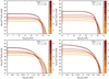Fig. 6. Particle energy distribution for electrons (top panels) and protons (bottom panels). The left panels are for the RS and the right panels are for the FS. The colour scale represents five different regions of the emitter that correspond to intervals of length Δθ = θmax/5 = 34°. The black dashed line corresponds to the total particle energy distribution.

3.1.2. Reverse shock

Characteristic timescales near the apex for the RS are similar to the ones of the FS of the HVSs. Nonetheless, the behaviour is different for the SRS. Despite the acceleration timescale decreases as the magnetic field is strengthens, the IC cooling timescale decreases more drastically, yielding maximum electron energies of E_e, max ∼ 10 GeV in the RS (the RS shock velocity is much lower than in the FS). Moreover, we highlight that IC cooling is still relevant up to θ ∼ 160° for the RS of this system.

Finally, matching Eqs. (20) and (21) for the RS we find for protons that $E_{\max ,\mathrm{p}}(0)\propto R_0{B}_0{V}_{\mathrm{w}}^{0.5}\propto {\dot{M}}_{\mathrm{w}}^{0.5}{v}_{\mathrm{w}}$. In this case, the maximum energy is E_{max, p, 0} ≳ 1 TeV for the HVSs and E_{max, p, 0} ∼ 200 GeV for the SRS.

3.2. Analytical estimates on emissivity scaling

A one-zone approximation is suitable to obtain order-of-magnitude estimates of the radiative outputs, with the advantage that the dependences of the emission with respect to different system parameters become explicit (e.g. del Palacio et al. 2018). We therefore apply this formalism to derive the scaling of the BS luminosity with the relevant system parameters.

We consider that the BS has an effective surface of size R_eff = a R₀. This is mostly relevant for the FS, for which a ∼ 5 (as explained below), whereas for the RS it is a ∼ 1. If t_rad is the cooling timescale of the dominant NT mechanism in a certain energy range, we estimate the NT power emitted in that range by each shock as

$$\begin{array}{c}\hfill L_{\mathrm{rad}}\sim L_{\mathrm{NT}}\left(\frac{t_{\mathrm{conv}}}{t_{\mathrm{rad}}}\right)\propto \{\begin{array}{cc}f(a){\dot{M}}_{\mathrm{w}}{v}_{\mathrm{w}}^2\left(\frac{t_{\mathrm{conv}}}{t_{\mathrm{rad}}}\right)\hfill & \mathrm{RS}\hfill \\ {\rho }_{\mathrm{ISM}}{R}_{\mathrm{eff}}^2{V}_{\star }^3\left(\frac{t_{\mathrm{conv}}}{t_{\mathrm{rad}}}\right)\hfill & \mathrm{FS},\hfill \end{array}\end{array}$$(22)

where f(a) is an order unity function that tends to f(a)≈0.6 as a increases. Qualitatively, the ratio t_conv/t_syn determines the NT luminosity emitted in the radio band. On the other hand, γ-ray emission depends on the ratio t_conv/t_IC⋆, as IC process with the stellar radiation field is the dominant NT process for those energies. We mote that these timescale-ratio dependences of the radiation luminosity are strictly valid for a dominant t_conv.

The convection (escape) timescale is roughly determined by the effective radius and the sound speed in the shocked gas:

$$\begin{array}{c}\hfill t_{\mathrm{conv}}\sim \frac{R_{\mathrm{eff}}}{c_{\mathrm{s}}}\propto \{\begin{array}{cc}a{\dot{M}}_{\mathrm{w}}^{0.5}{v}_{\mathrm{w}}^{-0.5}{n}_{\mathrm{ISM}}^{-0.5}{\mathrm{\mu }}_{\mathrm{ISM}}^{-0.5}{V}_{\star }^{-1}\hfill & \mathrm{RS}\hfill \\ \hfill \\ a{\dot{M}}_{\mathrm{w}}^{0.5}{v}_{\mathrm{w}}^{0.5}{n}_{\mathrm{ISM}}^{-0.5}{\mathrm{\mu }}_{\mathrm{ISM}}^{-0.5}{V}_{\star }^{-2}\hfill & \mathrm{FS}.\hfill \end{array}\end{array}$$(23)

On the other hand, the synchrotron cooling timescale is (e.g. Blumenthal & Gould 1970)

$$\begin{array}{c}\hfill t_{\mathrm{syn}}\propto B^{-2}\propto \{\begin{array}{cc}{\left({\dot{M}}_{\mathrm{w}}{v}_{\mathrm{w}}{R}_{\mathrm{eff}}^{-2}\right)}^{-1}\propto a^2{n}_{\mathrm{ISM}}^{-1}{\mathrm{\mu }}_{\mathrm{ISM}}^{-1}{V}_{\star }^{-2}\hfill & \mathrm{RS}\hfill \\ {\left({\rho }_{\mathrm{ISM}}{V}_{\star }^2\right)}^{-1}\propto n_{\mathrm{ISM}}^{-1}{\mathrm{\mu }}_{\mathrm{ISM}}^{-1}{V}_{\star }^{-2}\hfill & \mathrm{FS}.\hfill \end{array}\end{array}$$(24)

Thus, from Eqs. (22)–(24) we obtain

$$\begin{array}{c}\hfill L_{\mathrm{syn}}\sim L_{\mathrm{NT}}\left(\frac{t_{\mathrm{conv}}}{t_{\mathrm{syn}}}\right)\propto \{\begin{array}{cc}f(a)a^{-1}{\dot{M}}_{\mathrm{w}}^{1.5}{v}_{\mathrm{w}}^{1.5}{n}_{\mathrm{ISM}}^{0.5}{\mathrm{\mu }}_{\mathrm{ISM}}^{0.5}{V}_{\star }\hfill & \mathrm{RS}\hfill \\ \hfill \\ a^3{\dot{M}}_{\mathrm{w}}^{1.5}{v}_{\mathrm{w}}^{1.5}{n}_{\mathrm{ISM}}^{0.5}{\mathrm{\mu }}_{\mathrm{ISM}}^{0.5}{V}_{\star }\hfill & \mathrm{FS}.\hfill \end{array}\end{array}$$(25)

Therefore, synchrotron emission depends mostly on the stellar parameters: massive stars are promissory radio emitters, as they have fast, powerful winds. To a lesser extent, synchrotron luminosity increases with the speed of the star and the medium density. Finally, we note that the FS luminosity has a stronger dependence on the effective radius of the BS than the RS luminosity. This supports the need to incorporate the factor a when using one-zone models to estimate the luminosity of BSs in systems for which the FS contribution can be significant or even dominant. A value of a ∼ 5 yields luminosities that match within a factor of two or three with those obtained using a more precise multi-zone model.

The IC_⋆ cooling timescale depends on the energy density of the stellar photon field: $t_{\mathrm{IC}\star }^{-1}\propto U_{\star }\propto L_{\star }{R}_{\mathrm{eff}}^{-2}$. Assuming $L_{\star }\propto {\dot{M}}_{\mathrm{w}}^{0,5}{v}_{\mathrm{w}}^{0.5}$ (Kobulnicky et al. 2017), and using Eqs. (22) and (23), we estimate

$$\begin{array}{c}\hfill L_{{\mathrm{IC}}_{\star }}\sim L_{\mathrm{NT}}\left(\frac{t_{\mathrm{conv}}}{t_{{\mathrm{IC}}_{\star }}}\right)\propto \{\begin{array}{cc}f(a)a^{-1}{\dot{M}}_{\mathrm{w}}{v}_{\mathrm{w}}{n}_{\mathrm{ISM}}^{0.5}{\mathrm{\mu }}_{\mathrm{ISM}}^{0.5}{V}_{\star }\hfill & \mathrm{RS}\hfill \\ \hfill \\ a{\dot{M}}_{\mathrm{w}}{v}_{\mathrm{w}}{n}_{\mathrm{ISM}}^{0.5}{\mathrm{\mu }}_{\mathrm{ISM}}^{0.5}{V}_{\star }\hfill & \mathrm{FS}.\hfill \end{array}\end{array}$$(26)

As a consequence, high energy emission depends mostly on the mass-loss rate and the velocities of the star and the wind. Massive stars moving with high velocities in a dense medium are the most promising γ-ray sources. However, as shown in the following section, even for these sources the expected fluxes are significantly below the sensitivity threshold of current γ-ray observatories.

3.3. Spectral energy distribution

In Fig. 7 we show the SEDs obtained for all the systems studied. As expected, the NT spectrum is dominated by synchrotron emission in the radio band and IC_⋆ emission in γ-rays. In the X-ray band, the IC_⋆ component is usually dominant, although a non-negligible contribution from synchrotron radiation can also be expected for high magnetic fields, which can even be dominant in SRSs. On the other hand, relativistic Bremsstrahlung and hadronic NT emission are not relevant.

Fig. 7. SEDs for the systems considering fNT = 0.1 and ηB = 0.1. Solid lines correspond to the RS, while dashed lines correspond to the FS.

In all scenarios, the NT radiation of the FS is brighter than that of the RS. In addition, the system B0–05–d is the most luminous, in agreement with the discussion in Sect. 3.2, where we showed that synchrotron emission depends mostly on the stellar wind parameters. On the other hand, the system B1–1–mc has the most luminous BS among systems with V_⋆ = 1000 km s⁻¹. Thus, as expected from Sect. 3.2, a denser medium favours NT emission.

In Table 3 we show the fluxes predicted at ν = 1.4 GHz, assuming a distance to the star of 1 kpc. We conclude that a system with the characteristics of B0–05–d could be detected by the new generation of radio interferometers, such as the SKA (Cassano et al. 2018) and the ngVLA (McKinnon et al. 2019), if it is at a distance < 3 kpc. On the other hand, assuming η_B = 1 increases the fluxes by a factor of five, giving room for detection of sources that are slightly less favourable.

The SRS is the most luminous X-ray source among the systems considered. Given that electrons are accelerated up to energies E_max ∼ 10 TeV, the synchrotron spectrum reaches energies of ϵ ≲ 1 MeV in the FS. Nevertheless, we predict luminosities of L_X ∼ 10²⁸ erg s⁻¹ between 1 keV and 10 keV, undetectable by current instruments unless at a highly unlikely short distance. However, we highlight that by considering η_B = 1 and that if a 50% of L_NT went to electrons, this luminosity could increase by a factor of ∼200, making it detectable by Chandra or future instruments such as Lynx, if the system is at a distance ≲1 kpc.

Finally, we note that IC emission reaches energies of ϵ ≳ 10 TeV in the FS of the system B2–60–d, for which IC with both the stellar and the IR field occur in the K-N regime. Nonetheless, the predicted γ-ray radiation is undetectable with present or forthcoming instrumentation in all systems. The fluxes predicted are at least two orders of magnitude below the detection threshold of CTA and Fermi-LAT, even assuming distances of 1 kpc to the source (Bruel et al. 2018; Maier 2019).

4. Conclusions

We investigated the shocks produced by massive stars that move with hypersonic or semi-relativistic velocities with respect to their surrounding medium. We introduced a refined model for calculating the emission from stellar BSs, especially relevant for systems moving with very high velocities (V_⋆ > 300 km s⁻¹). Our results show that in these systems both the RS and the FS are adiabatic and hypersonic, making them promising NT particle accelerators, potentially contributing with a ∼0.1% component to the galactic cosmic rays at energies ≲1 TeV. Protons and electrons are accelerated in these systems up to energies ≳1 TeV. Nonetheless, the detection of NT emission associated with these relativistic particles is likely to remain elusive, as the predicted fluxes are too faint for current observatories. We suggest that, in the near future, the most promising observational breakthrough could be achieved by the next generation of interferometers operating at low radio frequencies, which can potentially detect the NT emission produced by BSs of early-type HVSs. We also note that under rather optimistic conditions for the production of leptonic radiation (i.e. η_B = 1 and with a ∼5% of the available energy injected into NT electrons) sources within 1 kpc from Earth might be detectable in X-rays with future instruments.

Acknowledgments

V.B-R. and G.E.R. acknowledge financial support from the State Agency for Research of the Spanish Ministry of Science and Innovation under grant PID2019-105510GB-C31 and through the Unit of Excellence María de Maeztu 2020-2023 award to the Institute of Cosmos Sciences (CEX2019-000918-M). V.B-R. is also supported by the Catalan DEC grant 2017 SGR 643, and is Correspondent Researcher of CONICET, Argentina, at the IAR.

References

Appendix A: Comparison of the hydrodynamical model

We compare the values of the pressure, density, and speed of the shocked fluid obtained with the prescriptions used in this work (Sect. 2.3) with those obtained by considering Rankine-Hugoniot jump conditions. We summarise the results in Fig. A.1, which shows the ratio between these quantities calculated with each formalism for different angles θ. Both prescriptions yield very similar speeds for the shocked gas, although the prescription used in this work yield greater values for the remaining thermodynamic quantities. The discrepancy on the pressure increases with the angle θ until θ ∼ 60°, while the discrepancy on the density keeps increasing with θ and it reaches a difference of a factor of two at θ ∼ 140°.

Fig. A.1. Ratio between the values given by the hydrodynamic prescription used in this work and the values using Rankine-Hugoniot jump conditions for strong shocks for the RS. The green, blue, and orange lines correspond to the pressure, density, and speed of the shocked fluid, respectively. The black dotted line at unity is marked as a reference.

All Tables

All Figures

Fig. 1. Sketch of the model considered. The position of the CD is represented by a black solid line, while the orange and blue regions represent the FS and the RS, respectively. The solid lines with arrows represent different streamlines in each shock, injected in different positions separated by an angle Δθ. We also show the orientation of perpendicular and tangential vectors to the shocks in different positions, alongside vw and VISM = −V⋆, and the angle α between them. Adapted from del Palacio et al. (2018).

In the text

	Fig. 2. Logarithm of the ratio tth/tconv for the different FSs studied in this work. For reference, we plot a black dotted horizontal line at zero (where tth = tconv); curves above this line corresponds to adiabatic shocks.
In the text

	Fig. 3. Left panel: thermodynamic variables in the RS as a function of the position angle along the shock. We also give as a reference the linear distance along the shock, $\mathrm{\Delta }s={\int }_0^{\theta }\text{d}l$. The sub-index 0 refers to values in the apex. Right panel: same but for the FS.
In the text

	Fig. 4. Cooling times for three different positions of electrons for the FS of the system B1–1–d. The IC cooling timescale of electrons takes into account both the stellar and dust photon fields.
In the text

	Fig. 5. Cooling times for protons of the system B1–1–d near the apex.
In the text

	Fig. 6. Particle energy distribution for electrons (top panels) and protons (bottom panels). The left panels are for the RS and the right panels are for the FS. The colour scale represents five different regions of the emitter that correspond to intervals of length Δθ = θmax/5 = 34°. The black dashed line corresponds to the total particle energy distribution.
In the text

	Fig. 7. SEDs for the systems considering fNT = 0.1 and ηB = 0.1. Solid lines correspond to the RS, while dashed lines correspond to the FS.
In the text

	Fig. A.1. Ratio between the values given by the hydrodynamic prescription used in this work and the values using Rankine-Hugoniot jump conditions for strong shocks for the RS. The green, blue, and orange lines correspond to the pressure, density, and speed of the shocked fluid, respectively. The black dotted line at unity is marked as a reference.
In the text

References

- Aharonian, F., Yang, R., & de Oña Wilhelmi, E. 2019, Nat. Astron., 3, 561 [Google Scholar]
- Bell, A. R. 2004, MNRAS, 353, 550 [Google Scholar]
- Benaglia, P., Romero, G. E., Martí, J., Peri, C. S., & Araudo, A. T. 2010, A&A, 517, L10 [NASA ADS] [CrossRef] [EDP Sciences] [Google Scholar]
- Benaglia, P., del Palacio, S., Hales, C., & Colazo, M. E. 2021, MNRAS, 503, 2514 [NASA ADS] [CrossRef] [Google Scholar]
- Blumenthal, G. R., & Gould, R. J. 1970, Rev. Mod. Phys., 42, 237 [Google Scholar]
- Brown, W. R. 2015, ARA&A, 53, 15 [Google Scholar]
- Bruel, P., Burnett, T. H., Digel, S. W., et al. 2018, ArXiv e-prints [arXiv:1810.11394] [Google Scholar]
- Caprioli, D., & Spitkovsky, A. 2014, ApJ, 783, 91 [CrossRef] [Google Scholar]
- Cassano, R., Fender, R., Ferrari, C., et al. 2018, ArXiv e-prints [arXiv:1807.09080] [Google Scholar]
- Christie, I. M., Petropoulou, M., Mimica, P., & Giannios, D. 2016, MNRAS, 459, 2420 [NASA ADS] [CrossRef] [Google Scholar]
- Comeron, F., & Kaper, L. 1998, A&A, 338, 273 [NASA ADS] [Google Scholar]
- de la Cita, V. M., Bosch-Ramon, V., Paredes-Fortuny, X., Khangulyan, D., & Perucho, M. 2017, A&A, 598, A13 [NASA ADS] [CrossRef] [EDP Sciences] [Google Scholar]
- del Palacio, S., Bosch-Ramon, V., Müller, A. L., & Romero, G. E. 2018, A&A, 617, A13 [NASA ADS] [CrossRef] [EDP Sciences] [Google Scholar]
- del Valle, M. V., & Pohl, M. 2018, ApJ, 864, 19 [NASA ADS] [CrossRef] [Google Scholar]
- del Valle, M. V., & Romero, G. E. 2012, A&A, 543, A56 [NASA ADS] [CrossRef] [EDP Sciences] [Google Scholar]
- del Valle, M. V., Romero, G. E., & Santos-Lima, R. 2015, MNRAS, 448, 207 [NASA ADS] [CrossRef] [Google Scholar]
- Dremova, G. N., Dremov, V. V., & Tutukov, A. V. 2017, Astron. Rep., 61, 573 [NASA ADS] [CrossRef] [Google Scholar]
- Falceta-Gonçalves, D., & Abraham, Z. 2012, MNRAS, 423, 1562 [CrossRef] [Google Scholar]
- Guillochon, J., & Loeb, A. 2015, ApJ, 806, 124 [NASA ADS] [CrossRef] [Google Scholar]
- Harmanec, P. 1988, Bull. astr. Inst. Czechosl., 39, 329 [Google Scholar]
- Hills, J. G. 1988, Nature, 331, 687 [Google Scholar]
- Khangulyan, D., Aharonian, F. A., & Kelner, S. R. 2014, ApJ, 783, 100 [Google Scholar]
- Kobulnicky, H. A., Chick, W. T., Schurhammer, D. P., et al. 2016, ApJS, 227, 18 [Google Scholar]
- Kobulnicky, H. A., Schurhammer, D. P., Baldwin, D. J., et al. 2017, AJ, 154, 201 [NASA ADS] [CrossRef] [Google Scholar]
- Kobulnicky, H. A., Chick, W. T., & Povich, M. S. 2019, AJ, 158, 73 [NASA ADS] [CrossRef] [Google Scholar]
- Koposov, S. E., Boubert, D., Li, T. S., et al. 2020, MNRAS, 491, 2465 [Google Scholar]
- Kreuzer, S., Irrgang, A., & Heber, U. 2020, A&A, 637, A53 [NASA ADS] [CrossRef] [EDP Sciences] [Google Scholar]
- Krtička, J. 2014, A&A, 564, A70 [NASA ADS] [CrossRef] [EDP Sciences] [Google Scholar]
- Loeb, A., & Guillochon, J. 2016, Ann. Math. Sci. Appl., 1, 183 [NASA ADS] [CrossRef] [Google Scholar]
- Maier, G. 2019, in 36th International Cosmic Ray Conference (ICRC2019), Int. Cosmic Ray Conf., 36, 733 [NASA ADS] [Google Scholar]
- Marchetti, T., Rossi, E. M., & Brown, A. G. A. 2019, MNRAS, 490, 157 [Google Scholar]
- Marcowith, A., Bret, A., Bykov, A., et al. 2016, Rep. Prog. Phys., 79, 046901 [NASA ADS] [CrossRef] [Google Scholar]
- Martínez, J. R., del Palacio, S., & Romero, G. E. 2021, Boletin de la Asociacion Argentina de Astronomia La Plata Argentina, 62, 274 [Google Scholar]
- Matthews, J. H., Bell, A. R., & Blundell, K. M. 2020, New Astron. Rev., 89, 101543 [CrossRef] [Google Scholar]
- McKinnon, M., Beasley, A., Murphy, E., et al. 2019, Bull. Am. Astron. Soc., 51, 81 [Google Scholar]
- Meyer, D. M. A., van Marle, A. J., Kuiper, R., & Kley, W. 2016, MNRAS, 459, 1146 [NASA ADS] [CrossRef] [Google Scholar]
- Morlino, G., Blasi, P., Peretti, E., & Cristofari, P. 2021, MNRAS, 504, 6096 [NASA ADS] [CrossRef] [Google Scholar]
- Myasnikov, A. V., Zhekov, S. A., & Belov, N. A. 1998, MNRAS, 298, 1021 [NASA ADS] [CrossRef] [Google Scholar]
- Parkin, E. R., Pittard, J. M., Nazé, Y., & Blomme, R. 2014, A&A, 570, A10 [NASA ADS] [CrossRef] [EDP Sciences] [Google Scholar]
- Peri, C. S., Benaglia, P., Brookes, D. P., Stevens, I. R., & Isequilla, N. L. 2012, A&A, 538, A108 [NASA ADS] [CrossRef] [EDP Sciences] [Google Scholar]
- Prajapati, P., Tej, A., del Palacio, S., et al. 2019, ApJ, 884, L49 [NASA ADS] [CrossRef] [Google Scholar]
- Salpeter, E. E. 1955, ApJ, 121, 161 [Google Scholar]
- Sánchez-Ayaso, E., del Valle, M. V., Martí, J., Romero, G. E., & Luque-Escamilla, P. L. 2018, ApJ, 861, 32 [CrossRef] [Google Scholar]
- Tutukov, A. V., & Fedorova, A. V. 2009, Astron. Rep., 53, 839 [NASA ADS] [CrossRef] [Google Scholar]
- van Buren, D., & McCray, R. 1988, ApJ, 329, L93 [NASA ADS] [CrossRef] [Google Scholar]
- van den Eijnden, J., Heywood, I., Fender, R., et al. 2022, MNRAS, 510, 515 [Google Scholar]
- Weaver, R., McCray, R., Castor, J., Shapiro, P., & Moore, R. 1977, ApJ, 218, 377 [Google Scholar]
- Wilkin, F. P. 1996, ApJ, 459, L31 [Google Scholar]
- Zhang, F., Lu, Y., & Yu, Q. 2013, ApJ, 768, 153 [NASA ADS] [CrossRef] [Google Scholar]