| Issue |
A&A
Volume 658, February 2022
|
|
|---|---|---|
| Article Number | L3 | |
| Number of page(s) | 4 | |
| Section | Letters to the Editor | |
| DOI | https://doi.org/10.1051/0004-6361/202142723 | |
| Published online | 03 February 2022 | |
Letter to the Editor
The merging process of chromospheric fibrils into a filament⋆
1
School of Physics and Optoelectronics engineering, Anhui University, Hefei 230601, PR China
e-mail: This email address is being protected from spambots. You need JavaScript enabled to view it.
2
CAS Key Laboratory of Solar Activity, National Astronomical Observatories, Chinese Academy of Sciences, Beijing 100101, PR China
e-mail: This email address is being protected from spambots. You need JavaScript enabled to view it.
3
School of Astronomy and Space Science, University of Chinese Academy of Sciences, Beijing 100049, PR China
Received:
23
November
2021
Accepted:
12
January
2022
Abstract
Context. Although solar filaments have been intensively studied, detailed observations that show an entire process of filament maintenance are rare.
Aims. The aim of this paper is to study the whole process of the material supply and the magnetic flux injection from chromospheric fibrils to a nearby filament.
Methods. Based on multiwavelength observations from the New Vacuum Solar Telescope and the Solar Dynamics Observatory (SDO), we tracked the evolution of the chromospheric fibrils involved in the process of filament maintenance and estimated the relevant kinetic parameters. The possible reconnection process was further analyzed in detail by using the SDO magnetic field and extreme ultraviolet observations.
Results. In the southeast of the filament, two sets of chromospheric fibrils approach and interact with each other, accompanied by weak brightening at the interacting region. Subsequently, a long fibril is formed, keeps moving toward the filament, and finally merges into it. The mergence results in a disturbance in the filament, for example, some of the original filament fibrils move northward. Ten minutes later, a similar process occurs again. By checking the photospheric magnetograms, we find that the two sets of chromospheric fibrils are rooted in a pair of opposite-polarity magnetic patches, and magnetic cancellation takes place between them. We propose that magnetic reconnection could occur between chromospheric fibrils and that it plays an important role in the formation of the new longer fibrils.
Conclusions. Magnetic reconnections between chromospheric fibrils produce new fibrils, which then merge into a nearby filament. Such observations imply that filament material and magnetic flux can be supplied from surrounding chromospheric fibrils.
Key words: Sun: chromosphere / Sun: filaments / prominences / Sun: magnetic fields
Movies are available at https://www.aanda.org
© ESO 2022
1. Introduction
Solar filaments are special plasma structures suspended in the corona and have the characteristic of being cool and dense (Hirayama 1985; Parenti 2014). As seen against the solar disk, they look dark and filamentary. However, at the solar limb, they look bright and are protruding, and they are known as “prominences” (Chen et al. 2020). According to their locations in the Sun, filaments can be divided into active filaments, quiescent filaments, and intermediate filaments (Martin 1998). Active filaments lie in solar active regions (ARs), quiescent filaments are located in solar quiescent regions, and intermediate filaments are at the border of ARs (Mackay et al. 2010). Quiescent filaments are steadier and have larger sizes than active filaments. Independent of the type, filaments are always located above the magnetic polarity inversion lines (PILs).
The filament formation ought to be considered from two perspectives: the formation of magnetic structures and mass supply. The shear-arched model (Kippenhahn & Schlüter 1957) and magnetic flux rope model (Kuperus & Raadu 1974) are two widely accepted viewpoints for the magnetic topology of filaments. In regards to the formation process of the magnetic field topology, the proposed mechanisms mainly include (1) the surface effect (van Ballegooijen & Martens 1989; Gaizauskas 1998) and (2) the subsurface effect (Rust & Kumar 1994). For the surface effect, photosphere motions can transform the original magnetic structure and lead to the formation of a filament magnetic structure. For the subsurface effect, the magnetic structure of the filament is formed under the photosphere and then emerges into the photosphere.
It was realized that the large filament mass must come from the chromosphere, because a quiet, static corona is an inadequate mass source (Pikel’Ner 1971; Saito & Tandberg-Hanssen 1973). The following three models have been proposed to explain how the material is transferred from the low atmosphere to the corona: the injection model (Chae et al. 2001; Wang et al. 2019), levitation model (Poland & Mariska 1986; Lites 2005), and evaporation-condensation model (Antiochos et al. 2000; Kaneko & Yokoyama 2017). In the injection model, cool plasma in the low atmosphere is ejected into the filament by chromospheric magnetic reconnection. Chae (2003) showed that the magnetic reconnection event could provide the necessary material for the filament formation. In the levitation model, cool material is frozen in the magnetic lines and lifted with rising magnetic fields. Okamoto et al. (2009) suggested that filament material could be carried up by the emergence of helical flux ropes. The most popular model is the evaporation-condensation model, in which chromospheric plasma is evaporated into the corona and condensed to become part of a filament. Recently, Huang et al. (2021) simulated the formation process of solar filaments and unified the two mechanisms of injection and evaporation-condensation models. They suggest that the height of localized heating distinguishes the two models.
In previous studies, Gaizauskas et al. (1997) and van Ballegooijen et al. (1998) pointed out that magnetic reconnection could promote the formation of the filament channel, which was the prerequisite for filament formation. Martin (1998) provided a detailed description of the filament formation and hinted at the role of magnetic cancellation in filament formation. Recent studies have also shown that the magnetic field plays a major role in the formation, stability, and evolution of filaments (Wang & Muglach 2007; Panesar et al. 2014, 2020; Zou et al. 2016; Wei et al. 2020). However, detailed observational reports of how magnetic cancellation works for the evolution of the filament are rare. In this paper, we show for the first time that new fibrils, produced by magnetic reconnection between two sets of chromospheric fibrils, merge into a nearby filament. The data used in this paper are from the New Vacuum Solar Telescope (NVST; Liu et al. 2014) and the Solar Dynamics Observatory (SDO; Pesnell et al. 2012).
2. Observation and data analysis
From 01:14 UT to 03:12 UT on 2020 May 25, NVST pointed to a strong plage region (N30°, W18°) with a field of view of 172″ × 172″. We note that NVST is a vacuum solar telescope with a 985 mm clear aperture and it has a multichannel high resolution imaging system, consisting of one channel for the chromosphere (Hα 6562.8 Å) and two channels for the photosphere (TiO 7058 Å and G-band 4300 Å). The Hα filter is a tunable Lyot filter with a bandwidth of 0.25 Å (tunable between ±5 Å, with a step size of 0.1 Å) (Liu et al. 2014). Here we used the Hα line-center data with a cadence of 12 s and a pixel size of 0 163. With the dark current subtracted and the flat field corrected, we calibrated the data from Level 0 to Level 1, and then reconstructed the calibrated images to Level 1+ by speckle masking.
We also used multiwavelength images observed by the Atmospheric Imaging Assembly (AIA; Lemen et al. 2012) and line-of-sight magnetograms observed by the Helioseismic Magnetic Imager (HMI; Scherrer et al. 2012) from the SDO. We chose the AIA 171 Å, 304 Å, and 193 Å images with a pixel size of 0 6 and a cadence of 12 s from 01:14 UT to 03:14 UT on May 25 to verify the brightening during the magnetic reconnection. For investigating the magnetic field evolution of the region of interest, we chose the HMI line-of-sight magnetograms with a spatial sampling of 0
 5 per pixel and a cadence of 45 s from 23:15 UT on May 24 to 03:14 UT on May 25. SDO and NVST images were coaligned with specific features by the cross-correlation method. The AIA and HMI data were rotated differentially to a reference time (01:52:05 UT on May 25).
3. Results
On 2020 May 25, a filament with a length of about 60 Mm was located at a strong plage region. Its main axis was along the west-eastern direction. In the south of the filament, negative polarity magnetic fields were dominant, and on the north side, positive polarity was dominant (see Figs. 1a and d). There was a pair of opposite-polarity magnetic patches in the southeast of the filament, a positive polarity patch “P” in the east and a negative “N” one in the west. The two patches were relevant to two sets of chromospheric fibrils, and they are studied in detail below. Brightenings in extreme ultraviolet (EUV) and Hα images were present nearby the opposite-polarity magnetic patches (see the arrows in Figs. 1a–c).
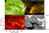 |
Fig. 1. Overview of the filament on 2020 May 25. The black rectangle in (a) outlines the field of view (FOV1) from Fig. 2, and the white rectangle outlies the field of view (FOV2) from Fig. 3. Arrows in (a)–(c) denote the brightening; (b)–(d) are overlaid with the Hα filament contour; and P and N in (d) are two magnetic patches with opposite polarities. |
Through checking the Hα images within FOV1, we find that, in the southeast of the filament, two chromospheric fibrils (“L1” and “L2”) were clearly observed at 01:41:15 UT (Fig. 2a1). Furthermore, L1 and L2 interacted with each other and almost 3 min later, a new long fibril “F1” was formed (Fig. 2a2), which moved northward and lasted about 1.5 min, and then it merged into the filament (see animation1). Between 01:44:13 UT and 01:44:57 UT, F1 moved with a projected velocity of 11 km s−1, and from 01:44:57 UT to 01:45:41 UT, the projected velocity was 14 km s−1 (Fig. 2a3). We also notice that, at the late phase of the merging, the filament main body (see the black rectangle in Fig. 2b1) became darker. Figure 2d displayed the emission variation of the filament in the black rectangular region. There was a decreasing trend of the light curve from 01:41 UT, implying the material accumulated within the filament. In other words, the mergence of the newly formed fibril into the filament supplied excess filament material and resulted in abundant absorption in the Hα image.
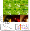 |
Fig. 2. Observations of the fibril mergence and bright sheet-like structures nearby the interaction region. (a1)–(a3): interaction of two groups of chromospheric fibrils (L1 and L2) and the subsequent formation of a northward-moving longer fibril (F1). Red and blue contours in (a1) mark a pair of magnetic patches saturated in ±50 G, where L1 and L2 are rooted. Two arrows in (a2) and (a3) denote the moving direction of F1. (b1)–(b3): similar process as that in (a1)–(a3). The black rectangle in (b2) denotes a bright sheet-like structure. The blue curve in (b3) shows the evolution of the flux of N. (c1)–(c3): bright sheet-like structure in the 171 Å, 304 Å, and 193 Å channels, respectively. (d): light curve of the filament main body (the rectangle region in (b1)). (e): light curves of the interaction region (the rectangle region in (c1)) in different channels. An animation of this figure is available online. |
In the same region, two other sets of loops (“L3” and “L4”) approached again at 01:47:54 UT (Fig. 2b1). At 01:53:04 UT, L3 and L4 interacted with each other, and a bright sheet-like structure appeared, with a length “AB” of about 3000 km and a thickness “CD” of 400 km (Fig. 2b2). Meanwhile, a new fibril “F2” was formed. By checking the EUV images from SDO, we find that the sheet-like structure observed in the Hα images has a corresponding bright structure in EUV channels (see Figs. 2c1–c3). The light curves of the sheet-like structure (the region outlined by a white rectangle in Fig. 2c1) are shown in Fig. 2e. From 01:41 UT, the brightenings increased rapidly in several minutes. For the EUV channels (304 Å, 193 Å and 171 Å), the brightenings reached the peak between 01:52 UT and 01:56 UT (the yellow ribbon).
In order to understand the photospheric magnetic field environment relevant to these interacting chromospheric fibrils, we examined the HMI line-of-sight magnetograms from 23:15 UT on May 24 to 03:14 UT on May 25. There was a pair of opposite-polarity magnetic patches in the southeast of the filament. The positive patch is named P, and the negative one is named N (see Figs. 2a1, b1, and b3). The interacting chromospheric fibrils are anchored in P and N (Figs. 2a1 and b1), respectively. Since 01:41 UT, magnetic patch N exhibited a decreasing trend (see Fig. 2b3). At 01:57 UT, its magnetic flux was −0.6 × 10¹⁸ Mx, which is almost a quarter of that (−2.4 × 10¹⁸ Mx) at 01:41 UT, implying that a continuous magnetic cancellation took place during that period.
Following the merging of new chromospheric fibrils into the filament, the original filament fibrils were detected to be disturbed. The newly formed F1 merged into the filament around 01:44 UT, and a disturbance of “f1” was subsequently observed around 01:47 UT. From 01:47:10 UT to 01:50:17 UT, f1 moved northward with a projected velocity of 5 km s−1 (Fig. 3a3, see the left panel of animation2). Similarly, F2 merged into the filament near 01:53 UT, then f2 was disturbed. From 01:55:17 UT to 01:56:45 UT, f2 moved northward with a projected speed of about 3 km s−1, and between 01:56:45 UT and 01:58:58 UT, it was about 5 km s−1 (Fig. 3b3, see the right panel of animation2).
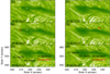 |
Fig. 3. Evidence of filament fibril disturbances. The dotted curves in (a1)–(a3) outline a filament fibril f1 which moves northward. The different color curves represent the same fibril at a different time, and the arrows in (a1) and (a2) denote the moving direction. The Hα images in (b1)–(b3) show a similar process as that in (a1)–(a3), but for another fibril, f2. An animation of this figure is available online. |
4. Summary and discussion
Based on high spatial resolution Hα and SDO observations, we display for the first time that chromospheric fibrils merge into a filament. Two sets of chromospheric fibrils which root in a pair of opposite-polarity magnetic patches interact with each other, with weak brightenings at the interacting region. Then a new chromospheric fibril is formed, moves northward, and finally merges into a nearby filament. Subsequently, the filament is disturbed, manifesting as some filament fibrils moving northward.
There is no doubt that magnetic reconnection plays a key role in the formation of filaments (Yan et al. 2015) and the eruption of filaments (Moon et al. 2007; Joshi et al. 2016; Yang et al. 2020; Hou et al. 2020). According to the magnetic reconnection theories, evident reconnection signatures include the rearrangement of magnetic field topology, the current sheet, and plasma ejection (Furth et al. 1963; Kopp & Pneuman 1976; Tsuneta 1996; Xue et al. 2018). In this work, we suggest that magnetic reconnection works in the formation of the new chromospheric fibrils. Observations that the arrangement of fibrils changed from vertical to horizontal relative to the main axis of the filament (Fig. 2) is in agreement with the signals that magnetic reconnection theories predicted, that is, magnetic topology change (Petschek 1964). With the development of the observation facility, Yang et al. (2015) found a current sheet during the small-scale magnetic reconnection, with a length and thickness about 1400 km and 420 km. In our work, the length and thickness of the bright sheet-like structure observed in Fig. 2 were about 3000 km and 400 km, similar to that of Yang et al. This bright sheet-like structure is very consistent with the radiation structure of the current sheet in small-scale magnetic reconnection (Chen et al. 2019; Xue et al. 2021).
After formed by the reconnection mentioned above, the long fibril F1 was observed to merge into the surrounding filament (see Fig. 2). However, since the true structures of the solar atmosphere are three-dimensional while the observational images are two-dimensional, the projection effect should be taken into account when we discuss the dynamical evolution of F1. As a result, the truth of the merging process ought to be considered carefully. If the merging is true, we speculate that the filament should be disturbed in some way. Fortunately, the disturbing signal was recorded by Hα images. After F1 merging into the filament, some of the original filament fibrils, for example, f1 in Figs. 3a1–a3, moved northward. Another disturbance took place several minutes later (see Figs. 3b1–b3). These pieces of observational evidence support the idea that the new chromospheric fibrils are indeed merging into the filament.
To illustrate the merging process, several schematic drawings are displayed in Fig. 4. Chromospheric fibrils L1 and L2 are rooted in a pair of opposite-polarity magnetic patches P and N, respectively. The magnetic reconnection between L1 and L2 produces the new chromospheric fibril F1. F1 moves northward and finally merges with the filament. The mergence leads to the disturbance of the filament, manifesting as the northward motion of filament fibril f1.
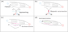 |
Fig. 4. Schematic drawings illustrating the merging process. (a): two chromospheric fibrils (L1 and L2) near a filament rooted in a pair of opposite-polarity magnetic patches with a P and N approach. (b): magnetic reconnection (denoted by a red star) happens. (c): a new fibril F1 formed by the magnetic reconnection moving to the filament. (d): f1 moving northward. Vertical arrows in (c) and (d) denote the moving direction of these fibrils. |
The process of chromospheric fibrils merging into the filament is solid evidence that the mass of a filament can be uploaded from the chromosphere. Compared with Zou et al. (2016) and Wang et al. (2019) who reported that material was injected into the filament through magnetic cancellation in the photosphere, the material supplied in our work in some way is more similar to the levitation model: material emerges into the high atmosphere with the rising magnetic structure (Oliver et al. 1999; Kubo & Shimizu 2007). In addition to the material supply, the magnetic flux in the chromosphere also supplies into the filament magnetic system. We suggest that chromospheric fibrils can provide material and magnetic flux for a filament system by magnetic reconnection, and such observations with high resolution are unique and rare.
It is worth noting that the relationship between magnetic flux cancellation and filament formation was introduced by Martin (1998). However, due to the limitation of the previous observation condition, how the cancellation motivates the development and evolution of the filament is still unknown. Based on the high-resolution observations from NVST and SDO, the new work here shows in detail that magnetic reconnection between chromospheric fibrils could contribute to the formation of the new chromospheric fibrils and the evolution of the nearby filament (at least for the case reported here). Such details are likely beyond the capabilities of those earlier studies. Further studies will be required to see how general the processes observed here might be in various filaments.
Movies
Movie 1 associated with Fig. 2 (animation1) Access Supplementary Material
Movie 1 associated with Fig. 3 (animation2) Access Supplementary Material
Acknowledgments
We are grateful to the referee for the valuable suggestions. The observations used in this paper were obtained from the NVST and SDO. This work is supported by the National Key R&D Program of China (2019YFA0405000), the National Natural Science Foundation of China (12073001, 11790304, 11790300, and 11903050), Anhui Project (Z010118169), the NAOC Nebula Talents Program, the Youth Innovation Promotion Association of CAS(2017078), the Strategic Priority Research Program of the Chinese Academy of Sciences (XDB41000000), and the open topic of the Key Laboratory of Solar Activities of the Chinese Academy of Sciences (KLSA202116).
References
- Antiochos, S. K., MacNeice, P. J., & Spicer, D. S. 2000, ApJ, 536, 494 [NASA ADS] [CrossRef] [Google Scholar]
- Chae, J. 2003, ApJ, 584, 1084 [NASA ADS] [CrossRef] [Google Scholar]
- Chae, J., Wang, H., Qiu, J., et al. 2001, ApJ, 560, 476 [Google Scholar]
- Chen, H., Yang, J., Duan, Y., & Ji, K. 2019, ApJ, 879, 74 [NASA ADS] [CrossRef] [Google Scholar]
- Chen, P.-F., Xu, A.-A., & Ding, M.-D. 2020, Res. Astron. Astrophys., 20, 166 [Google Scholar]
- Furth, H. P., Killeen, J., & Rosenbluth, M. N. 1963, Phys. Fluids, 6, 459 [Google Scholar]
- Gaizauskas, V. 1998, in IAU Colloq. 167: New Perspectives on Solar Prominences, eds. D. F. Webb, B. Schmieder, & D. M. Rust, ASP Conf. Ser., 150, 257 [NASA ADS] [Google Scholar]
- Gaizauskas, V., Zirker, J. B., Sweetland, C., & Kovacs, A. 1997, ApJ, 479, 448 [NASA ADS] [CrossRef] [Google Scholar]
- Hirayama, T. 1985, Sol. Phys., 100, 415 [NASA ADS] [CrossRef] [Google Scholar]
- Hou, Y. J., Li, T., Song, Z. P., & Zhang, J. 2020, A&A, 640, A101 [NASA ADS] [CrossRef] [EDP Sciences] [Google Scholar]
- Huang, C. J., Guo, J. H., Ni, Y. W., Xu, A. A., & Chen, P. F. 2021, ApJ, 913, L8 [CrossRef] [Google Scholar]
- Joshi, N. C., Schmieder, B., Magara, T., Guo, Y., & Aulanier, G. 2016, ApJ, 820, 126 [NASA ADS] [CrossRef] [Google Scholar]
- Kaneko, T., & Yokoyama, T. 2017, ApJ, 845, 12 [Google Scholar]
- Kippenhahn, R., & Schlüter, A. 1957, Z. Astrophys., 43, 36 [Google Scholar]
- Kopp, R. A., & Pneuman, G. W. 1976, Sol. Phys., 50, 85 [Google Scholar]
- Kubo, M., & Shimizu, T. 2007, ApJ, 671, 990 [NASA ADS] [CrossRef] [Google Scholar]
- Kuperus, M., & Raadu, M. A. 1974, A&A, 31, 189 [NASA ADS] [Google Scholar]
- Lemen, J. R., Title, A. M., Akin, D. J., et al. 2012, Sol. Phys., 275, 17 [Google Scholar]
- Lites, B. W. 2005, ApJ, 622, 1275 [NASA ADS] [CrossRef] [Google Scholar]
- Liu, Z., Xu, J., Gu, B.-Z., et al. 2014, Res. Astron. Astrophys., 14, 705 [Google Scholar]
- Mackay, D. H., Karpen, J. T., Ballester, J. L., Schmieder, B., & Aulanier, G. 2010, Space Sci. Rev., 151, 333 [Google Scholar]
- Martin, S. F. 1998, Sol. Phys., 182, 107 [Google Scholar]
- Moon, Y. J., Chae, J., & Park, Y. D. 2007, in New Solar Physics with Solar-B Mission, eds. K. Shibata, S. Nagata, & T. Sakurai, ASP Conf. Ser., 369, 425 [NASA ADS] [Google Scholar]
- Okamoto, T. J., Tsuneta, S., Lites, B. W., et al. 2009, ApJ, 697, 913 [NASA ADS] [CrossRef] [Google Scholar]
- Oliver, R., Čadež, V. M., Carbonell, M., & Ballester, J. L. 1999, A&A, 351, 733 [Google Scholar]
- Panesar, N. K., Innes, D. E., Schmit, D. J., & Tiwari, S. K. 2014, Sol. Phys., 289, 2971 [Google Scholar]
- Panesar, N. K., Tiwari, S. K., Moore, R. L., & Sterling, A. C. 2020, ApJ, 897, L2 [NASA ADS] [CrossRef] [Google Scholar]
- Parenti, S. 2014, Liv. Rev. Sol. Phys., 11, 1 [Google Scholar]
- Pesnell, W. D., Thompson, B. J., & Chamberlin, P. C. 2012, Sol. Phys., 275, 3 [Google Scholar]
- Petschek, H. E. 1964, Magnetic Field Annihilation, 50, 425 [Google Scholar]
- Pikel’Ner, S. B. 1971, Sol. Phys., 17, 44 [CrossRef] [Google Scholar]
- Poland, A. I., & Mariska, J. T. 1986, Sol. Phys., 104, 303 [NASA ADS] [CrossRef] [Google Scholar]
- Rust, D. M., & Kumar, A. 1994, Sol. Phys., 155, 69 [NASA ADS] [CrossRef] [Google Scholar]
- Saito, K., & Tandberg-Hanssen, E. 1973, Sol. Phys., 31, 105 [Google Scholar]
- Scherrer, P. H., Schou, J., Bush, R. I., et al. 2012, Sol. Phys., 275, 207 [Google Scholar]
- Tsuneta, S. 1996, ApJ, 456, 840 [NASA ADS] [CrossRef] [Google Scholar]
- van Ballegooijen, A. A., & Martens, P. C. H. 1989, ApJ, 343, 971 [Google Scholar]
- van Ballegooijen, A. A., Cartledge, N. P., & Priest, E. R. 1998, ApJ, 501, 866 [Google Scholar]
- Wang, Y. M., & Muglach, K. 2007, ApJ, 666, 1284 [NASA ADS] [CrossRef] [Google Scholar]
- Wang, J., Yan, X., Guo, Q., et al. 2019, MNRAS, 488, 3794 [CrossRef] [Google Scholar]
- Wei, H., Huang, Z., Hou, Z., et al. 2020, MNRAS, 498, L104 [NASA ADS] [CrossRef] [Google Scholar]
- Xue, Z., Yan, X., Yang, L., et al. 2018, ApJ, 858, L4 [Google Scholar]
- Xue, Z. K., Yan, X. L., Yang, L. H., et al. 2021, ApJ, 915, 17 [NASA ADS] [CrossRef] [Google Scholar]
- Yan, X. L., Xue, Z. K., Pan, G. M., et al. 2015, ApJS, 219, 17 [Google Scholar]
- Yang, S., Zhang, J., & Xiang, Y. 2015, ApJ, 798, L11 [Google Scholar]
- Yang, J., Hong, J., Li, H., & Jiang, Y. 2020, ApJ, 900, 158 [NASA ADS] [CrossRef] [Google Scholar]
- Zou, P., Fang, C., Chen, P. F., et al. 2016, ApJ, 831, 123 [NASA ADS] [CrossRef] [Google Scholar]
All Figures
|
Fig. 1. Overview of the filament on 2020 May 25. The black rectangle in (a) outlines the field of view (FOV1) from Fig. 2, and the white rectangle outlies the field of view (FOV2) from Fig. 3. Arrows in (a)–(c) denote the brightening; (b)–(d) are overlaid with the Hα filament contour; and P and N in (d) are two magnetic patches with opposite polarities. |
| In the text | |
|
Fig. 2. Observations of the fibril mergence and bright sheet-like structures nearby the interaction region. (a1)–(a3): interaction of two groups of chromospheric fibrils (L1 and L2) and the subsequent formation of a northward-moving longer fibril (F1). Red and blue contours in (a1) mark a pair of magnetic patches saturated in ±50 G, where L1 and L2 are rooted. Two arrows in (a2) and (a3) denote the moving direction of F1. (b1)–(b3): similar process as that in (a1)–(a3). The black rectangle in (b2) denotes a bright sheet-like structure. The blue curve in (b3) shows the evolution of the flux of N. (c1)–(c3): bright sheet-like structure in the 171 Å, 304 Å, and 193 Å channels, respectively. (d): light curve of the filament main body (the rectangle region in (b1)). (e): light curves of the interaction region (the rectangle region in (c1)) in different channels. An animation of this figure is available online. |
| In the text | |
|
Fig. 3. Evidence of filament fibril disturbances. The dotted curves in (a1)–(a3) outline a filament fibril f1 which moves northward. The different color curves represent the same fibril at a different time, and the arrows in (a1) and (a2) denote the moving direction. The Hα images in (b1)–(b3) show a similar process as that in (a1)–(a3), but for another fibril, f2. An animation of this figure is available online. |
| In the text | |
|
Fig. 4. Schematic drawings illustrating the merging process. (a): two chromospheric fibrils (L1 and L2) near a filament rooted in a pair of opposite-polarity magnetic patches with a P and N approach. (b): magnetic reconnection (denoted by a red star) happens. (c): a new fibril F1 formed by the magnetic reconnection moving to the filament. (d): f1 moving northward. Vertical arrows in (c) and (d) denote the moving direction of these fibrils. |
| In the text | |
Current usage metrics show cumulative count of Article Views (full-text article views including HTML views, PDF and ePub downloads, according to the available data) and Abstracts Views on Vision4Press platform.
Data correspond to usage on the plateform after 2015. The current usage metrics is available 48-96 hours after online publication and is updated daily on week days.
Initial download of the metrics may take a while.