| Issue |
A&A
Volume 658, February 2022
|
|
|---|---|---|
| Article Number | A105 | |
| Number of page(s) | 14 | |
| Section | Stellar atmospheres | |
| DOI | https://doi.org/10.1051/0004-6361/202142124 | |
| Published online | 09 February 2022 | |
A rare phosphorus-rich star in an eclipsing binary from TESS
1
Tartu Observatory, University of Tartu, Observatooriumi 1,
Tõravere
61602, Estonia
e-mail: colin.folsom@ut.ee
2
Department of Physics & Space Science, Royal Military College of Canada, PO Box 17000 Station Forces, Kingston, ON K7K 0C6, Canada
3
Department of Physics and Astronomy, University College London, Gower Street, London WC1E 6BT, UK
Received:
31
August
2021
Accepted:
8
November
2021
Context. Few exoplanets around hot stars with radiative envelopes have been discovered, although new observations from the TESS mission are improving this. Stars with radiative envelopes have little mixing at their surface, and thus their surface abundances provide a sensitive test case for a variety of processes, including potentially star–planet interactions. Atomic diffusion is particularly important in these envelopes, producing chemically peculiar objects such as Am and HgMn stars.
Aims. An exoplanet candidate around the B6 star HD 235349 was identified by TESS. Here we determine the nature of this transiting object and identify possible chemical peculiarities in the star.
Methods. HD 235349 was observed using the long-slit spectrograph at Tartu Observatory, as well as photometrically by the TESS mission. The spectra were modeled to determine stellar parameters and chemical abundances. The photometric light curve was then analyzed in the context of the stellar parameters to determine properties of the transiting object.
Results. We find the transiting object is a low-mass stellar companion, not a planet. However, the primary of this eclipsing binary is a rare type of chemically peculiar star. A strong overabundance of P is found with overabundances of Ne and Nd and mild overabundances of Ti and Mn, while He is mildly underabundant. There is also clear evidence for vertical stratification of P in the atmosphere of the star. The lack of Hg and the weak Mn overabundance suggests that this is not a typical HgMn star. It may be in the class of helium-weak phosphorus-gallium (He-weak PGa) stars or an intermediate between these two classes.
Conclusions. We show that HD 235349 is a rare type of chemically peculiar star (He-weak PGa) in an eclipsing binary system with a low-mass stellar companion. This appears to be the first He-weak PGa star discovered in an eclipsing binary.
Key words: stars: individual: HD 235349 / stars: abundances / stars: chemically peculiar / binaries: eclipsing / planets and satellites: detection / ephemerides
© ESO 2022
1 Introduction
The Transiting Exoplanet Survey Satellite (TESS) mission (Ricker et al. 2015) recently identified HD 235349 (TOI 1356.01, TIC 277566483, αJ2000 = 20h44m46s.7, δJ2000 = +54°30′07″.86) as an object of interest based on photometric transits. The TESS light curve of HD 235349 contains a periodic transit signature with a depth of 0.75% and a period of 24.28546 ± 0.00102 days, as reported in the Exoplanet Follow-up Observing Program for TESS (ExoFOP-TESS)1 database (and later confirmed by our own inspection of transit times). Based on discrepant previous effective temperature values, the star may be among the hottest exoplanet hosts to date or, alternatively, the large primary of an eclipsing binary. In order to clarify its nature, we carried out a comprehensive analysis of HD 235349, including a detailed chemical composition determination and a radial velocity time series.
HD 235349 is an early-type star with a Gaia Early Data Release 3 (EDR3) parallax distance of d = 1901 ± 180 pc (Bailer-Jones et al. 2021). It was chosen as one of the first targets in the PIVOT (Planetary InitatiVe at the Observatory of Tartu) project, which is aimed at characterizing stars with exoplanets, protoplanetary disks, or chemical peculiarities. The TESS Object of Interest Catalog lists a transit depth of 0.75% and a classification of planetary candidate (PC). The two different primary star temperatures listed by the ExoFOP-TESS database place the transiting companion as either a giant planet (if Teff = 8381 ± 409 K) or a low-mass star (if Teff = 12 308 ± 144 K). These and other available Teff estimates for the primary disagree at high confidence, further motivating a follow-up analysis.
Stars with spectral type earlier than F5 (M⋆ ≥ 1.4 M⊙) are of particularinterest because, in addition to the more familiar planet-metallicity correlation (Gonzalez 1997; Fischer & Valenti 2005), causal links may exist between certain chemically peculiar early-type stars and their planetary systems (Jura 2015; Kama et al. 2015). More generally, due to the lack of a convective envelope, superficial chemical peculiarities arise in early-type stars for a variety of reasons, such as radiative levitation (Am stars; Catanzaro et al. 2019, and references therein), magnetic flotation with slow rotation (Ap/Bp; Mathys 2020), gravitational settling with slow rotation and a lack of magnetic fields (HgMn; Alecian & Michaud 1981; Makaganiuk et al. 2011), or “accretion contamination” due to a lack of strong mixing (e.g., λ Boö; Paunzen 1998).
We describe our spectroscopic observations in Sect. 2. In Sect. 3 we detail the spectral fitting, abundance analysis, and the radial velocity and photometric light curves. We present the resulting stellar composition and parameters in Sect. 4, as well as constraints on the secondary’s properties. The chemical peculiarity of HD 235349 and the nature of its secondary are discussed in Sect. 5.
Spectra of HD 235349 obtained with the 1.5 m telescope at Tartu Observatory.
2 Observations
Spectroscopic observations of HD 235349 were carried out at Tartu Observatory2 (58°15′57′′ N, 26°27′35′′ E) in Estonia with the 1.5-m Cassegrain reflector AZT-12 (see Appendix A for full details) on 11 nights from June 2020 to April 2021. A typical session included observations of radial velocity and spectrophotometric standard stars. The long-slit spectrograph ASP-32 at the Cassegrain focus was used with 1800 lines/mm and 1200 lines/mm gratings. The wavelength coverage extended from 3704Å to 7943Å with signal-to-noise ratios (S/N)from ≈70 to 200. The full list of observations is given in Table 1.
The data were processed using the IRAF3 (Tody 1986) software built-in packages for charge-coupled-device pre-processing, spectroscopy, and cross-correlation. Spectrophotometric standards (Vega and 10 Lac) from the CALSPEC database (Bohlin et al. 2020) were used to correct for the complex instrumental profiles of some observed spectra, but absolute flux calibrations were not attempted. After bias removal and flat fielding with a lamp, spectral extraction was performed using the long-slit spectrum processing routines in ctioslit and onedspec packages. Sigma spectra were used to estimate the S/N of science spectra. Thorium-argon arc lamp spectra were recorded before and after each science integration, their dispersion solutions were averaged. Heliocentric correction was carried out with the IRAF tasks rvcorrect and dopcor. Forabundance analysis, spectra were averaged nightly. The continuum was normalized by fitting a low degree cubicspline using a custom program created in Python programming language. The spectral resolution was measured using Gaussian fits to well-isolated ThAr emission lines close to the central wavelength in each spectral setup. The average Gaussian full width at half maximum was used as the width of instrumental profile of the spectrograph.
3 Analysis
3.1 Fundamental parameters based on spectroscopy
3.1.1 Balmer line analysis
Since the fundamental parameters of HD 235349 are not well constrained in the literature, we attempted to derive them from our spectroscopic observations. Balmer lines can provide strong constraints on Teff and log g. The observationsshow no sign of emission lines or infilling, and the star is cool enough that the stellar wind should not contribute substantially to the observed lines. Thus we proceeded by directly fitting model spectra to the observations.
To calculate the model spectra we used the ZEEMAN spectrum synthesis code (Landstreet 1988; Wade et al. 2001), and ATLAS9 model atmospheres (Kurucz 1993; Castelli & Kurucz 2003). Atomic line data are taken from the Vienna Atomic Line Database (VALD; Piskunov et al. 1995; Ryabchikova et al. 1997, 2015; Kupka et al. 1999).
ZEEMAN has been mostly used for metallic line analysis, particularly of magnetic and chemically peculiar stars. Since it is preferable to use one code for all the spectrum synthesis, we have added the calculation of hydrogen line profiles to the code. The hydrogen Stark broadening profiles use the grid calculated by Lemke (1997), which implements the widely used Vidal-Cooper-Smith (VCS) model of Vidal et al. (1973). Stark broadening profiles are interpolated as necessary, and are implemented for the Lyman through Brackett series, up to n = 22 of each series. Resonance self-broadening is calculated using the theory of Ali & Griem (1965, 1966), and transition data for this calculation were taken from the National Institute of Standards and Technology (NIST) Atomic Spectra Database (Kramida et al. 2020). More advanced calculations exist, and may be implemented in the future, but for the current analysis self-broadening is much weaker than Stark broadening. The broadening calculations also include thermal Doppler broadening, van der Waals broadening (with coefficients from VALD, although it is generally negligible), and microturbulence. In our implementation we use the tabulated Stark broadening profiles including thermal broadening of Lemke (1997), which is convolved with a Voigt profile that includes the other broadening terms, and then interpolated onto the wavelength grid used for the model spectrum. The model hydrogen lines here do not include the Zeeman effect, and thus are likely insufficient for strongly magnetic Ap/Bp stars, or polarized spectra, but should be sufficient for HD 235349.
To verify the accuracy of the Balmer line calculations, we tested the spectra against the Kurucz BALMER (Kurucz 1993) and SYNTHE codes (Kurucz 1993, with grids of model spectra from Munari et al. 2005 and Bertone et al. 2008), which have similar physics to ZEEMAN. This produces an excellent agreement over a wide range of temperatures, provided the same model atmospheres are used. Testing against the PHOENIX code for K-type stars (Allard et al. 2012) provides very good agreement. PHOENIX models for hotter stars (Husser et al. 2013, up to 12 000 K) provide an acceptable agreement, although these models have slightly narrower wings, which in the worst case could lead to a discrepancy in the inferred log g up to 0.1. Testing against a grid of models from PFANT (Coelho et al. 2005) provides a very good agreement, similar to SYNTHE, although this grid only extends to 8000 K. Testing against spectra from the BSTAR2006 grid of the TLUSTY code (for cooler B-type stars in the grid, Lanz & Hubeny 2007) provides excellent agreement, except for the line cores of Hα and Hβ.
In observations of Balmer lines, a very precise continuum normalization is difficult and sometimes not practically possible. To account for possible errors in the continuum placement of the observation, we include a continuum polynomial in the model spectrum for fitting Balmer lines. For this we use a simple quadratic polynomial, in the form c0 + c1λ + c2λ2. Including this significantly reduced the scatter in best-fit Teff and log g from individual Balmer lines.
In order to determine optimal Teff and log g values, and probe their probability distributions, we adopted a Markov chain Monte Carlo (MCMC) approach. This is more computationally intensive than simply fitting by χ2 minimization, but offers two advantages. First, there tends to be a covariance between Teff and log g, and MCMCallows us to characterize the correlation in their formal uncertainties. Second, while we include three coefficients for our continuum polynomial, and they will have some influence on the uncertainties of Teff and log g, we do not care about the values of those coefficients, they are effectively nuisance parameters. An MCMC approach allows us to marginalize over these parameters (in a Bayesian sense), to derive distributions of the parameters of interest. We used the EMCEE package from Foreman-Mackey et al. (2013), which uses the MCMC affine-invariant ensemble sampler of Goodman & Weare (2010). This package has the advantages of being robustly tested and easy to integrate with existing code. The integration with EMCEE was implemented as a Python wrapper around the existing Fortran code of ZEEMAN.
For this analysis we used the lower resolution observation from September 19, 2020, with λ∕Δλ = 2620, spanning 3803–4750 Å, since the resolution is sufficient for the Balmer lines and this provides Hγ through H9 in one observation. Consistent results were obtained from the higher resolution observation from the same night spanning 3933–4509 Å, covering the Hγ and Hδ lines. The results for individual lines are presented in Appendix B and Fig. B.1. To get the final values shown in Table 2, we take the median of the Teff and log g distributions for each line, and take the average over the five lines as the global best value and the standard deviation as the formal uncertainty. This standard deviation is consistent with the uncertainties on individual lines.
3.1.2 Helium and metal line analysis
In order to derive chemical abundances for a range of elements, as well as v sin i and microturbulence (vmic), we fit observations of metallic lines across most of the visible range. A secondary analysis where we derive Teff and log g from metal lines simultaneously with chemical abundances is discussed in Appendix B. Synthetic spectra were calculated with ZEEMAN, using ATLAS9 model atmospheres and atomic line data from VALD. The VALD line lists were obtained from an “extract stellar” request with enhanced abundances for peculiar elements. The hyperfine splitting (HFS) calculations in VALD from Pakhomov et al. (2019) were included in the line list. Testing with and without HFS components produced consistent results for the best-fit abundances, well within our uncertainties4.
Stellar parameters were derived by directly fitting synthetic spectra to the observations using the χ2 minimization code of Folsom et al. (2012). Since He I lines are prominent in the spectrum and in the He abundance is important, we included the Stark broadened profiles of Barnard et al. (1969, 1974, 1975) in the opacity profile calculations for the He I 4471, 4387, 4026, and 4921 Å lines.
For this analysis we used the higher resolution observations (obtained with the 1800 mm−1 grating). While the spectral resolution is not particularly high, it is still well below the rotational broadening of the star, so it is sufficient for an abundance analysis. The combination of these observations covers ~330 to ~500 Å and generally contains a good number of lines for simultaneously determining stellar parameters; thus, we fit each observation independently. Where we had multiple observations covering the same wavelength range we used the highest S/N observation. (The 7292–7943 Å observations were not used, since they contained few detectable lines of interest.) This provides us with 5 spectral windows covering 4014–4500, 4375–4742, 4910–5310, 5281–5663, and 6007–6229 Å. Balmer lines and telluric lines were excluded from these regions. While Balmer lines could be fit simultaneously with the metal lines, they would dominate the resulting χ2 (and constraints on Teff and log g); thus, we prefer to fit them separately so as to obtain an independent constraint from metal lines. Sample best-fit spectra are shown in Fig. 1.
When comparing our best-fit models to the observations, we noted a number of S II lines with discrepant line strengths. Comparing oscillator strengths for these lines from the VALD and NIST databases, we find significant differences in the theoretical value, with the NIST values rated “C” or better. Using the NIST log gf values produced more consistent results, improving the fit to the observations, and thus we adopted the NIST log gf values for S II when available. For similar reasons we adopted the NIST loggf values for the P II 5152.2 and 5191.4 Å lines and Si II 5041.0, 5055.98, and 5056.3 Å lines.
For each of the five identified spectral regions above, we fit for v sin i, vmic, and chemical abundances for any elements with detected lines. The 4014–4500 and 4375–4742 regions did not produce reliable values of vmic, and thus forthese regions we assumed the average value from the other three regions. For the elements Cr, Ga, Pr, and Hg, we do not detect any individual lines; however, they are of interest for determining the type of chemical peculiarity in a star, particularly for HgMn stars and helium-weak phosphorus-gallium (He-weak PGa) stars. Thus we used the strongest theoretically predicted line in our observed ranges to place upper limits on the elements. These limits were determined by eye, taking the largest abundance that produced a model reasonably consistent with the observation. The Hg line at 3983.9 Å is particularly interesting for this, as it is usually detected in HgMn stars, and its absence in HD 235349 (illustrated in Fig. 2) suggests this is not a typical HgMn star.
To produce the final results we take the average of the values for each spectral region, and as an uncertainty we use the standard deviation. For elements with abundances from fewer than three regions, the uncertainty was estimated by eye, accounting for the scatter between different lines, the impact of blending lines, noise in the observation, and potential normalization errors. For elements with abundances from three or more regions we verified that the standard deviation was reasonably consistent with the scatter between lines within one region and the noise in the observations. These uncertainties, from the scatter in independent fits to different spectral regions, should account for errors in the atomic line data and normalization; however, they should still be considered somewhat approximate.
Best-fit stellar parameters and chemical abundances for HD 235349.
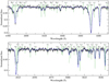 |
Fig. 1 Observed spectrum of HD 235349 obtained with the Tartu Observatory long-slit spectrograph (black, with light gray error bars) and the best-fit-model spectrum (blue). Species contributing to the stronger lines in the spectrum are indicated (green). |
3.1.3 Stratification of phosphorus
In the initial abundance analysis, we found a clear wavelength dependence in the P abundance from different spectral windows, while the other abundances and stellar parameters had no significant correlation with wavelength. This could be a hint of vertical stratification in abundance of that element, since the excitation potential of the lower level, and implicitly the depth that the line is formed at, also correlate with wavelength. To investigate this we first looked at chemical abundances derived from individual lines, and then considered a simple parametric model to improve the global fit to all lines.
In order to derive best-fit chemical abundances for individual P lines, we first adopt the best-fit stellar parameters and abundances for other elements from Table 2. We then look for P lines that are at least marginally detected above the noise and are not in a blend that is dominated by a different element. This produced 29 usable lines between 4045 and 6089 Å. Several lines of varying quality are illustrated in Fig. 3. We used the procedure of Khalack et al. (2007) to derive a proxy for the depth that each line is formed at. This takes the point in the atmosphere where the optical depth at the line center (τℓ) reaches 1. That depth is reported in terms of the optical depth in the continuum at 5000 Å (τ5000). Real lines form over a range of depths in the star, with important contributions from above τℓ = 1; however, this proxy is useful when investigating chemical stratification and looking for correlations between abundance and optical depth. To approximately account for this range of depths, we also calculated the point where τℓ = 0.1. We plot the abundance found for each line against the optical depth for that line in Fig. 4, and find a clear correlation with larger abundances for lower optical depths.
As a second approach we fit a simple parametric model for the vertical distribution of P, by calculating model spectra with this distribution and fitting them to the 29 lines identified above simultaneously. This approach requires an assumption about the functional form of the P distribution, and we considered three options. The first was a linear relation between the P abundance and logτ5000, the second was a step function with two constant abundances above and below a transition at one depth, and the third was a linear (in log τ5000) transition region with constant abundances above and below. All three options reached nearly identical, statistically consistent, χ2 values for the best-fit models. However, the second and third option require more free parameters, and those parameters became increasingly poorly constrained. Thus we conclude that we cannot place a strong constraint on the functional form of the stratified distribution,likely since many of the P lines are very near the noise level in our observations, and adopt the simplest function: a linear relation.
To explore the probability distribution of the parameters, and potentially strong co-variances, we used the same MCMC routine as was used for the Balmer lines in Sect. 3.1.1. The free parameters of the model are the abundance at τ5000 = 1 and the slope of abundance (logP∕H) with logτ5000. The results of modeling these lines are presented in Sect. 4.2, with the best-fit model in Fig. 3, showing clear support for a stratified distribution of P.
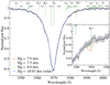 |
Fig. 2 Observed spectrum of HD 235349 (black), and model spectra varying the Hg abundance. |
3.2 Radial velocity perturbations
Our spectral observations sampled 11 individual nights over a baseline of ≈ 10 months. This allowed us to determine the radial velocity amplitude KRV of the primary and constrain the nature of the transiting companion. Radial velocity (RV) measurements were performed on the long-slit spectra using a cross-correlation approach and the IRAF task fxcor (Fitzpatrick 1994). The correlation template was a normalized R = 20 000 model spectrum from Munari et al. (2005), specifically the model in their grid closest to our derived parameters. The resulting instantaneous RV values range from − 28.5 to 7.2 km s−1 and are listed in Table 3. Fitting the RV curve with a pure sine wave and assuming zero eccentricity, we find KRV = (13.72 ± 0.63) km s−1.
3.3 Photometric light curve
TESS has observed HD 235349 (TOI 1356.01) in sectors 15 and 16, where two exoplanet transit-like events were discovered. The depth of those events is ≈ 7.5 ppt. The photometric data from the TESS data portal have strong systematic effects; therefore, we measured the target and several surrounding comparison stars from cuts of calibrated full-field TESS images using traditional aperture photometry methods. Remaining residuals in the light curve were removed by fitting with a low order cubic spline.
The ExoFOP-TESS database reports a period of 24.28546 ± 0.00102 days for these transits. Phase folding our extraction of the TESS photometry with this period, we find a good agreement in the timing of the eclipses, and thus we confirm the period reported in ExoFOP-TESS. Figure 5 shows the phase-folded TESS light curve and our radial velocity time series for HD 235349. The offset of the radial velocity curve from the transit phase curve suggests an eccentric orbit, though we caution that due to possible systematics in our long-slit spectra, stable higher S/N follow-up is necessary to test this.
4 Results
4.1 Stellar parameters
The spectroscopically determined best-fit parameters of HD 235349 are summarized in Table 2. We adopt here the values determined from the hydrogen Balmer lines: Teff= 14 757 ± 264 K and log g = 3.34 ± 0.11.
The current mass and age of HD 235349 were determined by comparing its position in an effective temperature (Teff) – surface gravity (log g) diagram with stellar evolution models without rotation at solar metallicity (Z = 0.014; Ekström et al. 2012), as shown in Fig. 6, and interpolating between models in log mass. From this, we find a stellar mass M⋆  , radius R⋆
  , and luminosity log(L⋆∕L⊙) = 3.55 ± 0.19. We adopt these as our final values. As a consistency check, empirical calibrations of M⋆ and R⋆ as polynomial functions of Teff, log g and [Fe/H] (Torres et al. 2010) give consistent results with the above numbers.
The distance to HD 235349 was recently determined to be d = 1901 ± 180 pc using the Gaia EDR3 parallax (Bailer-Jones et al. 2021). However, the current value may not be entirely reliable, since the renormalized unit weight error (RUWE) is 2.842, while “good” solutions according to the EDR3 should have a RUWE near 1.0 (or <1.4). Additionally, the EDR3 parameter “goodness of fit statistic of model wrt along-scan observations” is 38.3435, while good fits to the data should be < 3. The EDR3 parallax (0.5051 ± 0.0498 mas) is also statistically incompatible with the DR2 value (0.1530 ± 0.0834 mas). The newer EDR3 value is likely more reliable (the older value has similar quality warnings), but we consider the possibility that there is a significant systematic error in the value. Relying on the spectroscopic stellar parameters and apparent magnitude, we can compare the Gaia distance with a luminosity-based distance. We use the previously calculated log (L∕L⊙) = 3.55 ± 0.19 to obtain the stellar bolometric magnitude. Adopting a solar bolometric luminosity L⊙ = 3.828 × 1026 W and an absolute bolometric magnitude Mbol = 0 mag for a luminosity L0 = 3.0128 × 1028 W (Resolution B2 of the XXIXth International Astronomical Union General Assembly in 2015), we obtain
 (1)
(1)
Applying a bolometric correction BCV = −1.19 ± 0.04 (Pedersen et al. 2020), we find an absolute magnitude of MV = −2.95 ± 0.52 mag. The apparent magnitude is mV = 9.043 ± 0.003 mag and the reddening E(B − V) = 0.263 ± 0.050 (Stassun et al. 2019). Assuming R(V) = 3.1, we find an extinction of AV = 0.817 ± 0.156.
Using the standard relation
 (2)
(2)
where d is in parsecs, we then find that HD 235349 is d = 1721 ± 543 pc away, consistent within error bars with the distance from Gaia EDR3 determined by Bailer-Jones et al. (2021).
We further use the theoretical isochrones from Ekström et al. (2012) to determine an age log τ ≈ 7.68 ± 0.10 yr. This is also illustrated in Fig. 6. Using the corresponding evolutionary tracks, we find that on the zero-age main sequence, HD 235349 would have had Teff ≈ 21 000 K and log g ~ 4.35.
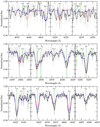 |
Fig. 3 Selection of the P lines used for the stratification analysis. The observation is shown in black (error bars in light gray), the best-fit model with a vertically constant abundance is in red, and the best-fit model with a linear variation in the abundance with log optical depth is in blue. |
Radial velocity measurements of HD 235349.
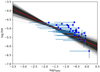 |
Fig. 4 Abundance estimates of P as a function of optical depth (τ5000). Abundances for individual lines are shown as points where the optical depth in the line center reaches unity. The horizontal bar extends to where the optical depth in the line center is 0.1 to illustrate the range of depths relevant for line formation. Vertical errors are the statistical uncertainty on the abundance. The red line is the best (median) linear P distribution from directly fitting all observed P lines simultaneously. The light gray lines represent individual models from the Markov chain, with darker gray areas corresponding to a higher probability density. |
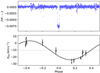 |
Fig. 5 Phased orbital variability tracers. Upper panel:phase-folded TESS light curve for HD 235349. Lower panel: Tartu Observatoryradial velocity time series (markers) overlaid with a sinusoid fit (solid line). |
4.2 Chemical abundances and stratification
The best-fit chemical abundances (see Table 2) and plotted relative to solar abundances in Fig. 7 (in log (X∕H) units). We find a strong overabundance of P by 1.48 ± 0.20 dex relative to solar, and significant overabundances of Ne by 0.65 ± 0.23 dex, and of Ti by0.66 ± 0.20 dex. Nd also appearsto be strongly overabundant, although this is less certain as it is based on a few marginally detected lines. Mn and Ni are marginally enhanced (by 0.54 ± 0.27 and 0.38 ± 0.14 dex, respectively). C, O, Mg, Al, and Fe are all consistent with solar abundances (within 2σ). He appears to be weakly depleted (− 0.25 ± 0.10 dex), although this abundance is particularly sensitive to Teff. Si also appears to be slightly depleted (−0.34 ± 0.16 dex). Thus HD 235349 is clearly chemically peculiar, although it does not display the peculiarities typical of an HgMn star, and is only a very mild, marginally He-weak star (although it does have the enhanced P common to the He-weak PGa stars).
The He abundance is particularly temperature sensitive, if our Teff were overestimated by ~500 K the He abundance would be within uncertainty of solar (see Appendix B). Alternately, if our Teff was underestimated, that could lead to a larger He underabundance. Ne I lines may show some weak nonlocal thermodynamic equilibrium (NLTE) effects in B-type stars (Alexeeva et al. 2020) (for Ne II NLTE corrections appear to be negligible). The NLTE corrections for Ne I at a Teff near 14 000 K appear to reduce the Ne abundance by a few 0.1 dex (Alexeeva et al. 2020), possibly exceeding our error bar, but unlikely to produce an abundance consistent with solar, or chemically normal B-type stars.
From analyzing individual P lines (Sect. 3.1.3) we find that lines formed mostly at smaller optical depths require significantly larger abundances of P to match the observations than lines formed deeper in the atmosphere. The individual abundances and depths where τℓ = 1 are plotted in Fig. 4, and we interpret this as evidence for stratification of P in the stellar atmosphere. From simultaneously fitting P lines with synthetic spectra in an MCMC analysis, we find a clear negative slope in abundance with log τ5000 (− 0.52 ± 0.08), and an abundance at τ5000 = 1 that is still enhanced relative to solar ( dex), with an important covariance between these two parameters. This P distribution is better constrained in the range of log τ5000 between −1 and −2, and becomes poorly constrained above logτ5000 −3 or below 0. A set of model P distributions from the final Markov chain are presented in Fig. 4 as overlapping gray lines; thus, darker regions correspond to a higher density of models and a higher probability of the parameters. The posterior probability densities of the parameters are shown in Fig. 8. From the combination of the single line analysis andthe parametric MCMC model, we find good evidence for stratification of P, with larger abundances higher in the atmosphere.However, since many lines of P are only marginally detected in our observations, higher precision data are needed before more details of the P distribution can be confidently constrained.
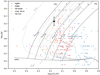 |
Fig. 6 Evolution tracks (solid lines) and isochrones (dashed lines, solid line for zero age main sequence) for nonrotating stars at Z = 0.014 from Ekström et al. (2012). Annotations give the mass at zero age main sequence for evolution tracks and the age for isochrones. The position of HD 235349 is given by the larger black point. A comparison sample of other chemically peculiar stars from Ghazaryan et al. (2018, 2019) are indicated with smaller colored points. |
4.3 Properties of the transiting secondary
The mass of the secondary star can be constrained in two ways. Firstly, using the observed transit depth (7.5 ppt) and our radius estimate for the primary, we obtain the radius of the secondary,  . In this radius estimate we assume the secondary is fully projected on the disk of the primary during photometric minimum, which is supported by the flat bottomed transits, and that the secondary contributes negligibly to the flux in the TESS band,which is supported by the small transit depth (suggesting a small cool object). In that case the ratio R2 ∕R1 is the square root of the transit depth, and the uncertainty on R2 is dominated by the uncertainty on R1. Using a main sequence mass-radius relation for low-mass stars (≤ 1.5 M⊙; Eker et al. 2018), we find a secondary mass
  . Secondly, wecan obtain M2 from the radial velocity perturbation amplitude of the primary, given by
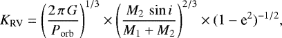 (3)
(3)
where Porb is the orbital period, e the orbital eccentricity, here assumed to be zero, i is the inclination of the orbit, here assumed to be 90°, and KRV = 13.72 ± 0.63 km s−1 (Sect. 3.2). This leads to a mass of  M⊙. If we instead assumed i = 80°, M2 would increase by only ~0.01 M⊙. If we assumed e = 0.2, that would decrease the mass by ~0.02 M⊙, and e > 0.45 would be needed to exceed our formal error bar. We summarize these constraints on M2 in Fig. 9. The results from both constraints are consistent, and point to M2 in the range 0.7–0.8 M⊙.
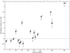 |
Fig. 7 Derived abundances relative to the solar abundances of Asplund et al. (2009). Downward pointing arrows indicate upper limitsonly. While many elements have near solar abundances, strong peculiarities are found for P, and moderate peculiarities for Ne and Ti. |
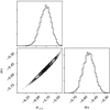 |
Fig. 8 Posterior distributions of the model parameters for a linearly stratified P abundance from the MCMC analysis. Pτ=1 represents the abundance at τ5000 = 1, while P∕τ is the slope in abundance with logτ5000. The lower left panel indicates strong covariance between these parameters. |
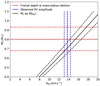 |
Fig. 9 Mass of the transiting secondary companion as a function of radial velocity perturbation on the primary. The mass of the secondary is constrained by the transit depth, using a main sequence stellar mass-radius relation (red lines), and by the radial velocity amplitude of the primary, assuming a circular Keplerian orbit (blue lines). The mathematical KRV –M2 relation is also shown, with an uncertainty range reflecting the uncertain mass of the primary (black lines). |
5 Discussion
5.1 Spectral type and effective temperature
Using a Balmer line analysis, we determined an effective temperature Teff = 14 757 ± 264 K and log g = 3.34 ± 0.11 for HD 235349. This yields a spectral type B6 III (Pecaut & Mamajek 2013). These results are consistent with the highest Teff and earliest spectral types from the wide range of past estimates. As noted earlier, the ExoFOP database lists two conflicting effective temperature values for HD 235349. The latest value, from the TESS project, is Teff = 8381 ± 409 K. In the databases listed on ViZieR5, a wider range of Teff estimates can be found, corresponding to a spectral type range from mid-A to mid-B. Spectral type classifications spanning nearly 100 yr have typically been B8 or B5 (Cannon 1927; Hill & Lynas-Gray 1977).
5.2 Chemical peculiarity
The composition of HD 235349 is clearly peculiar, with a strong overabundance of phosphorus (P, + 1.48 dex), neon (Ne, +0.65 dex), and neodymium (Nd, +1.44 dex). The upper limits for gallium and praseodymium also allow for enhancements of up to 2 dex. Furthermore, Ti, Mn, and Ni may be slightly (a factor of 0.3 to 0.6 dex) enhanced, while Si, and S appear underabundant by a similar factor and He appears to be weakly underabundant at 0.25 dex (although the He abundance is sensitive to Teff).
The star is not an obvious member of the mercury-manganese (HgMn) group of chemically peculiar stars, which extends up to temperatures similar to HD 235349 (up to ~14 000 K; e.g., Ghazaryan et al. 2018). Mn is not strongly overabundant in HD 235349, and Hg (particularly the Hg II 3984 Å line) is not detected (see Fig. 2; although the upper limit is only < 3.3 dex enhanced). Thus, the star cannot be confidently classified as an HgMn star. We compare chemical abundances for a few elements of interest, for different samples of peculiar stars6, as a function of Teff in Fig. 10. The strongest similarity between HD 235349 and HgMn-type stars is that HgMn stars are typically overabundant in P. Smith & Dworetsky (1993) and Ghazaryan et al. (2018) note a population of hot (>13 000 K) HgMn stars with mild Mn overabundances (Fig. 10), which is closer to HD 235349.
While the He abundance is only mildly below solar, the P- and potentially Ga-rich pattern is consistent with the rare class of He-weak PGa chemically peculiar stars. These are weakly or non-magnetic stars that may represent the high temperature end of HgMn stars (Borra et al. 1983). There are a few stars that have been classified as He-weak, despite apparently very modest He underabundances (e.g., Glagolevskij et al. 2007, see Fig. 10). Thus, HD 235349 has similarities to the He-weak PGa stars, although given the mild He underabundance (and sensitivity of the He abundance to Teff) we do not give it this classification with a high level of confidence.
We propose that HD 235349 represents an intermediate case between HgMn and He-weak PGa stars, perhaps with some chemical peculiarities weakened by mixing from the relatively rapid rotation of the star. There is significant evidence to support the idea that He-weak PGa stars represent a continuation of HgMn stars to higher temperatures (e.g., Borra et al. 1983; Rachkovskaya et al. 2006; Hubrig et al. 2014; Monier & Khalack 2021), with the differences in abundances due to differences in atomic diffusion with increasing temperature and perhaps an increasingly important stellar wind. HD 235349 sits near the border in Teff between these classes of objects (Ghazaryan et al. 2018, 2019), supporting the idea that it is intermediate between these classes.
Theoretical atomic diffusion calculations support this general picture. Early work by Alecian & Michaud (1981) on diffusion suggested that the overabundance of Mn in HgMn stars should fall off with increasing Teff somewhere in the Teff ~ 15 000 to 18 000 K range. HD 235349 falls on the edge of this range, and this trend is generally consistent with other observations of Mn abundances (see Fig. 10). More recent work by Alecian & Stift (2019) considers time-dependent diffusion including mass loss, with a focus on HgMn stars. They consider stratification of P, finding overabundances higher in the atmosphere, and finding that these overabundances can be greatly enhanced by a weak magnetic field.
We find clear evidence for vertical stratification in the abundance of P, with larger abundances higher in the atmosphere. This can be adequately modeled with a linear distribution of P in log τ5000, although higher S/N observations are needed to provide better constraints on the vertical distribution of P. Stratification of P, as well as someother elements, has been detected in a few HgMn stars (in HD 53929 and HD 63975 by Ndiaye et al. 2018, and in HD 161660 by Catanzaro et al. 2020) and also in HD 213781, which may be a blue horizontal branch star or an evolved HgMn star (Kafando et al. 2016). We find qualitatively consistent results with an apparently gradual increase in P abundance to shallower optical depths. This is also qualitatively consistent with the atomic diffusion models of P by Alecian & Stift (2019).
HD 235349 has a higher v sin i than is typical for an HgMn star or a He-weak PGa star. However, we are likely seeing the full equatorial rotation velocity (with i close to 90°), since the system is an eclipsing binary, and with the relatively short period the orbital and rotational axes are likely aligned. The recent survey of HgMn stars by Chojnowski et al. (2020) found an average v sini of 28 km s−1, but also 13 stars with v sin i above 60 km s−1. González et al. (2021) report a HgMn star with v sini = 124 km s−1 as the highest v sin i HgMn star yet discovered. The high v sin i of HD 235349 likely enhances mixing in the star through meridional circulation, which may reduce the amount of chemical stratification and the strength of the observed peculiarities of some elements.
We find a low log g = 3.34 ± 0.11 for HD 235349, which implies the star has likely evolved off the main sequence. However, that log g is not unprecedented among chemically peculiar stars in this temperature range, for example, the HgMn star HD 63975 (log g = 3.27, Ndiaye et al. 2018), the He-weak PGa star HD 23408 (log g = 3.3, Mon et al. 1981; Monier & Khalack 2021), and the He-weak (probably not of the PGa type) HD 5737 (log g = 3.2, Leone & Manfre 1997; Saffe & Levato 2014). The low log g may influence atomic diffusion, and contribute to the atypical pattern of chemical abundances observed, although the impact of log g on atomic diffusion is not well studied.
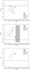 |
Fig. 10 HD 235349 in comparison to several major types of chemically peculiar early-type stars as a function of stellar Teff. Top panel:helium abundance in HD 235349 relative to the Sun, with the comparison sample from Ghazaryan et al. (2018, 2019) plotted in color. Middle and bottom panels:same as above, but for manganese and phosphorus. The gray region in the middle panel indicates the Teff range wherethe Mn enhancement should drop off toward higher temperatures (Alecian & Michaud 1981). |
5.3 Nature of the transiting object
The large radius of HD 235349 rules out a planetary explanation for the transits in the TESS light curve, instead strongly favoring a slightly subsolar mass main sequence star. Recently, it was found from speckle interferometry that HD 235349 has a close fainter (Δm = 4.1m at 832 nm) companion at the angular distance of 0.263 arcseconds (Howell et al. 2021). It is probable that HD 235349 and this close companion form a true bound stellar system, the distance determined in current work implies the separation between two stars is at least 452 ± 143 AU (for a distance of 1721 ± 543 pc), but this is too distant to be the transiting object. We rule out contamination of the photometry from a different source blended within a TESS pixel (e.g., an eclipsing binary projected near HD 235349). There is no sign of another bright star within a 21″ diameter area, and our optical spectra also contain no indications of another blended bright star. If the ~ 0.8 % dip in the summed light curve were from a different object it would require a faint binary where one component is completely covered, but this would produce a triangular transit whereas the TESS data clearly show a flat bottom. We conclude that the transiting companion must be bound to HD 235349; this assumption leads to a companion mass ≈ 0.75M⊙ (Sect. 4.3).
There are very few known eclipsing binaries among HgMn and He-weak stars, although new data from TESS are helping to change this. Binarity is often thought to be important for generating these chemically peculiar stars, by slowing rotation rates through tidal interactions, thereby allowing atomic diffusion to proceed efficiently. Despite this, there are only ten known eclipsing binaries among HgMn stars: AR Aur (HD 34364, Nordstrom & Johansen 1994; Hubrig et al. 2006; Folsom et al. 2010), TYC 455-791-1 (Strassmeier et al. 2017), V772 Cas (HD 10260, Kochukhov et al. 2021a), V680 Mon (HD 267564, Paunzen et al. 2021), HD 72208 (Wraight et al. 2011; Kochukhov et al. 2021c), and TYC 4047-570-1, HD 36892, HD 50984, HD 55776, and HD 53004 (Kochukhov et al. 2021c). Possible eclipses have been reported in HD 161701 (Wraight et al. 2011, see also González et al. 2014), and single eclipse-like events in TESS data have been reported for HD 34923 and HD 99803 (Kochukhov et al. 2021b), but more observations are needed to confirm these. The eclipsing binary HD 66051 is of interest (Niemczura et al. 2017) although it appears to contain a magnetic Bp star (Kochukhov et al. 2018), and HD 62658 was also recently discovered to contain an eclipsing magnetic Bp star (Shultz et al. 2019). We are not aware of any eclipsing binaries among the He-weak PGa stars, perhaps due to their rarity and the difficulty in firmly establishing this classification. In this context, the eclipsing binary nature of HD 235349 is an important addition to the known hot chemically peculiar stars.
6 Conclusions
We have performed a detailed analysis of HD 235349, considering its spectroscopic properties and transiting light curve, and summarize our main findings here:
- 1.
Transit-like events visible in the TESS light curve are in good agreement with eclipses by a low-mass stellar companion in a binary system, not an exoplanet. The transit depth and radius of the primary star imply a stellar radius for the transiting object of
 ;
; - 2.
Radial velocity variability was detected in the observed spectra, which varies in phase with the transit events, implying a stellar mass for the transiting object. This dynamical mass of
 M⊙ is consistent with the mass implied by the inferred radius of the transiting object;
 - 3.
Based on fitting observations with model spectra, we classify the primary as a B6 III star, with Teff = 14 757 ± 264 K and log g = 3.34 ± 0.11;
- 4.
The primary of the system is a chemically peculiar star, showing a large overabundance of phosphorus, overabundances of neon and titanium, and a weak underabundance of helium. Clear evidence for stratification of phosphorus in the atmosphere of the star was found, with larger abundances at shallower optical depths. The spectral line of Hg II at 3984.0 Å was not detected, suggesting this is not a typical HgMn star. Instead, we propose this may be an He-weak PGa star or an intermediate between the He-weak PGa stars and the HgMn stars;
- 5.
This appears to be the first star discovered with He-weak PGa characteristics in an eclipsing binary system.
Thus, while HD 235349 may not be of further interest for exoplanet studies, as a rare eclipsing binary it could be quite useful for studies of hot chemically peculiar stars.
Acknowledgements
We thank the anonymous referee for their thoughtful advice. The authors gratefully acknowledge financial support from the Estonian Ministry of Education and Research through the Estonian Research Council institutional research funding IUT40-1 and from the European Union European Regional Development Fund project KOMEET 2014-2020.4.01.16-0029. This work isbased on observations collected with the 1.5 m telescope at Tartu Observatory, Estonia, and includes data collected by the TESS mission. Funding for the TESS mission is provided by the NASA’s Science Mission Directorate. This work has also made use of the VALD database, operated at Uppsala University, the Institute of Astronomy RAS in Moscow, and the University of Vienna; the VizieR catalogue access tool CDS, Strasbourg, France (DOI: 10.26093/cds/vizier); and the Exoplanet Follow-up Observation Program website, which is operated by the California Institute of Technology, under contract with the National Aeronautics and Space Administration under the Exoplanet Exploration Program.
Appendix A Instrument parameters
The key parameters of the AZT-12 telescope at Tartu Observatory, and the long-slit spectrograph mounted there, are given in Table A.1.
Parameters of the telescope AZT-12 and the spectrograph ASP-32 at Tartu Observatory.
Appendix B Additional temperature constraints
The primary constraints on Teff and log g are from the MCMC based fit to five Balmer lines, as described in Sect. 3.1.1. Here we include plots of the posterior distributions (marginalized over the three continuum polynomial coefficients) from the MCMC analysis for each individual line in Fig. B.1. We find an important covariance between Teff and log g for all lines. Covariances between Teff or log g and the continuum parameters (not shown) are generally weak.
As a secondary analysis we derive Teff and log g from the fit to metallic lines. Since the star is chemically peculiar, these parameters must be determined simultaneously with chemical abundances, when using metal lines. This was done using the same analysis methodology as described in Sect. 3.1.2 for the metal and He lines, using the same spectral windows and line data, but including Teff and log g as additional free parameters. The resulting fits to the observations are of a comparable quality to the previous metal line analysis. The best-fit values averaged over spectral windows are in Table B.1, with uncertainties taken as the standard deviation or estimated as before for elements with abundances from fewer than three windows. This analysis provides a weaker constraint on Teff and log g than the Balmer line analysis, but the results are consistent within uncertainties. Similarly, the chemical abundances are consistent within uncertainty, but may have slightly larger systematic errors due to the larger uncertainties in Teff and log g. The most important difference in abundance is that He becomes more abundant and uncertain (with a larger scatter between windows), putting it within 1σ of the solar abundance. Thus the lower Teff from the metal line analysis suggests the star may not be He weak, but it also produces less consistent results from different He lines, suggesting it may be less reliable.
Alternate stellar parameters and abundances, based solely on metallic and He lines.
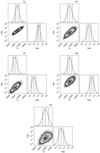 |
Fig. B.1 Posterior probability distributions of Teff and log g from the MCMC analysis of Balmer lines, after marginalizing over the continuum parameters (using corner.py; Foreman-Mackey 2016). Plots are shown for the Hγ, Hδ, Hϵ, H8, and H9 lines. Vertical dashed lines indicate the median and ± 1σ, and contoursindicate 1, 1.5, and 2σ levels. |
References
- Alecian, G., & Michaud, G. 1981, ApJ, 245, 226 [NASA ADS] [CrossRef] [Google Scholar]
- Alecian, G., & Stift, M. J. 2019, MNRAS, 482, 4519 [Google Scholar]
- Alexeeva, S., Chen, T., Ryabchikova, T., et al. 2020, ApJ, 896, 59 [NASA ADS] [CrossRef] [Google Scholar]
- Ali, A. W., & Griem, H. R. 1965, Phys. Rev., 140, 1044 [Google Scholar]
- Ali, A. W., & Griem, H. R. 1966, Phys. Rev., 144, 366 [NASA ADS] [CrossRef] [Google Scholar]
- Allard, F., Homeier, D., & Freytag, B. 2012, Phil. Trans. R. Soc. Lond. A, 370, 2765 [Google Scholar]
- Asplund, M., Grevesse, N., Sauval, A. J., & Scott, P. 2009, ARA&A, 47, 481 [NASA ADS] [CrossRef] [Google Scholar]
- Bailer-Jones, C. A. L., Rybizki, J., Fouesneau, M., Demleitner, M., & Andrae, R. 2021, AJ, 161, 147 [Google Scholar]
- Barnard, A. J., Cooper, J., & Shamey, L. J. 1969, A&A, 1, 28 [NASA ADS] [Google Scholar]
- Barnard, A. J., Cooper, J., & Smith, E. W. 1974, J. Quant. Spectr. Radiat. Transf., 14, 1025 [NASA ADS] [CrossRef] [Google Scholar]
- Barnard, A. J., Cooper, J., & Smith, E. W. 1975, J. Quant. Spectr. Radiat. Transf., 15, 429 [NASA ADS] [CrossRef] [Google Scholar]
- Bertone, E., Buzzoni, A., Chávez, M., & Rodríguez-Merino, L. H. 2008, A&A, 485, 823 [NASA ADS] [CrossRef] [EDP Sciences] [Google Scholar]
- Bohlin, R. C., Hubeny, I., & Rauch, T. 2020, AJ, 160, 21 [Google Scholar]
- Borra, E. F., Landstreet, J. D., & Thompson, I. 1983, ApJS, 53, 151 [NASA ADS] [CrossRef] [Google Scholar]
- Cannon, A. J. 1927, Ann. Harvard Coll. Observ., 100, 33 [Google Scholar]
- Castelli, F., & Kurucz, R. L. 2003, in Modelling of Stellar Atmospheres, 210, eds. N. Piskunov, W. W. Weiss, & D. F. Gray, A20 [NASA ADS] [Google Scholar]
- Catanzaro, G., Busà, I., Gangi, M., et al. 2019, MNRAS, 484, 2530 [NASA ADS] [CrossRef] [Google Scholar]
- Catanzaro, G., Giarrusso, M., Munari, M., & Leone, F. 2020, MNRAS, 499, 3720 [NASA ADS] [CrossRef] [Google Scholar]
- Chojnowski, S. D., Hubrig, S., Hasselquist, S., et al. 2020, MNRAS, 496, 832 [NASA ADS] [CrossRef] [Google Scholar]
- Coelho, P., Barbuy, B., Meléndez, J., Schiavon, R. P., & Castilho, B. V. 2005, A&A, 443, 735 [NASA ADS] [CrossRef] [EDP Sciences] [Google Scholar]
- Eker, Z., Bakış, V., Bilir, S., et al. 2018, MNRAS, 479, 5491 [NASA ADS] [CrossRef] [Google Scholar]
- Ekström, S., Georgy, C., Eggenberger, P., et al. 2012, A&A, 537, A146 [Google Scholar]
- Fischer, D. A., & Valenti, J. 2005, ApJ, 622, 1102 [NASA ADS] [CrossRef] [Google Scholar]
- Fitzpatrick, M. 1994, in ASP Conf. Ser., 61, Astronomical Data Analysis Software and Systems III, eds. D. R. Crabtree, R. J. Hanisch, & J. Barnes, 79 [Google Scholar]
- Folsom, C. P., Kochukhov, O., Wade, G. A., Silvester, J., & Bagnulo, S. 2010, MNRAS, 407, 2383 [Google Scholar]
- Folsom, C. P., Bagnulo, S., Wade, G. A., et al. 2012, MNRAS, 422, 2072 [NASA ADS] [CrossRef] [Google Scholar]
- Foreman-Mackey, D. 2016, J. Open Source Softw., 1, 24 [Google Scholar]
- Foreman-Mackey, D., Hogg, D. W., Lang, D., & Goodman, J. 2013, PASP, 125, 306 [Google Scholar]
- Ghazaryan, S., Alecian, G., & Hakobyan, A. A. 2018, MNRAS, 480, 2953 [NASA ADS] [CrossRef] [Google Scholar]
- Ghazaryan, S., Alecian, G., & Hakobyan, A. A. 2019, MNRAS, 487, 5922 [NASA ADS] [CrossRef] [Google Scholar]
- Glagolevskij, Y. V., Leushin, V. V., & Chountonov, G. A. 2007, Astrophys. Bull., 62, 319 [CrossRef] [Google Scholar]
- Gonzalez, G. 1997, MNRAS, 285, 403 [Google Scholar]
- González, J. F., Saffe, C., Castelli, F., et al. 2014, A&A, 561, A63 [NASA ADS] [CrossRef] [EDP Sciences] [Google Scholar]
- González, J. F., Nuñez, N. E., Saffe, C., et al. 2021, MNRAS, 502, 3670 [CrossRef] [Google Scholar]
- Goodman, J., & Weare, J. 2010, Commun. Appl. Math. Comput. Sci., 5, 65 [Google Scholar]
- Hill, P. W., & Lynas-Gray, A. E. 1977, MNRAS, 180, 691 [NASA ADS] [Google Scholar]
- Howell, S., Scott, N., Matson, R., et al. 2021, Front. Astron. Space Sci., 8, 635864 [Google Scholar]
- Hubrig, S., González, J. F., Savanov, I., et al. 2006, MNRAS, 371, 1953 [NASA ADS] [CrossRef] [Google Scholar]
- Hubrig, S., Castelli, F., González, J. F., et al. 2014, MNRAS, 442, 3604 [NASA ADS] [CrossRef] [Google Scholar]
- Husser, T. O., Wende-von Berg, S., Dreizler, S., et al. 2013, A&A, 553, A6 [NASA ADS] [CrossRef] [EDP Sciences] [Google Scholar]
- Jura, M. 2015, AJ, 150, 166 [NASA ADS] [CrossRef] [Google Scholar]
- Kafando, I., LeBlanc, F., & Robert, C. 2016, MNRAS, 459, 871 [NASA ADS] [CrossRef] [Google Scholar]
- Kama, M., Folsom, C. P., & Pinilla, P. 2015, A&A, 582, L10 [NASA ADS] [CrossRef] [EDP Sciences] [Google Scholar]
- Khalack, V. R., Leblanc, F., Bohlender, D., Wade, G. A., & Behr, B. B. 2007, A&A, 466, 667 [NASA ADS] [CrossRef] [EDP Sciences] [Google Scholar]
- Kochukhov, O., Johnston, C., Alecian, E., Wade, G. A., & BinaMIcS Collaboration 2018, MNRAS, 478, 1749 [NASA ADS] [CrossRef] [Google Scholar]
- Kochukhov, O., Johnston, C., Labadie-Bartz, J., et al. 2021a, MNRAS, 500, 2577 [Google Scholar]
- Kochukhov, O., Khalack, V., Kobzar, O., et al. 2021b, MNRAS, 506, 5328 [NASA ADS] [CrossRef] [Google Scholar]
- Kochukhov, O., Labadie-Bartz, J., Khalack, V., & Shultz, M. E. 2021c, MNRAS, 506, L40 [NASA ADS] [CrossRef] [Google Scholar]
- Kramida, A., Yu. Ralchenko, Reader, J., & NIST ASD Team 2020, NIST Atomic Spectra Database (ver. 5.8), [Online]. Available: https://physics.nist.gov/asd [2021, April 20]. National Institute of Standards and Technology, Gaithersburg, MD [Google Scholar]
- Kupka, F., Piskunov, N., Ryabchikova, T. A., Stempels, H. C., & Weiss, W. W. 1999, A&AS, 138, 119 [NASA ADS] [CrossRef] [EDP Sciences] [Google Scholar]
- Kurucz, R. 1993, CDROM Model Distribution, Smithsonian Astrophys. Obs. [Google Scholar]
- Landstreet, J. D. 1988, ApJ, 326, 967 [Google Scholar]
- Lanz, T., & Hubeny, I. 2007, ApJS, 169, 83 [CrossRef] [Google Scholar]
- Lemke, M. 1997, A&AS, 122, 285 [NASA ADS] [CrossRef] [EDP Sciences] [Google Scholar]
- Leone, F., & Manfre, M. 1997, A&A, 320, 257 [NASA ADS] [Google Scholar]
- Makaganiuk, V., Kochukhov, O., Piskunov, N., et al. 2011, A&A, 525, A97 [CrossRef] [EDP Sciences] [Google Scholar]
- Mathys, G. 2020, in Stellar Magnetism: A Workshop in Honour of the Career and Contributions of John D. Landstreet, eds. G. Wade, E. Alecian, D. Bohlender, & A. Sigut, 11, 35 [NASA ADS] [Google Scholar]
- Mon, M., Hirata, R., & Sadakane, K. 1981, PASJ, 33, 413 [NASA ADS] [Google Scholar]
- Monier, R., & Khalack, V. 2021, Res. Notes Am. Astron. Soc., 5, 104 [Google Scholar]
- Munari, U., Sordo, R., Castelli, F., & Zwitter, T. 2005, A&A, 442, 1127 [NASA ADS] [CrossRef] [EDP Sciences] [Google Scholar]
- Ndiaye, M. L., LeBlanc, F., & Khalack, V. 2018, MNRAS, 477, 3390 [NASA ADS] [CrossRef] [Google Scholar]
- Niemczura, E., Hümmerich, S., Castelli, F., et al. 2017, Sci. Rep., 7, 5906 [CrossRef] [Google Scholar]
- Nordstrom, B., & Johansen, K. T. 1994, A&A, 282, 787 [NASA ADS] [Google Scholar]
- Pakhomov, Y. V., Ryabchikova, T. A., & Piskunov, N. E. 2019, Astron. Rep., 63, 1010 [NASA ADS] [CrossRef] [Google Scholar]
- Paunzen, E. 1998, Contributions of the Astronomical Observatory Skalnate Pleso, 395 [Google Scholar]
- Paunzen, E., Hümmerich, S., Fedurco, M., et al. 2021, MNRAS, 504, 3749 [CrossRef] [Google Scholar]
- Pecaut, M. J., & Mamajek, E. E. 2013, ApJS, 208, 9 [Google Scholar]
- Pedersen, M. G., Escorza, A., Pápics, P. I., & Aerts, C. 2020, MNRAS, 495, 2738 [Google Scholar]
- Piskunov, N. E., Kupka, F., Ryabchikova, T. A., Weiss, W. W., & Jeffery, C. S. 1995, A&AS, 112, 525 [Google Scholar]
- Rachkovskaya, T. M., Lyubimkov, L. S., & Rostopchin, S. I. 2006, Astron. Rep., 50, 123 [NASA ADS] [CrossRef] [Google Scholar]
- Ricker, G. R., Winn, J. N., Vanderspek, R., et al. 2015, J. Astron. Telescopes Instrum. Syst., 1, 014003 [Google Scholar]
- Ryabchikova, T. A., Piskunov, N. E., Kupka, F., & Weiss, W. W. 1997, Balt. Astron., 6, 244 [NASA ADS] [Google Scholar]
- Ryabchikova, T., Piskunov, N., Kurucz, R. L., et al. 2015, Phys. Scr., 90, 054005 [Google Scholar]
- Saffe, C., & Levato, H. 2014, A&A, 562, A128 [NASA ADS] [CrossRef] [EDP Sciences] [Google Scholar]
- Shultz, M. E., Johnston, C., Labadie-Bartz, J., et al. 2019, MNRAS, 490, 4154 [NASA ADS] [CrossRef] [Google Scholar]
- Smith, K. C., & Dworetsky, M. M. 1993, A&A, 274, 335 [NASA ADS] [Google Scholar]
- Stassun, K. G., Oelkers, R. J., Paegert, M., et al. 2019, AJ, 158, 138 [Google Scholar]
- Strassmeier, K. G., Granzer, T., Mallonn, M., Weber, M., & Weingrill, J. 2017, A&A, 597, A55 [NASA ADS] [CrossRef] [EDP Sciences] [Google Scholar]
- Tody, D. 1986, SPIE Conf. Ser., 627, 733 [Google Scholar]
- Torres, G., Andersen, J., & Giménez, A. 2010, A&ARv, 18, 67 [Google Scholar]
- Vidal, C. R., Cooper, J., & Smith, E. W. 1973, ApJS, 25, 37 [NASA ADS] [CrossRef] [Google Scholar]
- Wade, G. A., Bagnulo, S., Kochukhov, O., et al. 2001, A&A, 374, 265 [NASA ADS] [CrossRef] [EDP Sciences] [Google Scholar]
- Wraight, K. T., White, G. J., Bewsher, D., & Norton, A. J. 2011, MNRAS, 416, 2477 [NASA ADS] [CrossRef] [Google Scholar]
The impact of HFS on our final results is small mostly because, at this v sin i and resolution, HFS largely has the effect of desaturating strong lines. Lines of elements with a significant nuclear dipole moment (and HFS data in VALD) are relatively weak in this spectrum, so desaturation due to HFS is very small (generally less than 1% of our uncertainties on individual pixels). However, the effect is present in lines of interest to this study (particularly Mn II and Ga II); thus, it should be included and may become significant for stars with stronger or sharper lines.
We have divided the sample of helium weak stars from Ghazaryan et al. (2019) into those with good evidence for strong magnetic fields in the literature (“mag. He-w”) and those lacking evidence for a magnetic field (“He weak”) since the presence of a strong magnetic field modifies atomic diffusion.
All Tables
Parameters of the telescope AZT-12 and the spectrograph ASP-32 at Tartu Observatory.
Alternate stellar parameters and abundances, based solely on metallic and He lines.
All Figures
|
Fig. 1 Observed spectrum of HD 235349 obtained with the Tartu Observatory long-slit spectrograph (black, with light gray error bars) and the best-fit-model spectrum (blue). Species contributing to the stronger lines in the spectrum are indicated (green). |
| In the text | |
|
Fig. 2 Observed spectrum of HD 235349 (black), and model spectra varying the Hg abundance. |
| In the text | |
|
Fig. 3 Selection of the P lines used for the stratification analysis. The observation is shown in black (error bars in light gray), the best-fit model with a vertically constant abundance is in red, and the best-fit model with a linear variation in the abundance with log optical depth is in blue. |
| In the text | |
|
Fig. 4 Abundance estimates of P as a function of optical depth (τ5000). Abundances for individual lines are shown as points where the optical depth in the line center reaches unity. The horizontal bar extends to where the optical depth in the line center is 0.1 to illustrate the range of depths relevant for line formation. Vertical errors are the statistical uncertainty on the abundance. The red line is the best (median) linear P distribution from directly fitting all observed P lines simultaneously. The light gray lines represent individual models from the Markov chain, with darker gray areas corresponding to a higher probability density. |
| In the text | |
|
Fig. 5 Phased orbital variability tracers. Upper panel:phase-folded TESS light curve for HD 235349. Lower panel: Tartu Observatoryradial velocity time series (markers) overlaid with a sinusoid fit (solid line). |
| In the text | |
|
Fig. 6 Evolution tracks (solid lines) and isochrones (dashed lines, solid line for zero age main sequence) for nonrotating stars at Z = 0.014 from Ekström et al. (2012). Annotations give the mass at zero age main sequence for evolution tracks and the age for isochrones. The position of HD 235349 is given by the larger black point. A comparison sample of other chemically peculiar stars from Ghazaryan et al. (2018, 2019) are indicated with smaller colored points. |
| In the text | |
|
Fig. 7 Derived abundances relative to the solar abundances of Asplund et al. (2009). Downward pointing arrows indicate upper limitsonly. While many elements have near solar abundances, strong peculiarities are found for P, and moderate peculiarities for Ne and Ti. |
| In the text | |
|
Fig. 8 Posterior distributions of the model parameters for a linearly stratified P abundance from the MCMC analysis. Pτ=1 represents the abundance at τ5000 = 1, while P∕τ is the slope in abundance with logτ5000. The lower left panel indicates strong covariance between these parameters. |
| In the text | |
|
Fig. 9 Mass of the transiting secondary companion as a function of radial velocity perturbation on the primary. The mass of the secondary is constrained by the transit depth, using a main sequence stellar mass-radius relation (red lines), and by the radial velocity amplitude of the primary, assuming a circular Keplerian orbit (blue lines). The mathematical KRV –M2 relation is also shown, with an uncertainty range reflecting the uncertain mass of the primary (black lines). |
| In the text | |
|
Fig. 10 HD 235349 in comparison to several major types of chemically peculiar early-type stars as a function of stellar Teff. Top panel:helium abundance in HD 235349 relative to the Sun, with the comparison sample from Ghazaryan et al. (2018, 2019) plotted in color. Middle and bottom panels:same as above, but for manganese and phosphorus. The gray region in the middle panel indicates the Teff range wherethe Mn enhancement should drop off toward higher temperatures (Alecian & Michaud 1981). |
| In the text | |
|
Fig. B.1 Posterior probability distributions of Teff and log g from the MCMC analysis of Balmer lines, after marginalizing over the continuum parameters (using corner.py; Foreman-Mackey 2016). Plots are shown for the Hγ, Hδ, Hϵ, H8, and H9 lines. Vertical dashed lines indicate the median and ± 1σ, and contoursindicate 1, 1.5, and 2σ levels. |
| In the text | |
Current usage metrics show cumulative count of Article Views (full-text article views including HTML views, PDF and ePub downloads, according to the available data) and Abstracts Views on Vision4Press platform.
Data correspond to usage on the plateform after 2015. The current usage metrics is available 48-96 hours after online publication and is updated daily on week days.
Initial download of the metrics may take a while.