| Issue |
A&A
Volume 656, December 2021
|
|
|---|---|---|
| Article Number | A51 | |
| Number of page(s) | 21 | |
| Section | Stellar structure and evolution | |
| DOI | https://doi.org/10.1051/0004-6361/202141916 | |
| Published online | 03 December 2021 | |
Planetary nebulae in Gaia EDR3: Central star identification, properties, and binarity⋆
1
Universidade da Coruña (UDC), Department of Computer Science and Information Technologies, Campus Elviña s/n, 15071 A Coruña, Spain
e-mail: iker.gonzalez@udc.es
2
CIGUS CITIC, Centre for Information and Communications Technologies Research, Universidade da Coruña, Campus de Elviña s/n, 15071 A Coruña, Spain
3
Universidade da Coruña (UDC), Department of Nautical Sciences and Marine Engineering, Paseo de Ronda 51, 15011 A Coruña, Spain
e-mail: manteiga@udc.es
4
Instituto de Astrofísica de Canarias, 38200 La Laguna, Tenerife, Spain
5
Universidad de La Laguna (ULL), Astrophysics Department, 38206 La Laguna, Tenerife, Spain
6
CSIC, Spain
7
Universidade de Vigo (UVIGO), Applied Physics Department, Campus Lagoas-Marcosende, s/n, 36310 Vigo, Spain
Received:
30
July
2021
Accepted:
24
September
2021
Context. The Gaia Early Data Release 3 (EDR3), published in December 2020, features improved photometry and astrometry compared to that published in the previous DR2 file and includes a substantially larger number of sources, of the order of 2000 million, making it a paradigm of big data astronomy. Many of the central stars of planetary nebulae (CSPNe) are inherently faint and difficult to identify within the field of the nebula itself. Gaia measurements may be relevant not only in identifying the ionising source of each nebula, but also in the study their physical and evolutionary properties.
Aims. We demonstrate how Gaia data mining can effectively help to solve the issue of central star misidentification, a problem that has plagued the field since its origin. As we did for DR2, our objective is to present a catalogue of CSPNe with astrometric and photometric information in EDR3. From that catalogue, we selected a sample of stars with high-quality astrometric parameters, on which we carried out a more accurate analysis of CSPNe properties.
Methods.GaiaGBP − GRP colours allow us to select the sources with sufficient temperatures to ionise the nebula. In order to estimate the real colour of a source, it is important to take into account interstellar extinction and, in the case of compact nebulae, nebular extinction when available. In addition, distances derived from EDR3 parallaxes (combined with consistent literature values) can be used to obtain nebular intrinsic properties from those observed. With this information, CSPNe can be plotted in an Hertzsprung-Russell diagram. From information on the spectral classification of the CS (from the literature) and evolutionary models for post-AGB stars, their evolutionary state can then be analysed. Furthermore, EDR3 high-quality astrometric data enable us to search for objects comoving with CSs in the field of each nebula by detecting sources with parallaxes and proper motions similar to those of the CS.
Results. We present a catalogue of 2035 PNe with their corresponding CS identification from among Gaia EDR3 sources. We obtain the distances for those with known parallaxes in EDR3 (1725 PNe). In addition, for a sub-sample (405 PNe) with the most accurate distances, we obtain different nebular properties such as their Galactic distribution, radius, kinematic age, and morphology. Furthermore, for a set of 74 CSPNe, we present the evolutionary state (mass and age) derived from their luminosities and effective temperatures from evolutionary models. Finally, we highlight the detection of several wide binary CSPNe through an analysis of the EDR3 astrometric parameters, and we contribute to shedding some light on the relevance of close binarity in CSPNe.
Key words: planetary nebulae: general / stars: distances / stars: evolution / Hertzsprung-Russell and C-M diagrams / binaries: general / methods: data analysis
Full Tables A.1 and A.2 are only available at the CDS via anonymous ftp to cdsarc.u-strasbg.fr (130.79.128.5) or via http://cdsarc.u-strasbg.fr/viz-bin/cat/J/A+A/656/A51
© ESO 2021
1. Introduction
This article is an extension of our previous studies on the Galactic planetary nebulae (PNe) population using Gaia Data Release 2 (DR2): González-Santamaría et al. (2019) (Paper I) and González-Santamaría et al. (2020) (Paper II). Here, we make use of the recently published Gaia Early Data Release 3 (EDR3) archive, which provides a greater quantity of higher quality astrometric and photometric data that allow us to update and enlarge our PNe catalogue and analyse its results in greater detail.
The EDR3 archive contains astrometric data (positions, parallaxes and proper motions) and photometric data (in three bands) for almost 2000 million sources with improved precision compared with DR2. These accurate new data have allowed us to carry out a study of the physical and evolutionary properties of PNe with improved statistics and to improve the reliability of nebular central star (CS) identifications. Using these data, we were also able to detect wide binary systems associated with PNe with greater precision. The Gaia mission continues its operations and will release more improved data in the near future. Specifically, the full Gaia Data Release 3 (DR3) is planned for the first half of 2022 and will contain spectrophotometry in the 330−1050 nm wavelength range for a comprehensive astronomical sample.
Recent literature entries studying the Galactic PNe population includes Weidmann et al. (2020), which provides a catalogue of 620 PNe, analysing several parameters of CSs such as spectral types, effective temperatures, and luminosities. Another study by Chornay & Walton (2020) provides a procedure for selecting central stars of planetary nebulae (CSPNe) from DR2, which was recently updated by EDR3 (Chornay & Walton 2021). Several previous studies have taken advantage of the extraordinary quality of Gaia DR2 astrometry to search for wide binaries using astrometric measurements such as that by Jiménez-Esteban et al. (2019), whose methodology was the base for the search for wide binaries among DR2 CSPNe that we presented in Paper II.
We start in Sect. 2 by explaining the procedure we used to select a sample of Galactic PNe and the method we followed to identify their CSs. As we mentioned before, the literature is plagued with CS misidentifications, and in this sense Gaia multi-band measurements are of great help in finding the source most likely to be the ionising star. From Gaia parallax measurements, we obtained distances that endorse the new Bayesian distances catalogue by Bailer-Jones et al. (2021). In Sect. 3, we select a sub-sample of PNe with the most reliable distance measurements to carry out a more detailed study of these sources. As in Paper I, we compare such distances with other measurements available in the literature that have historically been used to attribute distances and properties to PNe. Section 4 is devoted to the study of the evolutionary state of CSPNe as derived from their luminosities and effective temperatures, and to a comparison of their positions in an Hertzsprung-Russell (HR) diagram with those predicted by evolutionary tracks for post-AGB stars (Miller Bertolami 2016). This approach allowed us to estimate masses and evolutionary ages and compare their predicted evolutionary state with other properties such as size and spectral classification. Finally, in Sect. 5, we use the astrometric information available in EDR3 to look for signs of binarity among the selected CSPNe. Concretely, we search for wide binaries by using EDR3 astrometric parameters that enable us to detect objects comoving with the CSs. In addition, we carried out a statistical procedure in order to detect possible close binaries.
2. Galactic planetary nebulae catalogue
The main aim of this study is to help consolidate a Galactic CSPNe catalogue by studying the information on the properties of point-like sources present in Gaia EDR3. As in Paper I, we started by gathering as many PNe as possible from the literature. Specifically, we collected all objects catalogued as True, Likely, or Possible PNe in the HASH (Hong Kong/AAO/Strasbourg/Hα) database (Parker et al. 2016), which already contains almost all the objects listed in other PNe catalogues, such as those by Kerber et al. (2003), Stanghellini & Haywood (2010), and Weidmann et al. (2020).
In fact, we detected only 21 objects catalogued as True PNe in Weidmann et al. (2020) that are not included in HASH. If we analyse these objects, we see that they are catalogued as Symbiotic Stars, HII Regions, or Ionized ISM in HASH. We also find that these misclassifications are frequently supported by old entries in the Simbad database. Excluding these few objects, we finally gathered a total sample of 3711 PNe.
2.1. Identification of the central star in planetary nebulae
Once we collected our general PNe sample, we proceeded to search for their CSs in Gaia EDR3. We searched in the field around their nebular centre, set up by their corresponding HASH coordinates. The identification of the CS in a PN is not an easy task and has led to misidentifications that have remained unnoticed in the literature (Chornay & Walton 2020). Central stars are usually located at the geometric centre of the PN or close to it, but that is not always the case. In some instances, it is difficult to establish the geometric centre of the nebula, either because of projection effects or because of their interaction with the ISM (Villaver et al. 2012). For extended sources, there can often be several field stars around the PN centre that hinder the CS identification. The nebula itself can also contaminate the field with its brightness; this mainly happens in young and compact PNe. In these cases, the detection of the CS is even more complicated.
Apart from the distance to the nebular centre, another clue that can help to identify CSs is the colour of the star. Gaia multi-band photometry provides colours for most of the stars in the survey, and we can use, for instance, the difference between magnitudes measured by the blue photometer (BP) and the red photometer (RP), GBP − GRP, or other combinations of the G, GBP, and GRP bands to define the colour of a source. As we know, the CSPNe must have a minimum temperature to be able to ionise the nebula. As can be seen in Suárez et al. (2006), an A0-type star can give rise to the photoionisation of hydrogen, so we can assume a minimum stellar temperature of 13 000 K for a transition stage from a preplanetary nebulae (Weidmann et al. 2020) to about 25 000 K for a complete ionisation of the nebula (Kwok 2000). We can use the relationship between GaiaGBP − GRP and effective temperature obtained in Andrae et al. (2018) for a reference sample of stars with DR2 photometry to set an upper limit on the colour of the ionising source to GBP − GRP = −0.2, which corresponds to a temperature of around 13 000 K (see Fig. 3 of Andrae et al. 2018).
Interstellar reddening must be accounted for with regard to the colour of the stars, bearing in mind that we are talking about a population of stars mainly from the Galactic disc. In order to quantify and correct for interstellar extinction, we made use of the Bayestar (Green et al. 2019) and SFD (Schlegel et al. 1998) dustmaps1. We obtained the interstellar extinction for all our CS candidates by implementing a Python script to query these two databases. The idea is to correct for extinction before carrying out the search procedure for the most probable CS. This extinction distribution (up to a limit of 8 mag) in the visible band is shown in Fig. 1. Using the relations of Danielski et al. (2018), we then obtained the extinctions in the GaiaG, GBP, GRP passbands. Finally, we corrected the (GBP − GRP) colours with the corresponding extinction values.
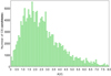 |
Fig. 1. Interstellar extinction distribution for all CS candidates. Obtained from Bayestar and SFD dust maps. |
We next considered both the distance to the nebular geometric centre (from the HASH catalogue) and the Gaia de-reddened colour (GBP − GRP)° to identify the most probable CS in the field of each PN. In carrying out this task, we considered all EDR3 sources within a radius of 20 arcsec around each of the nebular centres and obtained, on average, 40–45 candidate objects per nebula (more than 160 000 sources in total).
In order to analyse the sources present in each field and decide upon the one that was most probably the CS, we implemented an algorithm that allows us to take into account both the de-reddened colours (c) and the distances to the nebular centre (d). We first checked whether there was any star with a (GBP − GRP)° colour lower than −0.2 (the colour limit for at least partial hydrogen ionisation) inside a region close enough to the nebular centre (defined as a circular region with a radius less than the 20% of the corresponding nebular radius). If we detected more than one source within this region, we selected the one closest to the geometrical centre.
When no star was detected fulfilling these colour and distance thresholds, we built a function containing both the value of the angular distance and the colour that allowed us to select the source with the lowest value for both parameters (the closest and the bluest star). There were numerous cases where a red CSPN was detected, well above the indicated colour limit. Among the factors that could explain this type of selection was the possibility that it corresponded to a binary system where only the red companion was detected by Gaia, that the extinction correction was insufficient, or even that it was a false identification or the true CS was too weak or had a colour not measured by Gaia.
The possible values for c and d need to be normalised somehow (N(c), N(d)) in order properly to consider these two parameters (distance, d, and colour, c) of such different natures within the same function. As the CS needed to be located inside its nebula, we only considered those sources with a distance to the nebular centre below their corresponding nebular radius (R). We then normalised their distances to the interval [0,1]. In the case of sources located farther than their nebular radius, we assigned them a value of infinity in order to discard them with ease. We defined N(d) as follows:
![$$ \begin{aligned} N(d) = \left\{ \begin{array}{ll} \dfrac{d}{R},&d \in [0,R] \Rightarrow [0,1]; \\ \infty ,&d > R. \\ \end{array}\right. \end{aligned} $$](/articles/aa/full_html/2021/12/aa41916-21/aa41916-21-eq1.gif)
In a few cases in which the nebular size was unknown, we imposed a minimum radius value of 1 arcsec. If we did not find any source in this region, we did not assign a CS to that PN.
We also normalized the colour, N(c), in the [0,1] interval. From our previous study in Paper I, we know that most colours move between the values of −3 and 3. For stars with (GBP − GRP)° in this range, we scaled their colours to the ![$ [0,\frac{1}{2}] $](/articles/aa/full_html/2021/12/aa41916-21/aa41916-21-eq2.gif) interval, which corresponds to the most suitable region, whereas for stars with higher colour values (up to 4.82 in the whole sample) we scale the colour to the interval
interval, which corresponds to the most suitable region, whereas for stars with higher colour values (up to 4.82 in the whole sample) we scale the colour to the interval ![$ [\frac{1}{2},1] $](/articles/aa/full_html/2021/12/aa41916-21/aa41916-21-eq3.gif) , which was defined as the less suitable region. Finally, for the few stars with very blue colours, (GBP − GRP)° below −3, we assigned an N(c) value of 0, since we consider these to be sources with a high probability of being the ionising star. We thus obtain the following normalised value range for the colour:
, which was defined as the less suitable region. Finally, for the few stars with very blue colours, (GBP − GRP)° below −3, we assigned an N(c) value of 0, since we consider these to be sources with a high probability of being the ionising star. We thus obtain the following normalised value range for the colour:
![$$ \begin{aligned} N(c) = \left\{ \begin{array}{ll} \dfrac{3+c}{12},&c \in [-3,3] \Rightarrow [0,\frac{1}{2}], \\ 0.5 + \dfrac{c-3}{3.64},&c \in (3,4.82] \Rightarrow [\frac{1}{2},1], \\ 0,&c < -3. \\ \end{array}\right. \end{aligned} $$](/articles/aa/full_html/2021/12/aa41916-21/aa41916-21-eq4.gif)
To those objects without measured colour values, we assigned the mean colour value of all candidates, c equal to 0.775. Once both the N(c) and N(d) factors were calculated, we summed these to construct the function to be minimized in order to determine the star most likely to be the CS:

We note that this function takes values in the [0,2] interval. The source that minimises this function for each of the remaining PNe in our sample is identified as the most likely CS.
After running this algorithm, we obtained CS identifications for a total of 3257 PNe. If we compare our identifications with those of Chornay & Walton (2021), we obtain a coincidence rate of 96% within the PNe in common in both samples. We note that our algorithm considers colours already corrected for extinction, a fact that the algorithm of Chornay & Walton (2021) does not take into account. This may be the main explanation for the small mismatch.
By analysing the few differences in the CS identification between both methods (78 cases), we see that our algorithm gives slightly more priority to colours than the Chornay & Walton (2021) algorithm. Concretely, when both identifications correspond to objects with colours measured by Gaia, in more than 60% of cases our source is bluer than the one identified by Chornay & Walton (2021). In addition, when any of the identifications lacks Gaia colour, in around 55% of cases our source is closer to nebular centre than the other source.
In order to provide the community with an index indicating how reliable these identifications might be, we decided to divide the identifications into three groups (A, B, and C), in decreasing order of reliability. Stars included in group A all have colours below −0.2 and are located within 20% of the nebular radius: these sources are very likely to be CSs. Group B contains stars with values of f(c, d)≤0.5, and group C contains all the other stars. In group C, we also included those stars selected as CSs without known colours, as they are uncertain identifications.
Figure 2 shows, divided in these three groups, the stars proposed as CSs in a colour versus distance diagram, where in this case distances are calculated relative to the nebular mean radii. Of the total of 3257 identified CSPNe, 31.6% are included in group A, 30.9% in group B, and 37.5 % in group C. As the CS identifications in group C are not sufficiently reliable, we decided not to include them in our CSPNe catalogue. Consequently, our catalogue provides information for a total of 2035 CSPNe, corresponding to groups A and B.
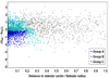 |
Fig. 2. (GBP − GRP)° colour versus relative distance to the nebular centre for those stars proposed as CSPNe. The objects are divided in three groups (A, B, and C) according to the reliability of their identification. |
In Table A.1 we list information on the Gaia EDR3 sources identified as the CS of each of these PNe. Apart from their coordinates (RA, Dec) and reliability group (quality label), several other parameters are provided, such as the angular distance to the nebular centre (Dang), the Gaia magnitudes and colours (G, (GBP − GRP), (GBP − GRP)°), and the interstellar extinction (AV). The full table is available online at the CDS.
2.2. Distances to planetary nebulae
Gaia EDR3 provides parallaxes for approximately 81% of its sources. In our catalogue of 2035 CSPNe, there are 1725 objects with EDR3 parallaxes. From these parallaxes, we can derive their distances, as we did in our Gaia DR2 study (Paper I), using the new catalogue of Bayesian statistical distances of Bailer-Jones et al. (2021). In comparison with our previous work, we have been able to estimate distances to about 10% more PNe. With DR2, we obtained distances for 1571 PNe, whereas we now have this parameter for 1725 nebulae. However, the main improvements are that the new distance determinations are more reliable than previous ones and that they come from more accurately selected CSs.
In Fig. 3, we show the obtained heliocentric distance distribution. Its peak is located around 5 kpc and about 6% of our proposed CSs are located at a distance of less than 1 kpc, while only about 1% are beyond 10 kpc.
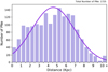 |
Fig. 3. Distance distribution of the general sample of 1725 PNe. |
If we fit a Gaussian function to this distribution, we obtain a mean value of 4.57 kpc, with a standard deviation of 2.35 kpc. This means that, in comparison with our results in Paper I (mean distance of 3.55 kpc and standard deviation of 1.94 kpc), we detect more distant and more equally distributed PNe.
3. Catalogue of CSPNe with reliable distances: GAPN-EDR3
As seen in the previous section, we were able to extract the parallaxes and, consequently, distances for a wide sample of CSPNe. Nevertheless, these parallaxes may have quite large uncertainties that translate into large distance uncertainties. In order to carry out a detailed study of the PNe, we selected only those objects with the most reliable distances.
At this point, it is important to note that parallaxes (w) in Gaia EDR3 (as was also the case for DR2 parallaxes) have a small bias or zero point, z°, which must be corrected for. According to Lindegren et al. (2021), this zero point takes a mean value of −17 μas. However, in general there is a certain dispersion around this value, depending on the star’s magnitude, colour, and celestial position. Lindegren provides a recipe2 for estimating the zero point, which we have used to correct our CSPNe parallaxes. Parallaxes corrected from the zero point result from the following:

In addition to the uncertainty value of the parallax given in Gaia EDR3 (internal uncertainty), a systematic uncertainty can also be calculated and applied following the prescriptions given in Fabricius et al. (2021).
After applying such corrections, and following the same criteria as in Paper I, we decided to select only those PNe with relative uncertainties below 30% in parallax and distance. We also considered the unit weight error (UWE) and renormalised UWE (RUWE) astrometric quality parameters from Gaia, which are supposed to take values around 1 for sources where the single-star model provides a good fit to the astrometric observations. According to Lindegren et al. (2018), for good quality measurements, they should take values fulfilling the condition UWE < 1.96 or RUWE < 1.4.
Following the application of these constraints, we obtained a selection of 405 PNe. These objects will have accurate enough distances to enable us to derive other properties of the PNe.
As in Paper I, we name this sample the Golden Astrometry Planetary Nebulae in EDR3 (GAPN-EDR3). The new sample contains almost twice as many PNe as the previous one, which contained 211 objects. If we compare both samples, we observe that there are 64 PNe from the DR2 sample that are not included in the new one. This might happen for a number of reasons. One reason is that our selection of an object as a PN is now based on HASH database cataloguing, whereas for DR2 GAPN we used Simbad database classification. In particular, there are 17 objects listed as PNe in the Simbad database that are not included in HASH database as True, Likely, or Possible PNe, and these have now been excluded from our sample.
Another reason is that, because of the new astrometric measurements published in Gaia EDR3, there is a set of 13 sources that no longer fulfil the filtering constraints (low parallax and distance relative errors, low UWE, RUWE, etc.) required to be included in GAPN-EDR3. This might happen for a few cases, but in general we managed to include many more objects than with DR2, as the data are more accurate now.
Yet another reason is that in the case of some nebulae, the CS identification is not the same in both samples. Consequently, 26 of the new sources identified as CSs are not included in GAPN-EDR3 for not having parallax or for not fulfilling the filtering constraints. This mismatch in identification might happen because for DR2 GAPN we selected the source closest to the nebular geometric centre, whereas now we are using both the distance to the centre and the colour of the source to select the most likely CS. Moreover, as we are now discarding the less reliable identifications (those from group C), we decided not to include a further eight PNe that were present in the DR2 sample.
According to their CS identification reliability discussed in the previous section, almost two thirds of the objects in this sample belong to group A (64%) and 36% are from group B. So, we may conclude that the 405 PNe in this GAPN-EDR3 sample have more reliable identifications than in the general sample (2035 PNe).
3.1. Galactic distribution and distances
Once we had selected this new GAPN-EDR3, we were able to analyse some of its general properties. Regarding the Galactic distribution of the PNe, we found that most of them belonged to the Galactic disc population (Fig. 4), with 77% of them falling within the ±15° latitude range. We also observed that, in general, they tended to accumulate towards the Galactic centre, around half of them being located within the longitude range ±60°. These results are in agreement with what is expected from the stellar density distribution of the Galaxy.
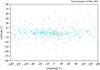 |
Fig. 4. Galactic distribution of objects in the GAPN-EDR3 sample. |
Figure 5 shows the distance distribution for the GAPN-EDR3 sample. In comparison with the general sample distribution, we see that the distances tend to be closer, there being only a few PNe farther than 7 kpc; around 50% of them are located closer than 2 kpc; and, from a distance of approximately 1.5 kpc onward, we found that the number of objects started to decrease progressively. The mean distance of this distribution is 2.45 ± 0.96 kpc. In Table A.2, we provide the parallaxes and distances (with their uncertainties) of all objects in the GAPN-EDR3 sample, together with the radial velocities (Velrad) for some of them. The full table is available at CDS.
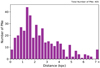 |
Fig. 5. Distance distribution of the GAPN-EDR3 sample. |
It is interesting to compare the new Gaia EDR3 distances to PNe with those obtained by other authors using different methods. These comparisons are displayed in different graphs. In each one, the blue line indicates the 1:1 relation between both distance derivations, while the red line represents the linear regression between them. Individual data points are drawn with error bars for each distance derivation.
We first compared EDR3 distances with those obtained in Paper I from Gaia DR2. In Fig. 6, we see that despite there being a significant dispersion for some objects, the two distance distributions are mostly equal, the only difference being that the EDR3 distances are more accurate than those of DR2, especially for distances above 2 kpc. We note, however, that for some stars that have been assigned significantly greater distances in EDR3 than in DR2, the errors in EDR3 may be greater than those of DR2.
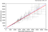 |
Fig. 6. Distance comparison between Gaia DR2 and Gaia EDR3. The blue line indicates the 1:1 relation, while the red line represents the linear regression between them. These lines are also shown in the figures that follow. |
If we compare EDR3 distances with others also obtained with astrometric methods, such as those provided by Harris et al. (2007), we see that there is also reasonable agreement between both distance determinations, as in the case for DR2 distances. Figure 7 displays this comparison, which only depicts distances below 800 pc.
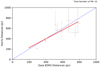 |
Fig. 7. Distance comparison between Harris et al. (2007) and Gaia EDR3. |
Other methods of estimating distances are based on statistical procedures, such as that used by Stanghellini & Haywood (2010). If we compare these distances with those reported here (Fig. 8), we see that in general they are overestimated, which had already been found with the comparison with distances in DR2 (Paper I). This time, we find a positive bias of around 400−500 pc, a lower value than found before.
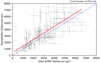 |
Fig. 8. Distance comparison between Stanghellini & Haywood (2010) and Gaia EDR3. |
Non-LTE model stellar atmosphere fitting was also used to derive distances to CSPNe. This method consists of obtaining the stellar effective temperature and surface gravity from spectra and uses evolutionary tracks for post-AGB stars to estimate masses and distances. The method was proposed for the first time by Mendez et al. (1988) to estimate a few PNe distances and was later used by Napiwotzki (2001) to estimate distances for a large sample of PNe. If we compare these distances with those of EDR3 (Fig. 9), we see that, as in our DR2-based study, Napiwotzki’s distances are overestimated in comparison with ours. As we did in our previous study, we divided the CSs into high and low temperature sets (see legend). We observed that those with lower temperatures conform more closely in terms of their EDR3 distances with those of Napiwotzki. In contrast, high temperature CSs showed a bias between two distance determinations that go from 250 pc (for the closest ones) to more than 500 pc (for the farthest ones). It is possible that this effect occurs because non-LTE models do not take into consideration line-blanketing for metals.
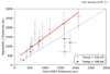 |
Fig. 9. Distance comparison between Napiwotzki (2001) and Gaia EDR3. Sources are divided in two groups according to their effective temperatures. |
We now compare EDR3 distances with those derived by Frew (2008), who used a distance scale to CSPNe based on a statistically derived relation of Hα surface brightness evolution with nebular radius. As can be seen in Fig. 10, there is no clear relation between these distance derivations. We can only say that for the closest PNe (below 1200 pc) Frew’s distances tend to be overestimated in comparison with ours, whereas they tend to be underestimated for greater distances (over 1200 pc).
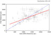 |
Fig. 10. Distance comparison between Frew (2008) and Gaia EDR3. |
Finally, Schönberner et al. (2018) calculated the distances to 15 round-shaped PNe by measuring the expansion velocity of the nebular rim and shell edges, and correcting the velocities of the respective shock fronts with 1D radiation hydrodynamic simulations of nebular evolution. In Fig. 11, we see a comparison between these distance derivations and those from EDR3. The result is very similar to the one reported in Paper I, and we find no bias or clear relation between these distance derivations. The nearest nebulae (below 1800 pc) have overestimated distances in the work of Schonberner when compared with EDR3, whereas for distances greater than 1800 pc they seem to be underestimated. Nevertheless, the number of objects is fairly small and the errors quite large, so no firm conclusions may be drawn.
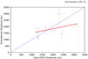 |
Fig. 11. Distance comparison between Schönberner et al. (2018) and Gaia EDR3. |
3.2. Nebular sizes and morphology
Knowledge of the distances to PNe, together with the measured angular sizes of the nebulae, allows us to estimate their physical radii. We obtained the angular sizes from the HASH database, where minor and major nebular diameters are provided for almost all (99%) of the PNe in our sample. Using mean angular radii as a proxy for true angular radii, we then obtained the physical radii.
Figure 12 shows the nebular radius distribution for our objects in the GAPN-EDR3 sample. Fifty-four per cent have a radius shorter than 0.3 pc (1 light-year approximately). However, there are PNe with much greater radii, which illustrates the diversity of evolutionary states in the sample. In fact, around 14% of the PNe have a radius greater than 1 pc. These must be evolved nebulae, with their CSs already being at the white dwarf stage. The mean radius of the entire sample is 0.59 pc. For more information, both angular and physical radii are listed in Table A.2.
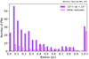 |
Fig. 12. Radius distribution of the GAPN-EDR3 sample. |
For a more detailed analysis, we divided the PNe into two sets: those located close to the Galactic plane (latitudes in the interval ±15°) and those located far from the Galactic plane (other latitudes). As shown in Fig. 12, the PNe of the first group tend to be smaller than those of the second group, which are more evenly distributed over a wide range of sizes. Thus, we may conclude that PNe in the Galactic plane tend to be younger than the others since they are still smaller in size.
As is well known from the pioneering work of Greig (1972), PNe display a wide variety of morphologies. The most common ones are round, elliptical, and bipolar, but there are also others with star-like (or point-like), asymmetrical or irregular shapes. Logically, the morphological classification of PNe is subject to the uncertainty because of projection effects, and also because of the resolution and sensitivity of the images. If we analyse the morphologies in the GAPN-EDR3 sample (endorsing the HASH morphological cataloguing), we find that 40.2% of the PNe are elliptical, 22% bipolar, 18.8% round, 2.7% star-like, 2% irregular, and 1.2% asymmetrical. We note that we have a significant percentage of PNe (13.1%) of a non-classified morphology. In order to check if these percentages might be biased owing to a brightness effect (bipolars tend to be brighter on average), we calculated the morphological distribution for nebulae at distances of less than 2 kpc, which can be set as our approximate limit of completeness. As a result, we obtained a similar morphological distribution (37.2% elliptical, 24% bipolar, and 16.8% round).
It is interesting to investigate whether any relation exists between PNe morphological types and their location in the Galaxy. Previous studies (see, for instance, Peimbert & Torres-Peimbert 1983; Zuckerman & Gatley 1988; Corradi & Schwarz 1995; Manchado 2004) have shown that bipolar nebulae tend to be high-excitation, type I nebulae, and that they are located closer to the Galactic plane than elliptical ones. This led to the conclusion that bipolars have probably evolved from a more massive disc population, although this conclusion was based on a poorly populated sample of objects.
Our data and accurate distances allow us to study this relationship in detail. From latitudes and distances, we calculated the Galactic height (z) of the PNe in our sample. We then plotted (Fig. 13) the PNe from the main morphological categories (elliptical, bipolar, and round) as a function of their Galactic longitude and height. A glance at this figure seems to indicate that there really is a lack of bipolar nebulae at high Galactic heights. To check this, we divided the PNe into two sub-samples according to their morphology (bipolar and non-bipolar). For each set, we displayed the distribution of the nebula population as a function of Galactic height (see Fig. 14). Then, by fitting a logarithmic curve to these distributions, scale height values (Hz) were calculated for both populations:
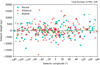 |
Fig. 13. Galactic distribution of round, elliptical, and bipolar PNe. |
As can be seen, we obtained considerably different scale height values (with small uncertainties) for each morphological group. Bipolars are more concentrated in the Galactic disc region, so our data lend support to the conclusion that, in general, they come from a different population. Figure 14 shows Galactic height distributions for each morphological group, together with their derived population curve. The scale height value for each set is shown by a vertical dotted line. The particular Galactic height values are listed in Table A.2.
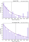 |
Fig. 14. Galactic height distributions for bipolar (up) and non-bipolar (down) PNe. The dark curve represents the PNe population as a function of Galactic height per 50 pc bin, and the dotted vertical line indicates the scale height. |
We also studied the relationship between morphological type and nebular size. If we calculate the mean radius (⟨R⟩) for bipolar and non-bipolar PNe, we obtain the following values:


As a result, we obtained that bipolar PNe tend to be considerably smaller than the others, with a mean radius of less than a half that of the non-bipolar mean radius, although the uncertainty values are considerably higher in this case. In the following section, we study the evolutionary properties (such as temperature, mass, and age) of CSPNe and analyse possible relationships between nebular morphology and these other properties.
3.3. Expansion velocities and kinematic ages
Another interesting property to study is the kinematic age of PNe. This parameter measures the time elapsed since the envelope was ejected from the CS crust, assuming that a constant representative expansion velocity for the nebula applies for its entire life span. In Paper I, we discussed the problems with measuring expansion velocities and interpreting them in terms of the hydrodynamical evolution of real objects. For our new sample, we explored the literature for expansion velocity measurements and took most of the values from the Frew (2008) compilation of expansion velocities for a large set of PNe. Kinematic ages from Weinberger (1989) were also included. From these expansion velocity values and physical nebular radii, we were then able to derive kinematic ages under certain assumptions and constraints that needed to be considered.
We first of all worked on the supposition that the expansion velocity is constant throughout the nebular phase and that this velocity was the same in all directions of the nebula. Hence, we only considered the case of approximately round-shaped nebulae. We proceeded to select a sample of PNe with minor semi-axis size values with at least 75% of the size of the major semi-axis: Rmin ≥ 0.75 ⋅ Rmax. In compliance with Jacob et al. (2013), we also rejected those PNe considered as H-deficient or containing close binaries because their evolution follows a different path. We thus selected a sample of 65 PNe with known expansion velocities that fulfilled these conditions.
Hydrodynamical modelling of the evolution of PNe by Jacob et al. (2013) indicates that expansion velocities will probably not be equal for all their layers, and that it is advisable to apply a correction factor to the measured velocities in order to obtain more realistic mean expansion velocity values. Following the prescriptions in Jacob et al. (2013), we decided to use an overall value of 1.5 as the correction factor, just as we did in Paper I.
The obtained expansion velocity distribution is shown in Fig. 15. Most (78%) of the selected PNe have expansion velocities between 10 and 50 km s−1, while the fastest nebula expands with a velocity of almost 80 km s−1. The mean expansion velocity of this sample is 32 ± 13 km s−1, slightly lower than the one obtained in Paper I (38 ± 16 km s−1), but within the uncertainty interval. Particular expansion velocity values for each of the 65 (uncorrected) PNe are listed in Table A.3.
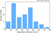 |
Fig. 15. Expansion velocities distribution of 65 selected objects from the GAPN-EDR3 sample. |
From the expansion velocities, we were able to calculate the corresponding kinematic ages using the following simple relation:

The resultant kinematic age distribution is shown in Fig. 16. As can be seen there, the majority (66%) of the PNe are quite young, with a kinematic age below 10 kyr. However, there is a considerable fraction (18%) of older PNe, with ages above 20 kyr. The reason why our results could be biased towards younger ages is probably that young PNe are easier to detect than old ones, as they are generally brighter. The mean kinematic age of our sample is 17.8 ± 3.0 kyr. Table A.3 lists the kinematic age values of the PNe in this sample.
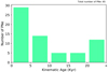 |
Fig. 16. Kinematic age distribution of 65 objects selected from the GAPN-EDR3 sample. |
We were also able to estimate the maximum age of a PN or, equivalently, the maximum time that a PN is visible before becoming completely diluted in the interstellar medium. This concept is known as visibility time (Tvis). For this calculation, we need to consider a maximum mean nebular radius for the PNe (reaching, according to Jacob et al. 2013, 0.9 pc, which is in good agreement with what we state in Sect. 3.2). By dividing this value by the obtained mean expansion velocity, we then calculated the following visibility time:
In conclusion, a PN is expected to have a mean lifetime of approximately 28 kyr. This value is higher than that obtained in Paper I (23.4 ± 6.8 kyr), but both values are in agreement to within their uncertainties.
4. Evolutionary state of CSPNe
Knowledge of accurate distances for the CSs in the GAPN-EDR3 sample can be combined with brightness and effective temperature values from the literature to locate them on an HR diagram. Making use of evolutionary tracks for post-AGB stars, their evolutionary state can then be estimated (i.e. their masses and ages).
4.1. Temperatures and luminosities
Literature about CSPNe effective temperatures mostly contains measurements obtained by the Zanstra method (Zanstra 1928), which is based on measuring HI or HeII nebular fluxes. So, similarly to what we did in Paper I, we used literature effective temperature values obtained by this method. In this way, we were able to collect consistent temperature values for a total of 151 stars in our sample from Frew (2008), Frew et al. (2016), Gleizes et al. (1989), and Guerrero & De Marco (2013).
To calculate stellar luminosities, we evaluated the bolometric magnitudes from brightness measurements in Gaia or other photometric bands. CSPNe are hot stars, with effective temperatures well beyond the limit of 8000 K that Gaia DPAC set for bolometric corrections and luminosities derived from DR2 observations (Andrae et al. 2018). As in Paper I, we decided instead to use the Vacca et al. (1996) relationship for bolometric corrections in the visible band, so we needed to compile V magnitudes for our sample of CSPNe. GAPN-EDR3 V magnitudes were generally obtained from the studies of Frew (Frew 2008; Frew et al. 2016), complemented with data from the APASS database3, Tylenda et al. (1991), and Weidmann et al. (2020). We were thus able to obtain V magnitudes from the literature for a total of 326 stars in GAPN-EDR3 (80% of them).
Given the possibility that some of our CS identification did not match those in the literature, we decided to compare the de-reddened G and V magnitudes for each star. Gaia EDR3 online documentation4 provides a relationship used to estimate the Johnson V magnitude from the GaiaG, GBP and GRP magnitudes (henceforth, VG). Such a relationship was calculated by Gaia DPAC using data with a lowest colour limit value of (GBP − GRP) = − 0.5, but we now show that it also works well with blue stars beyond that limit. In fact, if we calculate the difference between literature V values (VL) and G-derived V values (VG), we obtain a mean value and standard deviation of |VG − VL| = 0.227 ± 0.054 mag for the sample of stars with bluer colours (GBP − GRP ≤ −0.5), and |VG − VL| = 0.278 ± 0.098 mag for the remaining objects in the sample. The comparison between the VG and VL magnitudes is shown in Fig. 17. In order to filter out those CSPNe with suspect V magnitudes from the literature, we use the term ‘mild outlier’ as a threshold for such uncertain data. To estimate this threshold value, we obtained the differences |VG − VL| and calculated their distribution interquartile range; namely, the difference between the third and first quartiles: (Q3 − Q1). As is well known, the mild outlier limit is set as 1.5 times the interquartile range. Following this procedure, we obtained a threshold value of 0.382 mag (see Fig. 17). We then decided to discard those CSPNe with |VG − VL| greater than this value, and we finally obtained 253 CSPNe with reliable VL magnitude values. These V magnitudes (and also the G magnitudes) are listed in Table A.4.
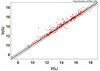 |
Fig. 17. Comparison between V magnitudes from the literature (VL) and V magnitudes calculated from Gaia passbands (VG) for 326 objects of the GAPN-EDR3 sample. The black central line indicates the 1:1 relation, while grey lines indicate the threshold for the mild outliers. |
We also had to consider the interstellar extinction for each star. As explained in Sect. 2, we obtained these values from Bayestar and SFD dust maps. The Galactic position of each source was employed to estimate the interstellar extinction. However, we know that the nebula itself might also contribute to the extinction of the CS, especially in young and compact nebulae. So, to be more thorough, we looked for specific literature extinction information for the selected stars. For consistency, we decided to obtain these values from the studies of Frew (Frew 2008; Frew et al. 2016), complemented by extinction values from Tylenda et al. (1992) and Cahn et al. (1992). For the remaining CSPNe (51% of them), we used the general extinction obtained from the dust maps. All these extinction values are shown in Table A.4.
With this procedure, we were able to calculate the absolute visible magnitude (MV) for the 253 CSPNe (with reliable VL magnitudes) cited previously using the following relation:

where V is the visible magnitude, D the distance, and AV the interstellar extinction.
The absolute bolometric magnitude (MBol) could then be calculated from the absolute visible magnitude (MV) and the effective temperature (Teff) via the relation of Vacca et al. (1996):

Finally, we obtained the stellar luminosity as:
where MBol⊙ = 4.75 is the Sun’s absolute bolometric magnitude.
As we compiled effective temperatures for a limited set of objects in GAPN-EDR3 sample, we were able to estimate the luminosities for a total of 121 CSPNe. In order to analyse the evolutionary state of such stars using standard H-rich evolutionary tracks, we then had to exclude those objects catalogued as H-deficient stars, as well as known close binary stars. For the identification of these types of objects, we followed the classification of Boffin & Jones (2019), Weidmann et al. (2020), and Jacob et al. (2013). We finally ended up with a sample 74 CSPNe, whose evolutionary state could be studied from their temperature and luminosity values. All these values are presented in Table A.4. This sample of CSPNe has a very high reliability rate, as 85% of them belong to identification reliability group A, and only 15% belong to group B.
4.2. Mass and evolutionary age
As in our previous DR2 study, the next step was to plot our selection of 74 CSPNe with reliable temperature and luminosity determinations on an HR diagram and compare their location with the predictions of evolutionary models for the post-AGB phase. As in Paper I, we decided to use the post-AGB evolutionary tracks of Miller Bertolami (2016) because of the updated opacities, nuclear reaction rates, and consistent treatment of stellar winds for the C- and O-rich regimes in that paper. Miller Bertolami computed the evolutionary sequences from the ZAMS to the post-AGB phase for stars in the initial 0.8–4 M⊙ mass range, which corresponds to post-AGB masses from 0.5 to 0.85 M⊙, which is the most relevant range for CSPNe. In the case of solar metallicity (which we assumed), the upper mass limit for main sequence stars is 3 M⊙.
In these models, a temperature limit of 7000 K (log(Teff) = 3.85) is set as the reference for the beginning of the fast part of the post-AGB evolutionary process, when winds play only a secondary role in setting the timescales. The CSPNe evolutionary age is calculated by adding a transition time that begins earlier, when the envelope mass reaches 1% of the stellar mass and the AGB stage ends (see Miller Bertolami 2016 for details). Following the evolutionary paths, the stars warm up to an approximately constant luminosity. After reaching the maximum temperature, they start to cool down and lose luminosity until they eventually reach a stable phase as white dwarf stars. As we have seen (depending on the mass), the whole PN phase time span can last tens of thousands of years.
In Fig. 18, the location of our CSPNe is set in the HR diagram, together with the evolutionary tracks. As can be appreciated, all the points in this diagram are plotted together with their corresponding error bars. We assumed relative errors of 10% in temperature. Taking into account the uncertainty in luminosity, we calculated them by error propagation from the uncertainties in distance (low and high), V magnitude, and temperature. Then, by interpolation between the tracks, we were able to estimate the progenitor mass and evolutionary age for all the CSPNe.
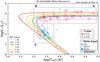 |
Fig. 18. Location in the HR Diagram of the 74 CSPNe with known luminosities and temperatures in the GAPN-EDR3 sample, together with evolutionary tracks by Miller Bertolami (2016). Information about their spectral classification is also provided. |
Figure 19 shows the mass distribution for the 74 CSPNe selected. Around 70% of the CSPNe in our sample come from progenitor stars with masses below 2 M⊙, and we obtain a mean value for the progenitor mass of 1.8 ± 0.5 M⊙. Only a few stars (12% of the sample) lie slightly beyond the 3 M⊙ track. Particular mass values are listed in Table A.4.
Concerning the evolutionary age (see Fig. 20), although we found a large variety of values, most of the CSPNe are quite young, as around 50% have ages below 10 kyr. Within this group, the age distribution is quite constant, as can be seen in the inset of the figure. On the other hand, we detected several objects with ages far above 60 kyr. These ages correspond to CSPNe located towards the end of the evolutionary tracks (see Fig. 18). These stars have lost almost all of their nebulae and have already reached the white dwarf phase. The remaining CSPNe present intermediate evolutionary ages between 10 and 60 kyr. We note that, following the prescriptions of Miller Bertolami (2016), we added a certain quantity corresponding to the transition time to the ages obtained from the tracks. As we already mentioned, this time extends from the beginning of the post-AGB phase to the instant at which the CS reaches the temperature of 7000 K set by this model. This time interval lasts between approximately 1 and 36 kyr, depending on the progenitor masses. All the evolutionary ages are listed in Table A.4.
In general, the location of the CSPNe in the HR diagram adequately fits the region covered by the models, with only one clear outsider: the CS of the HaWe 13 nebula. This is an hgO(H) white dwarf with a temperature of 68 000 K and luminosity log(L/L⊙) = 2.43. Being a white dwarf star, it should have yet a higher temperature for that luminosity or should otherwise already have a lower luminosity for that temperature.
4.3. Spectral types
We retrieved the spectral classifications for those stars located in the HR diagram from Weidmann et al. (2020). In Fig. 18, we plot those objects that are classified as O-type stars with a red symbol, white dwarf stars with a blue symbol, and those of unknown classification with a grey symbol. Weidmann et al. (2020) reviewed the evolutionary paths followed by stars until the PN stage from an observational point of view. Although there is no generally accepted theoretical model, it is agreed that two groups of H-rich and H-poor stars, single stars seeming to follow two evolutionary post-AGB channels, according to their H-rich and H-poor composition (Löbling et al. 2019). Weidmann et al. (2020) discuss the spectral types associated with different masses and the uncertainties concerning interpretation of spectral sequences. For their representation on an HR diagram, we discarded objects with spectral types associated with H-deficient stars, as well as all objects susceptible to binarity. Figure 18 shows spectral types divided into early O-type (0–4) stars, late O-type (5–9) stars, O-type hot subdwarfs (sdO), intermediate evolved objects (hgO(H)), and H-rich white dwarfs (DA(O)).
A fairly coherent sequence of spectral types in our HR diagram became notably apparent: O-type stars were located in the constant luminosity region of the tracks, with late O-type stars generally being located in the right part of this region (cooler temperatures) and early O-type stars tending to be located at a later stage (hotter temperatures): a scenario that supports a good correspondence between an object’s position in the diagram and its spectral classification. Stars classified as white dwarfs were also located in the region where they were expected to be, near the elbow that marks maximum temperatures and in the region where the central star begins to cool down and drastically decrease in luminosity. O-type hot subdwarfs tended to be located in the most luminous zone. We then found hgO(H) intermediate objects and in the most evolved region there were H-rich white dwarfs. Only a few objects appeared not to conform to these rules. The particular spectral types of GAPN-EDR3 objects are listed in Table A.2, particularly for those objects located in the HR Diagram, in Table A.4.
4.4. HR diagram analysis per region
For a more detailed study, we separated the HR diagram into three regions (see Fig. 18) according to the evolutionary status of the objects. As in Paper I, we defined the regions as follows: region A corresponds to an early PN phase, with stars increasing their temperatures (till log(Teff) = 4.8) at a fairly constant luminosity ( ); region B corresponds to the same flat luminosity part, but for higher temperatures (until the maximum temperature); and region C corresponds to the late-PN phase with lower luminosities than the previous regions and decreasing temperatures. Almost all objects located in region A are O-type stars. On the other hand, almost all those located in region C are white dwarf stars. While in region B, we find several objects of both types, the majority of them being O-type stars.
Table 1 shows the mean values and standard deviations of the evolutionary parameters in each region (nebular radius, CSPNe temperature and age, and progenitor star mass). Regarding the nebular radius mean value (⟨R⟩), the clear and expected increase in size from region A to C is significant, going from less than 0.1 pc to almost 1 pc. So, the properties of stars and the derived size of their nebulae are in agreement with what is expected for these rapidly evolving objects. On the other hand, we can observe that the progenitor star mass mean value (⟨M⟩) remains approximately constant throughout the three regions, with a mass around almost 2 M⊙. This is what we expected, as this parameter does not depend on the evolutionary phase reached by the PN. Evolutionary age mean values (⟨Tevo⟩) tend to increase considerably from region A to C, although there is great dispersion, as their standard deviations are considerably high, especially in region C. That is probably due to the presence of very old objects that have almost entirely lost their nebulae and have already become a white dwarf. Finally, we have also included the corresponding mean values for the kinematic ages (⟨Tkin⟩) obtained in the previous section in this table. As expected, these also show a similar tendency to increase as evolutionary ages. We note that there are four CSPNe located outside the three regions; these are generally stars that are too evolved to be considered for this evolutionary analysis.
Mean values (with uncertainties) of different parameters in three regions of the HR diagram.
As we said previously, in Paper I we performed a similar analysis using Gaia DR2 parameters, and now we have been able to locate more CSPNe on the HR diagram with better quality parameters, so these results should be more consistent. Furthermore, some discrepant objects located away from the evolutionary tracks in the previous study are no longer present. These objects were discarded for several reasons: misclassification as PNe according to the HASH database, a new source in Gaia EDR3 identified as CSPNe, or their being catalogued as a close binary or H-deficient star in Weidmann et al. (2020). In summary, in Paper I we had slightly higher values for nebular radii and lower values for the evolutionary age, but the mean values generally follow a similar trend and are compatible to within their uncertainties.
Returning to the morphological study, we can now analyse the evolutionary state of each of the main morphological groups (elliptical, bipolar, and round) by obtaining the mean value of their different evolutionary parameters, as shown in Table 2. We note that 96% of the CSPNe in this sample are catalogued within these main morphological types. According to the results, we are able to confirm that bipolar PNe are notably smaller than the other types (as we postulated in Sect. 3.2), with a mean radius of only 0.2 pc. Consequently, our sample of bipolar PNe tend to be younger than elliptical or round ones. Regarding the CSPNe temperature and progenitor mass, the three morphological types show similar mean values, and no definitive conclusions may be drawn concerning a possible relationship between these properties and nebula morphological type. It should be taken into account that a round nebulae count may be influenced by projection effects (7% of ellipticals can be seen as round, Manchado 2004).
Mean values (with uncertainties) of different parameters from the main three morphological types.
5. Binary CSPNe
It is well known that the large variety of PNe shapes has been related to binary companion interaction (Jones & Boffin 2017). Gaia astrometry may provide some clues to assess the importance of binarity and stellar multiplicity in the formation and evolution of CSPNe. Some authors have proposed that even distant binary companions may provide an alternative mechanism for the formation of highly aspherical morphologies by influencing the direction of collimated winds from the parent star (Garcia-Segura 1997, see discussion in Sahai & Trauger 1998). Therefore, we found that it may be useful to search for binaries by using Gaia EDR3 precise astrometry.
In Paper II, we performed a search for comoving objects in the fields of PNe with good determinations of parallaxes and proper motions. Several cases were found and we were able to estimate mass values for both the CSs and their binary companions compatible with a joint evolutionary scenario. It should be noted here that none of the systems found in such work was close enough to generate the necessary gravitational torque that could result in an impact on the morphology of the nebula, according to the models by Garcia-Segura (1997). More precise astrometry in the EDR3 archive allowed us to update the aforementioned search of comoving companions in our GAPN-EDR3 sample.
The Gaia object detection pipeline and the astrometric solution for multi-epoch observations in the EDR3 catalogue provides users with parameters that can be used to search for evidence of close binary pairs. We performed a statistical test to look for such evidence of binarity among our sample targets with ‘red’ and ‘blue’ (GBP − GRP ≤ −0.2) CSs.
5.1. Search for wide binaries in GAPN-EDR3
In Paper II, we showed that high-precision Gaia parallaxes and proper motions allow us to find wide binary companions as comoving objects. In a similar way, we used the improved Gaia EDR3 astrometry to search for such types of resolved binaries in our GAPN-EDR3 sample. We define sources that have celestial coordinates and astrometric parameters (parallaxes (w) and proper motions in RA (PMRA) and Dec (PMDec) coordinates) compatible with a gravitational bond to within the observational errors as comoving objects. We note that as radial velocities are, in general, unavailable for the companion stars, we limited our study to movements on the plane of the sky.
The procedure pursued is equivalent to that in our previous work. We first selected all the Gaia EDR3 sources within a radius of 120 arcsec around each of our CSPNe. We then discarded those objects without parallax and obtained 630 objects on average in each PNe neighbourhood. The parallaxes (and uncertainties) for these objects were corrected as explained at the beginning of Sect. 4. In this case, we also needed to correct the proper motions and their uncertainties, and this was done following the relations in Lindegren et al. (2018). Then, only objects with accurate astrometry were selected, that is, those with relative errors below 30% in parallax, distance and proper motions. On average, we ended up with around 50 binary companion candidates per PN. We note that the central stars in the GAPN-EDR3 sample also had to pass such filtering in proper motions, which is why we lost a few of them and finished with 357 CSPNe.
The next step was to implement an algorithm to detect the comoving objects to any CSPNe. As in Paper II, we adapted the procedure used by Jiménez-Esteban et al. (2019). The method consists of selecting objects for which the three astrometric parameters (w, PMRA, PMDec) differ less than 2.5 times σ in comparison with those of their corresponding CSs, where σ is the highest uncertainty value between the candidate object and the CS for each parameter. After executing the algorithm, we were able to detect 85 possible binary (or multiple) systems as CSs in the GAPN-EDR3 sample.
However, many of those binary companions might be too far from the CSPNe to be truly gravitationally bound, and they might only share the same astrometric parameters by chance. In Paper II, we included a discussion of the expectation for the maximum projected physical separation between binaries. Following Zavada & Píška (2020), we set this maximum value at 20 000 AU. By using the same constraint here, we finally isolated eight wide binary or multiple systems.
In comparison with the binary CSPNe found in Paper II, we confirm the presence of five wide binary systems (Abell 24, Abell 33, Abell 34, NGC 3699, and NGC 6853). For more details, we invite the reader to consult Sect. 3 of Paper II. On the other hand, we could not, for different reasons, include in the present study three possible wide binary systems found in Paper II: NGC 246 (because its CS did not fulfil the astrometric quality constraints to be included in GAPN-EDR3), SB 36 (because it is not catalogued as a PN in the HASH database), and PHR J1129–6012 (because the identification of the CS was not clear). Apart from the five systems mentioned, we detected three possible new wide binary systems for PN G030.8+03.4a, NGC 6720, and NGC 6781. In Table 3, we show the astrometric parameters (coordinates, separation, distance, parallax, and proper motions) and Gaia colours of both components belonging to the systems cited before.
Data from new binary systems detected in GAPN-EDR3.
The first new binary system detected corresponds to the planetary nebula NGC 6720 (Fig. 21), also known as the Ring Nebula. This nebula is located at a distance of almost 800 pc from the Sun and has an elliptical shape, with a mean radius of around 30 000 AU (0.147 pc). We detected a binary companion with a projected separation of more than 14 000 AU from the CS. According to its absolute G magnitude (MG = 8.16 mag) and its colour (GBP − GRP = −0.23), it must also be a white dwarf.
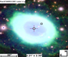 |
Fig. 21. Image of a possible binary system in NGC 6720, showing the location of both the CSPN (with a cross) and the comoving companion. Image from the Aladin sky atlas (CDS). |
We detected another binary system in the bipolar planetary nebula NGC 6781 (Fig. 22), which is located almost 500 pc from the Sun. It has a similar size to that of the Ring Nebula, with a mean radius of around 31 000 AU (0.15 pc). In this case, we detected a binary companion with a projected separation of less than 5000 AU from the CS. Using the Virtual Observatory SED Analyser (VOSA) tool from the Spanish Virtual Observatory (SVO) platform5, we were able to obtain some evolutionary parameters of the companion star. From its coordinates, distance and extinction, we first retrieved its photometry and built its spectral energy distribution (SED). By fitting this SED to NextGen models (Allard et al. 2012), we were then able to calculate its effective temperature (Teff = 3400 K) and luminosity (log[L/L⊙]= − 1.18). These values correspond to an M-type star. Finally, by plotting the star in an HR diagram and using NextGen evolutionary tracks, we estimated a mass of 0.35 M⊙ for the companion star. The CS with 0.60 M⊙ is considerably more massive than the companion star, as its mass in the MS would be about 2.21 M⊙ according to the Miller Bertolami models. The presence of a binary system in this nebula was proposed a few years ago by Douchin et al. (2015), who catalogued it as an M3-type star, in good agreement with the values found here.
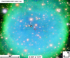 |
Fig. 22. Image of a possible binary system in NGC 6781, showing the location of both the CSPN (with a cross) and the comoving companion. Image from the Aladin sky atlas (CDS). |
The third binary system detected by our algorithm is located in the nebula PNG 030.8+03.4a (Fig. 23). This PN has a star-like morphology and is also close to the Sun, at a distance of around 550 pc. Here, we detected a binary companion with a projected separation of slightly over 5000 AU from the CS. In this case, by fitting its SED through the VOSA tool, we estimated its temperature at 3500 K with a luminosity of log[L/L⊙]= − 0.94, which corresponds to an M-type star. In addition, by using the models evolutionary tracks, we obtained a mass of 0.32 M⊙ for this companion star.
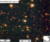 |
Fig. 23. Image of a comoving system in PNG 030.8+03.4a, showing the location of both the CSPN (with a cross) and the companion. Image from the Aladin sky atlas (CDS). |
During the analysis of our wide binary systems candidates, a group of stars that did not strictly meet our astrometric criteria attracted our attention in the nebula Fr 2–42 (Fig. 24). As this PN is located a fairly short distance from the Sun (around 130 pc), if any companion object orbited the centre of mass of the system, the orbital movement might explain, to a certain degree, certain differences in the observed proper motions between the system components. In particular, we found two possible companions to the proposed CSPN. Their coordinates, Gaia colours, and other astrometric properties are listed in Table 3. All three stars in the system have colours and brightnesses corresponding to hot white dwarf stars, thus rendering this possible triple system interesting for further study. Despite the stability of this type of system in the nebular phase being rather dubious (Jones et al. 2019), the existence of at least one of them (NGC 246) has been proven.
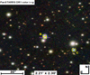 |
Fig. 24. Image of a possible triple system in Fr 2–42, showing the location of the CSPN (with a cross) and the two comoving companions. Image from the Aladin sky atlas (CDS). |
5.2. Discussion concerning close binaries
Even though binary stars with separations of less than 0.18−0.60 arcsec are not included as separated sources in Gaia EDR3 (Lindegren et al. 2021), the excellent quality of Gaia’s source detection algorithm, the crossmatch procedure, and the joint astrometric solution for parallaxes and proper motions allow us to address the detection of close binarity signs in our set of CSs by analysing the statistics of these measurements.
We were able to relate cases with statistically noisy measurements with the presence of a close binary companion that might be interfering with the CS detection and its astrometry. In particular, we analysed the following parameters that are available in the EDR3 archive: astrometric excess noise (measures the disagreement between the observations of a source and the best-fitting standard astrometric model), image parameter determination procedure (IPD) harmonic amplitude (measures the deviation in the image centroid fitting), RUWE, and coordinate uncertainties in RA and Dec.
Apart from anomalies in the values of parameters related to image detection or astrometry quality, the presence of a close companion star could explain the red colour of some of the CSs detected. So it could be hypothesised that red CS quality parameters would be statistically different from those measured for blue CSs. Consequently, for this study, we decided to recover some objects from reliability group C that were discarded mainly because of their deep red colour (see Fig. 2), and that might be useful for this analysis. In particular, we included those group C objects located within 50% of their nebular radius, as this is the maximum permitted distance for objects in groups A and B. We then applied to this extended sample the same filtering constraints that were applied to select the GAPN-EDR3 sample (see Sect. 3), so we finally obtained a set of 464 stars (405 from GAPN-EDR3 and 59 from group C). These 59 extra objects are available at CDS as an extension of Table A.1.
We then divided this sample into blue (GBP − GRP ≤ −0.2) and red stars (GBP − GRP > −0.2) and calculated the mean values of the above-mentioned parameters in each subset. As a result, we found that stars in the red CS sample had slightly higher mean values for these parameters, as is shown in Table 4. This means that their image centroid fit gives a statistically more smeared solution, that the disagreement between the observations of a source and the best-fitting standard astrometric model is higher, and that the RUWE values, RA, and Dec coordinates are all noisier. This might be because red stars, compared to blue ones, tend to have parameters more related to the presence of unresolved binary systems.
Mean values (with uncertainties) of the astrometric and image-fitting quality parameters for blue and red CSPNe samples.
In order to test this hypothesis quantitatively and give a measure in statistical terms of the difference between both samples of CSs, we decided to carry out a statistical test to measure the significance of the similarity or dissimilarity of both samples with reference to the aforementioned parameters. We used the Kolmogorov–Smirnov6 statistical test. This is a non-parametric test that quantifies the distance between the empirical cumulative distribution functions of two samples. The null distribution of this statistic is calculated under the null-hypothesis that the samples are drawn from the same distribution. From this analysis, two statistical parameters are obtained that provide information on the similarity between both samples: the p value and the D value. If the p value is below a certain α value (usually 0.01 or 0.05), the two samples are said to be different; otherwise, there could be some similarities. We considered α = 0.01 for a highest level of significance, corresponding to a 99% confidence in the results. On the other hand, if the D value is greater than a certain value (Dα), we can say that the two samples are different; otherwise, the samples could be similar. This Dα, which depends on the sample populations and on α itself, in this case takes a value of 0.153. After running this test, we obtained for each parameter the p and D values shown in Table 4.
In conclusion, our results exclude the possibility that the samples are drawn from the same population and therefore point to very low coincidences between the parameters of our blue and red CSPNe. Only for the RUWE parameter did we obtain any evidence of a possible similarity between both samples, as shown in Table 4. However, it may be pertinent to recall that objects in the analysed samples were previously filtered in terms of the quality of the RUWE parameter, which probably influenced the relevance of this parameter in the test. For the other parameters we obtain results that reject any similarity. This led us to the conclusion that red CSPNe properties are drawn from a very different population from that of the blue CSPNe, which could be interpreted as evidence of a greater incidence of close binarity among red CSPNe.
We find it useful to discuss the results by Chornay et al. (2021), in which Gaia DR2 was used to identify close binary central star candidates based on the released multi-epoch photometry and the excess photometric uncertainty. A Kolmogorov–Smirnov test between our red sample and a sample from Chornay et al. (2021) of close binary candidates (EDR3 data) results in four out of five of the astrometric parameters coming from a similar distribution, while a comparison between our blue sample and that from those authors results in similarity for only two out of five astrometric parameters. These results reinforce our conclusion about the possible binary nature of red CSPNe.
6. Conclusions
Using the recently published Gaia EDR3 catalogue, we identified, with different degrees of reliability, the CS for a total of 2035 Galactic PNe. To achieve this, we developed an algorithm that, considering both the colour of the star and its distance to the nebular centre, selects the source with the best parameters for the CS to be located within a radius of 20 arcsec around each planetary nebula. For those PNe with known parallaxes in EDR3 (1725 PNe), we obtained their distances from the Bayesian statistical method of Bailer-Jones et al. (2021).
A set of 405 CSs, which we call GAPN-EDR3, the distances are accurate enough to determine their nebular physical sizes, luminosities (by combining with other measures from the literature), and evolutionary status (for 74 of them). The objects in the GAPN-EDR3 sample are mostly located near the Galactic plane and in the direction of the Galactic centre, around half of them being located at distances shorter than 2 kpc. Hence, we estimate that this sample is approximately complete to within such a distance. For greater distances, the quantity of PNe starts to decrease, with only a few of them reaching distances greater than 7 kpc. If we compare EDR3 distances with those obtained in Paper I using DR2 data, we obtain similar values. Only for the greatest distances did we find that DR2 estimations tend to be somewhat underestimated. In comparison with other distance estimates, we may conclude that Gaia distances are in agreement with those obtained using other astrometric measurements and from statistical methods (with a bias of no more than 500 pc), whereas non-LTE model stellar atmosphere fitting provides biased distances for high-temperature CSs.
Concerning nebular physical properties, we note that our GAPN-EDR3 sample shows a mean nebular radius of around 0.5 pc, with more than 60% of them having radii below 0.3 pc. We also studied the morphological classification of the GAPN-EDR3 sample and found that most PNe show an elliptical shape, followed by bipolar and round ones. We found that bipolar PNe are more concentrated in the region of the Galactic disc than the rest and that they also tend to be smaller. The majority of PNe are expanding at velocities between 10 and 50 km s−1, with a mean expansion velocity of 32 km s−1. Expansion velocities and physical sizes allowed us to estimate a mean kinematic age of about 17.5 kyr for the GAPN-EDR3 sample and a visibility time of almost 28 kyr.
Using the evolutionary models of Miller Bertolami (2016) for H-rich CSPNe and from their temperatures and luminosities, we were able to estimate the masses and evolutionary ages for a significant sub-sample of 74 CSPNe from the GAPN-EDR3 sample. We conclude that most of them come from progenitor stars of masses below 2 M⊙ and that almost 50% are estimated to have evolutionary ages below 10 kyr.
By analysing the mean radii and kinematic ages in different regions of the HR diagram, we clearly observe an increase in these mean parameters from the earliest region to the latest one, as expected. In addition, we analysed the spectral types from the literature and obtained a fairly consistent scenario. Late O-type stars are mainly located in the first region of the HR diagram, while early O-type stars tend to appear at a more intermediate stage. Finally, the most evolved region is dominated by the presence of white dwarf stars.
Finally, in studying CSPNe binarity properties, we were able to detect several wide binary or multiple systems with separation distances below 20 000 AU. Some of these were also detected in Paper II and have now been confirmed with EDR3. In addition, the Gaia object detection pipeline and astrometric solution for multi-epoch observations in the EDR3 catalogue provide some parameters that allowed us to search for evidence of binarity, in this case related to possibly unresolved pairs.
After analysing these parameters, we may conclude that red CSPNe tend to show more affinity with a close binary nature for their CSs than the blue ones. Furthermore, a Kolmogorov–Smirnov statistical test over these parameters, between red and blue stars, allowed us to prove that both samples are statistically different. This result therefore reinforces our hypothesis.
Acknowledgments
This work has made use of data from the European Space Agency (ESA) Gaia mission and processed by the Gaia Data Processing and Analysis Consortium (DPAC). Funding for the DPAC has been provided by national institutions, in particular the institutions participating in the Gaia Multilateral Agreement. This research has made use of the Simbad database and the Aladin sky atlas, operated at CDS, Strasbourg, France. The authors have also made use of the VOSA tool, developed under the Spanish Virtual Observatory project supported by the Spanish MINECO through grant AYA2017-84089, and partially updated thanks to the EU Horizon 2020 Research and Innovation Programme, under grant 776403 (EXOPLANETS-A). Funding from Spanish Ministry project RTI2018-095076-B-C22, Xunta de Galicia ED431B 2021/36, PDC2021-121059-C22, and AYA-2017-88254-P is acknowledged by the authors. We also acknowledge support from CIGUS-CITIC, funded by Xunta de Galicia and the European Union (FEDER Galicia 2014-2020 Program) through grant ED431G 2019/01. IGS acknowledges financial support from the Spanish National Programme for the Promotion of Talent and its Employability grant BES-2017-083126 cofunded by the European Social Fund.
References
- Allard, F., Homeier, D., & Freytag, B. 2012, Philos. Trans. R. Soc. London Ser. A, 370, 2765 [Google Scholar]
- Andrae, R., Fouesneau, M., Creevey, O., et al. 2018, A&A, 616, A8 [NASA ADS] [CrossRef] [EDP Sciences] [Google Scholar]
- Bailer-Jones, C. A. L., Rybizki, J., Fouesneau, M., Demleitner, M., & Andrae, R. 2021, AJ, 161, 147 [Google Scholar]
- Boffin, H. M. J., & Jones, D. 2019, in The Importance of Binaries in the Formation and Evolution of Planetary Nebulae, eds. M. Ratcliffe, W. Hillebrandt, M. Inglis, & D. Weintraub, SpringerBriefs in Astronomy [CrossRef] [Google Scholar]
- Cahn, J. H., Kaler, J. B., & Stanghellini, L. 1992, A&AS, 94, 399 [NASA ADS] [Google Scholar]
- Chornay, N., & Walton, N. A. 2020, A&A, 638, A103 [NASA ADS] [CrossRef] [EDP Sciences] [Google Scholar]
- Chornay, N., & Walton, N. A. 2021, A&A, in press, https://doi.org/10.1051/0004-6361/202142008 [Google Scholar]
- Chornay, N., Walton, N. A., Jones, D., et al. 2021, A&A, 648, A95 [NASA ADS] [CrossRef] [EDP Sciences] [Google Scholar]
- Corradi, R. L. M., & Schwarz, H. E. 1995, A&A, 293, 871 [NASA ADS] [Google Scholar]
- Danielski, C., Babusiaux, C., Ruiz-Dern, L., Sartoretti, P., & Arenou, F. 2018, A&A, 614, A19 [NASA ADS] [CrossRef] [EDP Sciences] [Google Scholar]
- Douchin, D., De Marco, O., Frew, D. J., et al. 2015, MNRAS, 448, 3132 [NASA ADS] [CrossRef] [Google Scholar]
- Fabricius, C., Luri, X., Arenou, F., et al. 2021, A&A, 649, A5 [NASA ADS] [CrossRef] [EDP Sciences] [Google Scholar]
- Frew, D. J. 2008, PhD Thesis, Department of Physics, Macquarie University, NSW 2109, Australia [Google Scholar]
- Frew, D. J., Parker, Q. A., & Bojičić, I. S. 2016, MNRAS, 455, 1459 [Google Scholar]
- Garcia-Segura, G. 1997, ApJ, 489, L189 [NASA ADS] [CrossRef] [Google Scholar]
- Gleizes, F., Acker, A., & Stenholm, B. 1989, A&A, 222, 237 [NASA ADS] [Google Scholar]
- González-Santamaría, I., Manteiga, M., Manchado, A., Ulla, A., & Dafonte, C. 2019, A&A, 630, A150 [NASA ADS] [CrossRef] [EDP Sciences] [Google Scholar]
- González-Santamaría, I., Manteiga, M., Manchado, A., et al. 2020, A&A, 644, A173 [NASA ADS] [CrossRef] [EDP Sciences] [Google Scholar]
- Green, G. M., Schlafly, E., Zucker, C., Speagle, J. S., & Finkbeiner, D. 2019, ApJ, 887, 93 [NASA ADS] [CrossRef] [Google Scholar]
- Greig, W. E. 1972, A&A, 18, 70 [NASA ADS] [Google Scholar]
- Guerrero, M. A., & De Marco, O. 2013, A&A, 553, A126 [NASA ADS] [CrossRef] [EDP Sciences] [Google Scholar]
- Harris, H. C., Dahn, C. C., Canzian, B., et al. 2007, AJ, 133, 631 [NASA ADS] [CrossRef] [Google Scholar]
- Jacob, R., Schönberner, D., & Steffen, M. 2013, A&A, 558, A78 [NASA ADS] [CrossRef] [EDP Sciences] [Google Scholar]
- Jiménez-Esteban, F. M., Solano, E., & Rodrigo, C. 2019, AJ, 157, 78 [Google Scholar]
- Jones, D., & Boffin, H. M. J. 2017, Nat. Astron., 1, 0117 [Google Scholar]
- Jones, D., Pejcha, O., & Corradi, R. L. M. 2019, MNRAS, 489, 2195 [NASA ADS] [CrossRef] [Google Scholar]
- Kerber, F., Mignani, R. P., Guglielmetti, F., & Wicenec, A. 2003, A&A, 408, 1029 [NASA ADS] [CrossRef] [EDP Sciences] [Google Scholar]
- Kwok, S. 2000, The Origin and Evolution of Planetary Nebulae (Cambridge: Cambridge University Press) [CrossRef] [Google Scholar]
- Lindegren, L., Hernández, J., Bombrun, A., et al. 2018, A&A, 616, A2 [NASA ADS] [CrossRef] [EDP Sciences] [Google Scholar]
- Lindegren, L., Bastian, U., Biermann, M., et al. 2021, A&A, 649, A4 [EDP Sciences] [Google Scholar]
- Löbling, L., Rauch, T., Miller Bertolami, M. M., et al. 2019, MNRAS, 489, 1054 [CrossRef] [Google Scholar]
- Manchado, A. 2004, ASP Conf. Ser., 313, 3 [Google Scholar]
- Mendez, R. H., Kudritzki, R. P., Herrero, A., Husfeld, D., & Groth, H. G. 1988, A&A, 190, 113 [NASA ADS] [Google Scholar]
- Miller Bertolami, M. M. 2016, A&A, 588, A25 [NASA ADS] [CrossRef] [EDP Sciences] [Google Scholar]
- Napiwotzki, R. 2001, A&A, 367, 973 [NASA ADS] [CrossRef] [EDP Sciences] [Google Scholar]
- Parker, Q. A., Bojičić, I. S., & Frew, D. J. 2016, J. Phys. Conf. Ser., 728, 032008 [NASA ADS] [CrossRef] [Google Scholar]
- Peimbert, M., & Torres-Peimbert, S. 1983, in Planetary Nebulae, ed. L. H. Aller, 103, 233 [NASA ADS] [CrossRef] [Google Scholar]
- Sahai, R., & Trauger, J. T. 1998, AJ, 116, 1357 [NASA ADS] [CrossRef] [Google Scholar]
- Schlegel, D. J., Finkbeiner, D. P., & Davis, M. 1998, ApJ, 500, 525 [Google Scholar]
- Schönberner, D., Balick, B., & Jacob, R. 2018, A&A, 609, A126 [NASA ADS] [CrossRef] [EDP Sciences] [Google Scholar]
- Stanghellini, L., & Haywood, M. 2010, ApJ, 714, 1096 [NASA ADS] [CrossRef] [Google Scholar]
- Suárez, O., García-Lario, P., Manchado, A., et al. 2006, A&A, 458, 173 [NASA ADS] [CrossRef] [EDP Sciences] [Google Scholar]
- Tylenda, R., Acker, A., Stenholm, B., Gleizes, F., & Raytchev, B. 1991, A&AS, 89, 77 [NASA ADS] [Google Scholar]
- Tylenda, R., Acker, A., Stenholm, B., & Koeppen, J. 1992, A&AS, 95, 337 [NASA ADS] [Google Scholar]
- Vacca, W. D., Garmany, C. D., & Shull, J. M. 1996, ApJ, 460, 914 [NASA ADS] [CrossRef] [Google Scholar]
- Villaver, E., Manchado, A., & García-Segura, G. 2012, ApJ, 748, 94 [NASA ADS] [CrossRef] [Google Scholar]
- Weidmann, W. A., Mari, M. B., Schmidt, E. O., et al. 2020, A&A, 640, A10 [NASA ADS] [CrossRef] [EDP Sciences] [Google Scholar]
- Weinberger, R. 1989, A&AS, 78, 301 [NASA ADS] [Google Scholar]
- Zanstra, H. 1928, Nature, 121, 790 [CrossRef] [Google Scholar]
- Zavada, P., & Píška, K. 2020, AJ, 159, 33 [NASA ADS] [CrossRef] [Google Scholar]
- Zuckerman, B., & Gatley, I. 1988, ApJ, 324, 501 [NASA ADS] [CrossRef] [Google Scholar]
Appendix A: Tables
Gaia EDR3 sources identified as 2035 central stars of planetary nebulae.
Astrometric parameters of the 405 PNe from the GAPN-EDR3 sample.
Expansion Velocities and kinematic Ages for a subsample of 65 PNe within GAPN-EDR3 sample.
Evolutionary parameters of 74 CSPNe within GAPN-EDR3 sample located in the HR diagram.
All Tables
Mean values (with uncertainties) of different parameters in three regions of the HR diagram.
Mean values (with uncertainties) of different parameters from the main three morphological types.
Mean values (with uncertainties) of the astrometric and image-fitting quality parameters for blue and red CSPNe samples.
Expansion Velocities and kinematic Ages for a subsample of 65 PNe within GAPN-EDR3 sample.
Evolutionary parameters of 74 CSPNe within GAPN-EDR3 sample located in the HR diagram.
All Figures
|
Fig. 1. Interstellar extinction distribution for all CS candidates. Obtained from Bayestar and SFD dust maps. |
| In the text | |
|
Fig. 2. (GBP − GRP)° colour versus relative distance to the nebular centre for those stars proposed as CSPNe. The objects are divided in three groups (A, B, and C) according to the reliability of their identification. |
| In the text | |
|
Fig. 3. Distance distribution of the general sample of 1725 PNe. |
| In the text | |
|
Fig. 4. Galactic distribution of objects in the GAPN-EDR3 sample. |
| In the text | |
|
Fig. 5. Distance distribution of the GAPN-EDR3 sample. |
| In the text | |
|
Fig. 6. Distance comparison between Gaia DR2 and Gaia EDR3. The blue line indicates the 1:1 relation, while the red line represents the linear regression between them. These lines are also shown in the figures that follow. |
| In the text | |
|
Fig. 7. Distance comparison between Harris et al. (2007) and Gaia EDR3. |
| In the text | |
|
Fig. 8. Distance comparison between Stanghellini & Haywood (2010) and Gaia EDR3. |
| In the text | |
|
Fig. 9. Distance comparison between Napiwotzki (2001) and Gaia EDR3. Sources are divided in two groups according to their effective temperatures. |
| In the text | |
|
Fig. 10. Distance comparison between Frew (2008) and Gaia EDR3. |
| In the text | |
|
Fig. 11. Distance comparison between Schönberner et al. (2018) and Gaia EDR3. |
| In the text | |
|
Fig. 12. Radius distribution of the GAPN-EDR3 sample. |
| In the text | |
|
Fig. 13. Galactic distribution of round, elliptical, and bipolar PNe. |
| In the text | |
|
Fig. 14. Galactic height distributions for bipolar (up) and non-bipolar (down) PNe. The dark curve represents the PNe population as a function of Galactic height per 50 pc bin, and the dotted vertical line indicates the scale height. |
| In the text | |
|
Fig. 15. Expansion velocities distribution of 65 selected objects from the GAPN-EDR3 sample. |
| In the text | |
|
Fig. 16. Kinematic age distribution of 65 objects selected from the GAPN-EDR3 sample. |
| In the text | |
|
Fig. 17. Comparison between V magnitudes from the literature (VL) and V magnitudes calculated from Gaia passbands (VG) for 326 objects of the GAPN-EDR3 sample. The black central line indicates the 1:1 relation, while grey lines indicate the threshold for the mild outliers. |
| In the text | |
|
Fig. 18. Location in the HR Diagram of the 74 CSPNe with known luminosities and temperatures in the GAPN-EDR3 sample, together with evolutionary tracks by Miller Bertolami (2016). Information about their spectral classification is also provided. |
| In the text | |
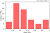 |
Fig. 19. Estimated progenitor masses (M⊙) for the 74 CSPNe in the HR diagram in Fig. 18. |
| In the text | |
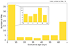 |
Fig. 20. Estimated evolutionary ages (kyr) for the 74 CSPNe in the HR diagram in Fig. 18. |
| In the text | |
|
Fig. 21. Image of a possible binary system in NGC 6720, showing the location of both the CSPN (with a cross) and the comoving companion. Image from the Aladin sky atlas (CDS). |
| In the text | |
|
Fig. 22. Image of a possible binary system in NGC 6781, showing the location of both the CSPN (with a cross) and the comoving companion. Image from the Aladin sky atlas (CDS). |
| In the text | |
|
Fig. 23. Image of a comoving system in PNG 030.8+03.4a, showing the location of both the CSPN (with a cross) and the companion. Image from the Aladin sky atlas (CDS). |
| In the text | |
|
Fig. 24. Image of a possible triple system in Fr 2–42, showing the location of the CSPN (with a cross) and the two comoving companions. Image from the Aladin sky atlas (CDS). |
| In the text | |
Current usage metrics show cumulative count of Article Views (full-text article views including HTML views, PDF and ePub downloads, according to the available data) and Abstracts Views on Vision4Press platform.
Data correspond to usage on the plateform after 2015. The current usage metrics is available 48-96 hours after online publication and is updated daily on week days.
Initial download of the metrics may take a while.