| Issue |
A&A
Volume 687, July 2024
|
|
|---|---|---|
| Article Number | A99 | |
| Number of page(s) | 13 | |
| Section | Interstellar and circumstellar matter | |
| DOI | https://doi.org/10.1051/0004-6361/202449751 | |
| Published online | 02 July 2024 | |
A study of two young multipolar planetary nebulae: Hen 2-73 and Hen 2-96
1
College of Geo-exploration Science and Technology, Jilin University,
Changchun
130012,
PR China
2
Institute of Integrated Information for Mineral Resources Prediction, Jilin University,
Changchun
130012,
PR China
e-mail: This email address is being protected from spambots. You need JavaScript enabled to view it.
3
Laboratory for Space Research, Faculty of Science, The University of Hong Kong,
Hong Kong,
China
e-mail: This email address is being protected from spambots. You need JavaScript enabled to view it.
4
Shekou International School Secondary Campus and ISS Asia Pacific Headquarters,
Shenzhen,
Guangdong Province,
PR China
5
Institute of Geochemistry, Chinese Academy of Sciences,
Guiyang
550081,
PR China
6
Deep Space Exploration Laboratory,
Beijing
100043,
PR China
7
Lunar Exploration and Space Engineering Centre, China National Space Administration,
Beijing
100190,
PR China
Received:
27
February
2024
Accepted:
30
April
2024
Abstract
We perform an infrared (IR) spectral and visible morphological study of two young planetary nebulae (YPNe) Hen 2-73 and Hen 2-96 using archival Spitzer Space Telescope and Hubble Space Telescope (HST) observations to understand their dust properties and nebular structures. High-resolution HST images of these nebulae show several bipolar lobes and ionised tori in the central regions of both objects. The presence of these multi-lobe structures suggests that the formation process of these nebulae is complex. To search for a possible link between the central sources and multipolar appearances of these objects, the Transiting Exoplanet Survey Satellite (TESS) observations are used to examine whether their central stars (CSs) exhibit periodic photometric variations. In the TESS observations, the CS light curve of Hen 2-96 shows a photometric variation with a period of 2.23 h. The IR spectra of these two YPNe suggest that the nebulae have mixed dust environments, which are associated with the presence of dense tori created by central binary interactions in these objects. Two three-dimensional models are constructed to study the complex nebular structures of the YPNe. These simulations suggest that the number of multipolar YPNe may be larger than observed. In addition, we analyse the spectral energy distributions of these nebulae to study their gas, dust, and photospheric components.
Key words: stars: AGB and post-AGB / planetary nebulae: general / ISM: structure / infrared: ISM
© The Authors 2024
 Open Access article, published by EDP Sciences, under the terms of the Creative Commons Attribution License (https://creativecommons.org/licenses/by/4.0), which permits unrestricted use, distribution, and reproduction in any medium, provided the original work is properly cited.
This article is published in open access under the Subscribe to Open model. This email address is being protected from spambots. You need JavaScript enabled to view it. to support open access publication.
1 Introduction
Planetary nebulae (PNe) are generally believed to form when the intermediate- and low-mass stars evolve to the end of their evolution. During the asymptotic giant branch (AGB) and post-AGB phases, the PN progenitors eject large amounts of material and form circumstellar envelopes around these sources. These materials are then gradually ionised by the central stars and eventually become PNe. As the PNe evolve, their shape changes over time, depending on the evolution of their central stars (Stanghellini et al. 2002), the densities of the environments surrounding the nebulae, and viewing angles to the PNe (Hsia et al. 2010, 2019, 2021). Among all PNe, multipolar nebulae are a unique type of PNe that usually exhibit two pairs or at least two pairs of axi-ally symmetrical structures (López et al. 1998; Manchado et al. 1996). Previous studies suggested that the vast majority of multipolar PNe are quite young (Sahai 2000; Kwok & Su 2005; Hsia et al. 2010, 2014, 2019). These results suggest that this type of nebulae plays a main role in the early stage of PN evolution (Hsia et al. 2014). The diversity of morphologies, complex structures, and chemical compositions of multipolar young PNe (YPNe) not only provides important information for the morphological evolution of PNe, but also helps us to understand the dust properties of these objects (Hsia et al. 2014).
In the past three decades, with the development of telescope equipment and high-dynamic-range CCD imaging technology, the properties of multipolar YPNe (morphology, ionised gas components, chemical compositions, and nebular structures) have been gradually studied in detail (Sahai 2000; Kwok & Su 2005; Hsia et al. 2010, 2014; Sahai et al. 2011, 2023; Leone et al. 2014; Hsia et al. 2019; Wen et al. 2023). Three quadrupo-lar (multipolar) PNe are first discovered in a survey of Galactic PN morphology and the shapes of these nebulae are inferred to be formed by precessing rotating stars (Manchado et al. 1996). Since then, more and more multipolar PNe have been discovered such as Hen 2-47 and M 1-37 (Sahai 2000), IRAS 21282+5050 (Hsia et al. 2019), NGC 6309 (Rubio et al. 2015), NGC 6644 (Hsia et al. 2010), and NGC 6881 (Kwok & Su 2005). The emergence of multipolar structures is suggested as a result of multiple outflow events separated by time or concurrent collimated outflows with different orientations (López et al. 1995; Hsia et al. 2014). While astronomers have proposed several scenarios to explain the formation of multipolar YPNe (López et al. 1995; García-Segura et al. 2006, 2010; Velázquez et al. 2012; Steffen et al. 2013), the exact mechanisms responsible for the shape of multi-lobed objects remain unclear. One possible cause for the presence of multiple lobes could be due to binary interactions in the core of the YPNe or precession of the rotating central star (CS) during the post-AGB or AGB phases (García-Segura 1997; García-Segura et al. 2010; Velázquez et al. 2012). Recent James Webb Space Telescope (JWST) observation of NGC 3132 reveals that the PN exhibits a multipolar morphology and has a triple star system (De Marco et al. 2022; Sahai et al. 2023). This result further supports the hypothesis that there may be a correlation between the multipolar appearance of the nebula and its central binary star (García-Segura et al. 2010; Velázquez et al. 2012).
The space-based all-sky photometry is a poweful tool that not only helps us discover the transits caused by Earth-size or giant planets orbiting solar-type stars (Holman et al. 2010; Batalha et al. 2011; Doyle et al. 2011; Lissauer et al. 2011; Welsh et al. 2012) and eclipsing binaries (Coughlin et al. 2011; Orosz et al. 2012; Thompson et al. 2012), but also detects binary CSs of PNe (CSPNe, Handler et al. 2013; De Marco et al. 2015; Aller et al. 2020; Jacoby et al. 2021; Rechy-García et al. 2022). The advantage of space photometric monitoring is that the observations are not affected by the Earth’s atmosphere and can carry out long-term continuous photometric measurements. Since the retirement of the Kepler space telescope, the current Transiting Exoplanet Survey Satellite (TESS) has become an excellent mission to search for new short-period binaries in the cores of all-sky PNe. A preliminary work using high-precision TESS photometry shows that 7 out of 8 CSPNe (~88%) exhibit significant periodic variations, which are attributed to the influence of binary CSs (Aller et al. 2020). However, these photometric variations may be contaminated by the other sources within the same photometric aperture (Aller et al. 2020). Further observations with better spatial resolution could confirm whether these CSPNe are binaries.
Hen 2-73 (PNG 296.3-03.0) and Hen 2-96 (PNG 309.0+00.8) are first discovered as Hα emission objects (Wray 1966). Henize (1967) further confirmed that they are true PNe according to their visible spectral characteristics. Both objects are originally classified as young bipolar nebulae (Sahai et al. 2011). Later, Stanghellini et al. (2016) classified Hen 2-73 as a point-symmetric (P) type nebula with a size of 5″.04×2″.11 because it reveals a point symmetry structure, while Hen 2-96 exhibits an irregular appearance (with a size of 4″.55×3″.68). Previous studies have revealed some properties of these two nebulae such as chemical abundances (Kaler 1970), distances (Maciel 1984), absolute fluxes (Acker et al. 1991), extinction coefficients (Tylenda 1992), and radial velocities (Durand et al. 1998). To understand the evolutionary status and mass distribution of the CSs of compact PNe, Moreno-Ibáñez et al. (2016) derive the CS masses and corresponding luminosities of the two objects to be ~0.567 M⊙ and 646 L⊙ for Hen 2–73 and ~0.567 M⊙ and 81 L⊙ for Hen 2-96, respectively, adopting the distances to these nebulae of 7.93 kpc (Hen 2-73) and 4.8 kpc (Hen 2-96). Although these two PNe may have bipolar features (Sahai et al. 2011) and some relevant properties have been reported previously, their shapes and complex structures have not been studied in detail.
In this study, we analyse the Hubble Space Telescope (HST) visible images, TESS photometry, and infrared (IR) spectral observations of two multipolar YPNe (Hen 2-73 and Hen 2-96) to study their morphology and properties and to search for the possible correlations between the central stars and the multi-lobed appearances of these YPNe. These mutlipolar structures have not been discovered before, possibly due to their low surface brightnesses. The two YPNe not only have mixed chemistry dust environments but also exhibit central ionised tori. A description of the visible imaging, photometry, and mid-IR (MIR) spectroscopic observations and their corresponding data reduction is presented in Sect. 2. In Sect. 3, we summarise the observed results of these nebulae. The photospheric, nebular, and dust properties of the two YPNe derived from the spectral energy distributions (SEDs) are given in Sect. 4. In Sect. 5, we use three-dimensional (3D) models to reconstruct the observations and study the multipolar appearance of these nebulae. Finally, a conclusion of our work is given in Sect. 6.
2 Observations and data reduction
2.1 High angular-resolution HST visible images
The visible imaging observations of Hen 2-73 and Hen 2-96 were taken from the Mikulski Archive for Space Telescopes (MAST). Both nebulae were imaged as part of program 11657 (PI: L. Stanghellini) using the Wide Field Camera 3 (WFC3) mounted on HST. The WFC3 provides a field-of-view (FOV) of 2′.7×2′.7 and a spatial resolution of 0″.04 per pixel, allowing detailed observations for the studied nebulae. Two broad-band (F350LP: λc = 5812 Å, Δλ = 4840 Å; F200LP: λc = 4895 Å, Δλ = 5680 Å) and one narrow-band [O III] (F502N: λc = 5012 Å, Δλ = 65 Å) filters were employed in the observations. The filters were used to capture the spatial structures and nebular features of these YPNe. The total exposure times of these objects ranged from 88 to 600 s, related to the brightness of the nebular structures observed in different filters.
To ensure the accuracy and reliability of the imaging results, we calibrated and processed the data using the IRAF STS-DAS package. The data reduction processes included flat-field calibration, bias correction, and cosmic-ray rejection, which were essential steps in reducing noise and other artefacts in the images. A summary of the HST WFC3 observations of these nebulae is given in Table 1. Processed colour composite and grey-scale F350LP images of these YPNe (Hen 2-73 and Hen 2-96) are shown in Figs. 1–3. These high-resolution images not only provide specific information on the spatial and structural distributions of the objects, but can also be used to study their dynamic evolution and physical properties.
2.2 TESS photometric observations
The TESS mission is an all-sky survey whose main purpose is to search for transiting exoplanets and monitor their variabilities. As of today, the TESS has already mapped more than 93% of the sky and observed 72 different sky sectors. The TESS has four cameras, each containing four 2K×2K CCDs. The camera provides a wide FOV of 24º×24º with an image resolution of 21″ pixel−1. As with Kepler mission, TESS’s continuous monitoring (~27 days) and high-precision observations provided a good opportunity to search for new binary central stars in the multipolar PNe.
We obtained the TESS photometric observations of Hen 2-73 and Hen 2-96 retrieved from MAST. These two YPNe were observed in the full frame images (FFIs) under a 200 s cadence mode. To obtain a series of CS photometric data of the nebulae, the 15×15 pixel2 cutouts (5′.3×5′.3) of FFIs were downloaded from MAST TESScut service (Brasseur et al. 2019) and then converted to the target pixel files (TPFs). Data reduction, photometry, and light curve creations of these objects were performed using Python Lightkurve v2.3.0 package (Lightkurve Collaboration 2018). Since the TPFs taken from raw FFIs were not processed for background subtraction, a basic median removal method and a RegressionCorrector task were used to remove the trends seen in the TPFs caused by spacecraft motion noise and scattered light. To minimise contamination from nearby sources, the aperture mask for each object was determined by manual inspection, which selected pixels that were least contaminated and showed strongest signal in the peri-odogram (Lightkurve Collaboration 2018). The CS light curves of Hen 2-73 and Hen 2-96 were then created from the calibrated TPFs using the to_lightcurve task in Lightkurve package. The remove_nans and remove_outliers tasks were employed to remove the data points with NaN fluxes and flux values above 5 times the standard deviation. Long term and low frequency trends were eliminated by applying a Savitzky-Golay filter. To search for possible periodicity in these YPNe, we performed a Lomb-Scargle periodogram analysis for the observed light curves, a method commonly used to detect periodic signals in non-uniformly spaced measurements. The phase-folded light curves of the objects corresponding to the period values found in the periodograms were made. The journal of the TESS photometric observations is summarised in Table 1 and the TPFs of these YPNe are shown in Fig. 4.
Given a large TESS image resolution of 21″ pixel−1, we should be cautious when analyzing the photometric signals of these nebulae obtained from the TESS mission due to potential contamination from nearby sources, which may lead to misinterpretation of the observed photometric variability (Higgins & Bell 2023; Pedersen & Bell 2023). From Fig. 4, we note that the photometric measurements of these nebulae are contaminated by a few sources with similar brightnesses to the CSPNe in the apertures, making it not easy to eliminate the contributions of nearby stars. To obtain the reliable localisation of observed variations in the TESS light curves and examine whether the variable signals originate from contaminant sources, the periodograms of these two PNe were first analysed using the TESS_Localize package (Higgins & Bell 2023). The TESS_Localize procedure could localise the position of a variable source on the sky better than one fifth of a TESS pixel (Higgins & Bell 2023). We adopted the same processes applied by Higgins & Bell (2023) and Gomes et al. (2024) to select the PNe that exhibited true photometric variability: (i) those with signal amplitudes larger than five times their uncertainties in the TESS_Localize procedure (Higgins & Bell 2023); and (ii) those with the “relative likelihood” (RL) parameter presented in the TESS_Localize procedure exceeds 90% (Higgins & Bell 2023; Gomes et al. 2024). Otherwise, the variations might come from other sources. After using the TESS_Localize method, we also performed additional visual inspections of the TPFs produced by TESS_Localize package to check whether the target positions match those of CSPNe.
Log of HST visible imaging and TESS photometric observations.
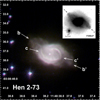 |
Fig. 1 HST colour-composite image of Hen 2-73 with various structures displayed in a logarithmic scale. The nebula is synthesised with [O III] (green), F200LP (blue), and F350LP (red) images. Two distinct lobe-like features (lobes b-b′ and c-c′) and a pair of faint bipolar lobe a-a′ are also labelled. The central star can be seen is the image. |
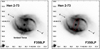 |
Fig. 2 Central region of Hen 2-73 shown in the grey-scaled F350LP image with a logarithmic scale. Left panel: image intensity is scaled to better show faint structures. The S-shaped lobe (c-c′) and a faint ionised torus roughly along the north-south direction can be seen. Right panel: same as on the left panel but marked with the tours feature (red dotted line). |
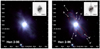 |
Fig. 3 Composite-colour HST images of PN Hen 2-96. Left panel: the image is created with F350LP (red), F200LP (blue), and [O III] (green) filters, respectively, and displayed in a logarithmic scale to show faint features. The insert (F350LP image) shows the central star and an ionised torus in central part of this nebula. Right panel: same as the left panel but labelled with individual structures. |
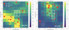 |
Fig. 4 Observed target pixel files (TPFs) of Hen 2-73 (left) and Hen 2-96 (right). The black crosses and coloured circles represent the locations of YPNe and the Gaia DR2 sources, respectively. The white shaded regions plotted on the TPFs are the aperture masks used to extract the fluxes of YPNe. The electron counts are displayed on a linear scale and the scale bars are shown at the right. Note that the photometric measurements of these YPNe may be contaminated by several sources inside the aperture masks. |
2.3 Infrared spectral observations
The IR spectra of these two YPNe were obtained from AKARI Infrared Camera (IRC) and Spitzer InfraRed Spectrograph (IRS) observations. For AKARI IRC spectroscopic measurements (Onaka et al. 2007), the observations of Hen 2-73 were performed under IRCZ4 mode with a spectral resolution ~100, covering a spectral range between 2.5 and 5.0 µm (Ohsawa et al. 2016). The IRCZ4 mode was designed for spectral measurements using IRC camera. The slit aperture used in the observations was 1′×3″. The total exposure on this nebula of IRC measurement was 355 sec. The data were processed and calibrated using IRC Spectroscopy Toolkit for Phase 3 data (version 20111121) to subtract dark and background emission, correct for flat-field and linearity, and calibrate wavelength and flux.
IRS low-to-medium resolution spectra of Hen 2-96 and Hen 2-73 were obtained through the program 50261 (PI: L. Stanghellini) between 2008 August 16 and 2009 April 03. The objects were observed with Long-High (LH), Short-Low (SL), and Short-High (SH) modules, which provide a total spectral coverage from 5.2 to 37.2 µm with spectral resolutions of 57– 600. The aperture sizes are l1″.1×22″.3, 3″.6×57″, and 4″.7×11″.3 for the LH, SL, and SH modules. Total exposures of the PNe varied between 40 s and 80 s, and the slits of spectroscopic observations for both nebulae were set to pass through their central regions. The IR spectra of these YPNe were reduced and calibrated using the Spitzer Science Centre (SSC) pipeline version s18.7. We employed the IRSCLEAN program to eliminate rogue pixels and then used the Spectroscopy Modelling Analysis and Reduction Tool (SMART) package to extract the spectra (Higdon et al. 2004). To obtain high signal-to-noise (S/N) spectral data for these YPNe, we combined the IRS observations with different exposures to create the final spectra of the studied nebula.
It is worth noting that the aperture size of the SL (3″.6×57″) and SH (4″.7×11″.3) modules is smaller than that of the LH (11″.1×22″.3) module, and the flux loss occurs in the SL and SH observations with smaller slit sizes. In order to correct this effect, we applied scaling correlations for the SL and SH observations of the two YPNe. The SL and SH measurements of these nebulae are scaled by the factors of 1.52 and 1.33 for Hen 2-73 and 1.21 and 1.08 for Hen 2-96, respectively, to suit the continuum intensities of overlapped parts of LH and SL/SH spectra.
The Spitzer and AKARI spectroscopic data of Hen 2-73 and Hen 2-96 have been presented by Ohsawa et al. (2016) and Stanghellini et al. (2012), but the dust chemical composition and characteristics of these YPNe have not been well studied. To better understand the dust properties of the two YPNe, we re-examined these spectra. A summary of Spitzer and AKARI observations of the objects is given in Table 2.
Summary of AKARI and Spitzer infrared spectroscopic observations.
Measurement results of structural features of Hen 2-73 and Hen 2-96.
3 Results
3.1 Visible morphology
3.1.1 Young planetary nebula with a multipolar shape – Hen 2-73 (PNG 296.3-03.0)
Although Sahai et al. (2011) have classified Hen 2-73 as a bipolar PN, the high-resolution HST image of this object (Fig. 1) shows that the nebula exhibits a multipolar shape extending roughly from southwest to northeast. This PN consists of three bipolar lobes (marked lobes a-a′, b-b′, and c-c′) and these lobe-like structures intersect approximately at the central part of the nebula. From Fig. 1, we can see that lobe c-c′ shows an approximate S-shaped appearance with western part twisting to the south and the eastern part twisting towards the north. The similar structure can be seen in some multipolar PNe such as Hen 2-313, IC 4634, and Kn 26 (Chong et al. 2012; Guerrero et al. 2013) and may be related to the precession of central binary interaction (Hsia et al. 2014; Kwok & Su 2005). Comparing to the two main lobes (lobes b-b′ and c-c′), the surface brightness of lobe a-a′ is relatively low and can only be distinguished by adjusting the contrast, as shown in the insert of Fig. 1. The shapes of lobe structures are measured by fitting their appearances in the images, allowing us to obtain their orientations and sizes. The sizes of these three lobes are 2″.35× 1″.13, 5″.35×2″.38, and 6″.58×2″. 16 for lobes c-c′, b-b′, and a-a′, respectively, and their corresponding position angles (PAs) are measured to be 63º±3º, 68º±2º, and 59º±2º. A summary of the measurement results is given in Table 3.
Furthermore, an ionised torus embedded in the waist of the twisted lobe c-c′ can be seen in the F350LP image of Hen 273 (Fig. 2). This torus structure has a size of 1″.20×0″.53 and is orientated at PA = 165°. Assuming that the shape of observed torus is due to a tilted circular projection, the tilt angle of this torus is approximately 64° (with 0° being the sky plane). Interestingly, we find that the orientation of lobe c-c′ (PA = 63°) is not perpendicular to the major axis of faint torus (PA = 165°). It is possible that the torus structure is not associated with lobe c-c′. The presence of these multi-lobed structures and ionised torus feature suggests that the formation process of this nebula is complex.
Precisely measuring the distances to PNe remains a challenge. Recent high-precision Gaia data are considered an ideal probe to obtain reliable distance scales (Stanghellini et al. 2020). Therefore, we use a Gaia distance to this PN of  kpc in this study (Bailer-Jones et al. 2021). Adopting that the distance of Hen 2-73 is 1.21 kpc (Bailer-Jones et al. 2021), the physical distance of lobe a-a′ is derived to be 0.039 sec θ pc (θ represents the tilt angle). Assuming that a mean expansion velocity of normal PNe is 42 km s−1 (Jacob et al. 2013), the kinematic age of this nebula is ~105 sec θ yr, indicating that Hen 2-73 is young (Sahai et al. 2011).
Results of our analysis for Hen 2-73 and Hen 2-96.
3.1.2 Young multipolar planetary nebula – Hen 2-96 (PNG 309.0+00.8)
The HST image of PN Hen 2-96 (Fig. 3) shows that this object has a bright, dense core and extends roughly from southwest to northeast. The angular dimension of this PN is 8″.58×5″.47, which is larger than earlier measurement of 4″.55×3″.68 (Stanghellini et al. 2016). As can be seen in Fig. 3, the nebula consists of four pairs of differently orientated lobes (marked as lobes d-d′, c-c′, b-b′, and a-a′) that roughly intersect at the central part of the nebula. The measured PAs of these four lobe-shaped features are 39°±4°, 47°±3°, 153°±3°, and 2°±4° for lobes a-a′, b-b′, c-c′, and d-d′, respectively. The angular extents of lobes a-a′, b-b′, c-c′, and d-d′ are about 8″.58×2″.16, 6″.68×2″.22, 2″.73×0″.77, and 2″.02×0″.68. The measured parameters of these structures (orientation angles and sizes) are also listed in Table 3.
Interestingly, the HST F350LP image of Hen 2-96 (the insert of Fig. 3) reveals a torus structure in the central part of this nebula. This torus feature is similar to that seen in Hen 2-73 (Fig. 2). The angular dimensions of this equatorial torus are 1″.06×(0″.46 orientated at PA = 138°. Assuming that the torus structure is caused by a tilted circle, the inclination angle of this ionised torus is derived to be 64° (with 0° being the sky plane). Further spectroscopic analysis of the ionised torus seen in Hen-96, as well as comparative studies of similar structures in other mul-tipolar PNe, can help us to gain a broader understanding of their formation mechanisms and evolution processes.
Adopting that the Gaia distance of Hen 2-96 is of 0.46 kpc (Bailer-Jones et al. 2021), the physical length of lobe a-a′ is 0.02 sec θ pc (where θ is the inclination angle). Assuming that a mean expansion velocity of this PN is 42 km s−1 (Jacob et al. 2013), the kinematic age of the nebula is estimated to be ~ 52 sec θ yr, which agrees with previous result that Hen 2-96 has a small nebular age (Sahai et al. 2011).
3.2 Potential photometric variations of the nebulae
After these detailed analyses of the TESS data, we determine that Hen 2-96 exhibits photometric variability but exclude Hen 2-73 because the TESS_Localize results of this PN show that the detected signals may originate from other sources. Table 4 lists the results of our analysis for these nebulae. The names of the sources are listed in Col. 1. Columns 2 and 3 give the period and amplitude of light curve variation. The time of minimum flux (T0) of the light curve modulation is given in Col. 4. Columns 5 and 6 give the classification of variability type based on the shape of phased curve and PN status adopted from the University of Hong Kong-Australian Astronomical Observatory-Strasbourg Observatory H-alpha (HASH) database (Parker et al. 2016). The RL values derived from TESS_Localize analysis is given in Col. 7. Figure 5 shows the TESS light curve (top panel), frequency-power spectrum (left panel), and phase-folded light curve obtained using the fitted period (right panel) of Hen 2-96. To better visualise the visibility of the phased light curve and estimate the amplitude variation of the object, the binned version of phase-folded light curve is also plotted on the right panel of Fig. 5. We summarise the photometric results of these two nebulae below.
3.2.1 Contaminated object – Hen 2-73
There is no information about photometric variability and spectral classification of the CS of this object in the literature. In the TESS frequency-power spectrum of this object, two prominent peaks at approximately 4.998 day−1 (4.8 h) and 9.997 day−1 (2.4 h) are identified. However, the TESS_localize analysis reveals that this nebula may be significantly contaminated by nearby sources with RL = 81.82%. There is few contamination from the star (Gaia DR3 5332582092820410368) with RL = 12.02% and another bright source (Gaia DR3 5332582092820404992) with RL = 2.74%. Further TPF analysis also reveals that the location of frequency source is slightly offset from this PN. These results suggest that Hen 2-73 seems unlikely to be the origin of the observed variability.
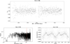 |
Fig. 5 TESS light curve of Hen 2-96 (top panel). Frequency power spectrum of TESS light curve (left panel). Phase folded (grey) and phase-binned (black) light curves of Hen 2-96 (right panel). The points in the phase-binned light curve (black) represent the average of data points in phase-folded light curve using the bin = 0.029 in phase. |
3.2.2 Photometric variation object – Hen 2-96
Although Hen 2-96 exhibits a striking multipolar appearance, the photometry and spectral classification of the CS in this nebula have not received attention in previous studies. The TESS peri-odogram of this object (left panel of Fig. 5) shows two notable features including a strong peak at 21.571 day−1 (1.11 h) and a weak peak at 10.786 days−1 (2.23 h). Our TESS_localize analysis shows that the analysed frequencies originate from this nebula (with RL ~ 98%). Further visual inspection of the TPF map also shows that the best-fit location of the target produced by TESS_localize overlaps with the position of the studied nebula, suggesting that the observed variation indeed originates from Hen 2-96. In addition, we note that the nebula is positioned very close to the edge of the aperture we set in the TPF map (see the right panel of Fig. 4), which may reduce the S/N of the measurement (Howell 1989) and affect the photometric variability of the observed object. To clarify and reduce the doubts caused by the chosen aperture, we adjust the aperture size to 2×2 pixel2 (where the position of the nebula is at the centre of the aperture) and then examine the photometric variation of the object. Similar to previous results, TESS_localize analysis reveals that the identified frequencies come from this object with RL = 97.12% and the frequency source location also overlaps on the analysed nebula after a visual inspection of the TPF map. These indicate that the offset position of Hen 2-96 has a rather small effect on the observed photometric variability.
The strong peak at 21.571 days−1 (1.11 h) does not show significant variation when we make a phase-folded light curve using this period, so the strong signal in the periodogram is most likely an alias. The CS phase light curve of this object folded with a period of 2.23 hr is shown in the right panel of Fig. 5. The curve with an amplitude of 0.13 percent (right panel of Fig. 5) presents double minima with different depths in each cycle and its shape is similar to the light curves of Th 3-12 (Jacoby et al. 2021) and β Lyrae (Kreiner et al. 1994; Kang 2010). The primary minimum appears to be about 2 times deeper than the secondary minimum. This variation is suspected to be caused by a semi-detached eclipsing binary with ellipsoidal components (Mennickent & Djurašević 2013).
Although Hen 2-96 exhibits periodic photometric variations, even though a RL value is about 98%, we cannot completely rule out the possibility that the observed variability is still contaminated by other stars surrounding the nebula. Additional high spatial resolution photometric monitoring is needed to help us clarify whether the variability comes from the CS of this object.
3.3 Dust properties of Hen 2-73 and Hen 2-96
To investigate the dust properties and chemical composition of the circumstellar medium surrounding Hen 2-73 and Hen 2-96, we examine the MIR spectra of these nebulae for the existence of silicate bands and unidentified infrared emission (UIE) features. Comparing with the Spitzer IRS spectrum of Hen 2-73, the AKARI IRC spectral data are observed with a smaller slit width (3″) and thus needed to be adjusted by a factor of 1.55 to suit the level of continuum emission at around 5.0 µm in the IRS spectrum. To emphasise unusual spectral features, we fit the dust continua of these nebulae by using the cubic polynomials and subtract them from the actual spectral data. The residual AKARI and Spitzer spectra of Hen 2-73 and Hen 2-96 are shown in Figs. 6 and 7, respectively.
As can be seen from Figs. 6 and 7, the residual IR spectra of the two YPNe are dominated by obvious forbidden lines including [Ar II] at 6.99 µm, [Ar III] at 8.99 µm, [Ne II] at 12.81 µm, [Ne III] at 15.56 µm, [S IV] at 10.51 µm, [S III] at 18.71 and 33.48 µm, and a prominent H 1 line at 12.37 µm. Hen 2-73 also exhibits more emission features such as [Mg IV] + [Ar VI] at around 4.49 µm, [Ar V] at 13.10 µm, [Ar III] at 21.83 µm, [Ne V] at 24.32 µm, and [O IV] at 25.87 µm. Additionally, the AKARI IRC spectrum of Hen 2-73 shows the HI and H2 features commonly found in typical PN spectra.
In addition to prominent forbidden lines, some strong UIE features at 6.2, 7.7, 8.6, 11.2/11.3, and 16.4 µm are observed in the IRS spectra of these two YPNe. Also present are weak UIE bands at 12.0, 11.8, 6.8, 5.7, 3.4, and 3.3 µm. Interestingly, the signatures of three main silicate complex features (23, 28, and 33 µm complexes) can also be detected in the IR spectroscopic measurements of Hen 2-73 and Hen 2-96 (Molster et al. 2002). These broad silicate bands lie in the wavelength range of 20– 35 µm and are detected for the first time in two YPNe. The dust composition characteristics mentioned above suggest the existence of a mixed dust environment in Hen 2-73 and Hen 2-96. The mixed-chemistry phenomena are associated with the presence of dense tori in these objects, which may be the product of central binary interactions (Guzman-Ramirez et al. 2011, 2014). Further high-spectral-resolution IR observations are required to understand the detail chemical compositions of these nebulae and 2D distributions of and their circumstellar environments.
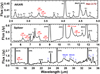 |
Fig. 6 Continua-subtracted spectra of Hen 2-73 with the spectral coverage from 2.5 to 5.0 µm (AKARI-IRC) and 5.0 to 36.0 µm (Spìtzer-IRS). Prominent forbidden emission, H2, and HI lines are labelled. The positions of UIE and silicate (Molster et al. 2002) bands are marked with red and blue lines, respectively. |
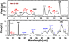 |
Fig. 7 Spitzer continuum-subtracted spectrum of Hen 2-96 in wavelength range of 5 to 36 µm. Obvious emissions and H2 line are labelled. The notations of UIE and crystalline silicate features are the same as Fig. 7. |
4 Spectral energy distribution
The SED has always been considered a powerful tool to help us study different components of various objects. To further understand the properties and nature of photospheric, dust, and ionised gas components of investigated nebulae, we set out to construct two individual SEDs for Hen 2-73 and Hen 2-96 (Fig. 8), covering wavelength range from radio to ultraviolet (UV). The visual Sloan Digital Sky Survey (SDSS) or Sloan z′, i′, r′, g′, u′ magnitudes of Hen 2-73 and Hen 2-96 are obtained from Henden et al. (2016) and Gaia Collaboration (2022), respectively. Extensive NIR and MIR photometric measurements are taken from Two Micron All Sky Survey (2MASS), Deep Near-Infrared Survey of the Southern Sky (DENIS), AKARI, Midcourse Space Experiment (MSX), Infrared Astronomical Satellite (IRAS), and Herschel point source catalogues. Additionally, some IR photometry of Hen 2-73 and Hen 2-96 measured from Wide-field Infrared Survey Explorer (WISE) archive are added together using the same methods presented in Hsia & Zhang (2014). The colour corrections of four WISE channels are performed using the calibration factors listed in Wright et al. (2010). We note that Hen 2-73 and Hen 2-96 are located in relatively dense environments. The photometric measurements of these nebulae may be contaminated by other sources in the field. After careful inspection, the photometry of both PNe are not contaminated by nearby objects from MIR to the radio bands. The visible photometric contamination of Hen 2-73 is <30% and NIR photometric contamination of Hen 2-96 is <15%. The photometric contamination from nearby sources on these two PNe is small and does not affect the main results. A journal of available photometric measurements is listed in Table 5.
As shown in Fig. 8, most of total fluxes emitted from these nebulae are mainly dominated by dust components in the IR range. We fitted the total emission intensities of Hen 2-73 and Hen 2-96 using the models composed of dust continuum and reddened photospheric emission (contributed from central core and ionised gaseous elements) described in Hsia et al. (2019). From Fig. 8, we can see that the relative proportions of these components of the YPNe can be clearly distinguished. For the dust continua shown in the SEDs, the distribution curves of these components are too broad to fit using a single element. Therefore, the observed curves of dust components of these nebulae are fitted by applying the DUSTY radiative transfer program (Ivezic et al. 1999). The dust chemistry of these two nebulae is assumed to be the mixtures of silicate, amorphous carbon, and graphite particles with a standard MRN size distribution (Mathis et al. 1977). The fiducial wavelengths and optical depths of the envelopes are adopted to be λ0 = 0.1 µm and τ = 0.3 for Hen 2-73 and λ0 = 0.7 µm and τ = 2.6 for Hen 2-96, respectively. In the SED fitting, although the fitting results do not fully reflect the actual status of these YPNe, we still give the best approximate fits to the observed data points.
Our best approximation results show that the effective temperatures of central cores are 100 000 ± 4000 K for Hen 2-73 and 55 000 ± 3000 K for Hen 2-96, which agree with previous results of 97 400 ± 3710 K for Hen 2-73 and 54 800 ± 3850 K for Hen 2-96 (Moreno-Ibáñez et al. 2016). The temperatures of dust components are derived to be 230 K and 180 K for Hen 2-73 and Hen 2-96. Adopting the same distances of 1.21 kpc for Hen 2-73 and 0.46 kpc for Hen 2-96 (Bailer-Jones et al. 2021), the total luminosities of Hen 2-73 and Hen 2-96 are ~1680 L⊙ and 2,160 L⊙. Due to some uncertainty in the effective temperatures of the central stars and the adopted distances of these objects, the derived luminosities of the two nebulae cannot be precisely determined, so the values are approximate estimates.
According to post-AGB evolutionary tracks proposed by Miller Bertolami (2016), the positions of Hen 2-73 and Hen 2-96 on the Hertzsprung-Russell diagram (central source temperatures and luminosities) imply that they have an evolutionary age of ⩾10 000 yr, corresponding to a core mass of ~0.528 M⊙. The evolutionary ages of these nebulae are larger than the observed kinematic ages derived earlier. The inconsistency between our observational results and the theoretical evolutionary tracks may be due to the fact that the visible nebular structures (for which we use to estimate the kinematic ages) originated from very late mass-loss stages, there is some uncertainty in the temperature and luminosity of these objects (Jones et al. 2019), the tracks are calculated for single stars rather than binary interactions (Jones et al. 2019), and these PNe belong to the post-red-giant-branch evolutions rather than the post-AGB systems. This scenario is associated with a common-envelope event that can shorten the evolution of the central star (Jones et al. 2022).
Assuming that the central source of Hen 2-96 is a binary star (§ 3.2), since the SED fit we constructed cannot distinguish the contribution of the cool companion, we cannot determine the physical parameters of this companion star through the current SED analysis. Obtaining high-dispersion UV and visible spectral measurements may help us to solve this issue (Feibelman 1997; Aller et al. 2015).
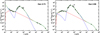 |
Fig. 8 Composited SEDs of Hen 2-73 and Hen 2-96 from 100 nm to 1 m. SDSS u′, g′, r′, i′, and t′ data are represented as open squares, DENIS results as filled triangles, the 2MASS measurements as open triangles, WISE photometry as open diamonds, IRAS results as filled circles, MSX photometric measurements as open rhombuses, AKARI results as asterisks, Herschel detections as filled diamonds, and available radio results as filled rhombuses. Note that the IRAS measurements at 100 µm are upper limits and light asterisks represent the uncertain AKARI detections. The dust emissions estimated by using the radiation-transfer simulation and nebular-continuum contributions are plotted as blue and red lines. The green curves denote the total fluxes estimated from all components. |
Photometry of Hen 2-73 and Hen 2-96.
5 3D structural simulation of Hen 2-73 and Hen 2-96
Based on the HST morphological study given in Sect. 3.1, Hen 2–73 and Hen 2-96 are considered to be young multipolar PNe. The intrinsic structure of this type of nebula is complex and difficult to analyse clearly. To better study and reproduce the complicated structures of these two YPNe, we employed the Shape software package (Steffen et al. 2011) to construct the 3D simulations of their structures and compare the corresponding 2D projections with observed images. Shape is a state-of-the-art, interactive 3D morphological and kinematic modelling software package designed for astrophysical research. The simulated structural parameters of these objects (the inclinations and sizes of the lobes) are taken from HST measurements. The surface brightness distribution of the observed lobe  is set to the cumulative emission intensity along the line-of-sight direction. By utilising the modelling capabilities of Shape software, we not only reproduce the complex 3D structures of Hen 2-73 and Hen 2-96 but provide useful information about their geometries. In these modelling simulations, hydrodynamic effects and excitation processes are not considered because we just want to study the 3D structural distributions of these nebulae and understand their 2D appearances.
Figure 9 shows the constructed models of these two YPNe, where Hen 2-73 has three pairs of bipolar lobes, while Hen 2-96 exhibits four lobe-shaped structures with closed tips. Gaussian blur is used for rendering in these models. Since some lobes of these nebulae exhibit a thin-shell appearance, the thin-shell geometry of the observed shell-like features is assumed to be 0″.1. Due to the lack of spectral results for each lobe of both YPNe, we cannot obtain a good estimate for the lobe lengths of these nebulae. Since some recent results suggest that partial multipolar YPNe have approximately equal lobe lengths (Guerrero & Manchado 1998; Rubio et al. 2015), we can assume that the visible lobe features of individual object in the models have the same length. Assuming that three bipolar lobes of Hen 2-73 are of equal length and the longest lobe a-a′ is located on the sky plane (with 90º being the line of sight), the derived inclinations of lobes b-b′ and c-c′ are 36º and 69º. For similar reason, lobe a-a′ is the longest lobe in Hen 2-96 and is therefore assumed to have an inclination of 0º (referred to the sky plane), the derived tilt angles are 39º, 71º, and 76º for lobes b-b′, c-c′, and d-d′, respectively. For Hen 2-96, lobes d-d′ and c-c′ are not clearly visible and do not exhibit a shell-like appearance as shown by the other two lobes (lobes b-b′ and a-a′). Therefore, we assigned a radial density-decreasing distribution to these two lobe-shaped structures. Although lobe b-b′ and lobe c-c′ of YPN Hen 2-73 are easily mixed together, these structures can still be reproduced in our model.
Measurements of several bipolar lobes and the parameters of model used are given in Table 6. Figure 9 also shows the comparison between simulation models and corresponding observation results of these two nebulae. From Fig. 9, our simulation models can reproduce most of the observed lobes compared to the structures seen in the HST images. In the investigation, we tried to make 3D model simulations of two YPNe based on the lobes observed in the observations, but different 3D model simulations may produce similar 2D appearances due to the degradation caused by projection. In fact, only position-velocity (PV) maps obtained through high-dispersion spectroscopy can help us to solve this degraded situation. Further kinematic data taken from high-spectral resolution observations are expected to improve this issue.
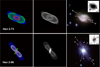 |
Fig. 9 Comparison of 3D model simulations and corresponding observed HST images of Hen 2-73 and Hen 2-96. Left row: 3D mesh models of Hen 2-73 and Hen 2-96. Note that the ionised torus elements in central regions of two YPNe are not constructed in the models. Middle row: the corresponding renderings of mesh model constructs. A Gaussian blur is used for rendering. Right row: composite-colour HST images of these nebulae for comparison. |
6 Conclusion
Over the past three decades, YPNe with multi-lobed appearances have been mis-categorised either as bipolar or as elliptical nebulae due to poor imaging measurements. Although more and more PNe with complex multipolar shapes have been unveiled via deep HST observations (Sahai 2000; Kwok & Su 2005; Kwok et al. 2010; Hsia et al. 2010, 2014, 2019; Wen et al. 2023), there are still a large number of multipolar nebulae that have not yet been identified, resulting in the true physical mechanisms behind the multipolar appearances being not clear. In current study, we perform an IR spectroscopic and visible morphological investigation of two multipolar YPNe (Hen 2-73 and Hen 2-96) to realise their dust properties and complicated multi-lobe appearances. The multipolar structures of these nebulae have not been studied before, probably because they are faint compared to main shells.
High-resolution HST images of the YPNe reveal several bipolar lobes and tori in the central regions of these objects. The emergence of the various structures shows that the formation process of these nebulae is complex. To investigate dust properties and chemical composition of the circumstellar medium surrounding Hen 2-73 and Hen 2-96, we examined the IR spectra of these nebulae for possible existence of distinctive spectral features. The residual IR spectra of these two YPNe show strong UIE bands at 6.2, 7.7, 8.6, 11.2/11.3, and 16.4 µm. Three main silicate complex bands (23, 28, and 33 µm complexes) are also detected for the first time in the IR spectra of these YPNe. The UIE and silicate signatures indicate the presence of mixed dust environments in Hen 2-73 and Hen 2-96, which are associated with the presence of dense tori created by central binary interactions in these objects.
To search for a possible link between the central sources and the shapes of these multipolar nebulae, the TESS observations are examined for the presence of photometric variability in their CSs. In the TESS photometric observations, the CS light curve of Hen 2-96 shows a photometric variation with a period of 2.23 hr, which is suspected to be caused by central binary. With this study, the TESS mission opens up a new possibility for the detection of central binaries in multipolar PNe.
Through analysis of nebular structures and the SED fits, we find that these two objects are relatively younger than typical PNe. Two 3D models of these YPNe with multi-lobe features are constructed to better understand their complex structures. The simulation models of these YPNe suggest that the number of multipolar YPNe may be larger than observed. With the help of high-resolution images together with high spectral-resolution spectroscopic observations, more multipolar nebulae such as Hen 2-73 and Hen 2-96 can be detected.
Modelling and observed parameters of the lobes for two young PNe.
Acknowledgements
We would like to thank the anonymous referee for his/her helpful comments that improved the manuscript. Part of the data used in this study were obtained from the Multi-mission Archive at the Space Telescope Science Institute (MAST). STScI is operated by the Association of Universities for Research in Astronomy, Inc., under NASA contract NAS5-26555. Support for MAST for non-HST data is provided by the NASA Office of Space Science via grant NAG5-7584 and by other grants and contracts. The Laboratory for Space Research was established by a grant from the University Development Fund of the University of Hong Kong. C.-H. Hsia thanks supports from the Hong Kong Research Grants Council for GRF research support under the grants 17326116 and 17300417. C.-H. Hsia thanks Q. A. Parker and HKU for provision of his research post. S. B. Wen and Y. Z. Wang were supported by National Key Research and Development Program of China (2022YFF0503102, 2022YFF0503100) and Granduate Innovation Fund of Jilin University (2024CX112).
References
- Acker, A., Stenholm, B., Tylenda, R., & Raytchev, B. 1991, A&AS, 90, 89 [NASA ADS] [Google Scholar]
- Aller, A., Montesinos, B., Miranda, L. F., et al. 2015, MNRAS, 448, 2822 [NASA ADS] [CrossRef] [Google Scholar]
- Aller, A., Lillo-Box, J., Jones, D., et al. 2020, A&A, 635, A128 [NASA ADS] [CrossRef] [EDP Sciences] [Google Scholar]
- Bailer-Jones, C. A. L., Rybizki, J., Fouesneau, M., Demleitner, M., & Andrae, R. 2021, AJ, 161, 147 [Google Scholar]
- Batalha, N. M., Borucki, W. J., Bryson, S. T., et al. 2011, ApJ, 729, 27 [Google Scholar]
- Brasseur, C. E., Phillip, C., Fleming, S. W., et al. 2019, Astrophysics Source Code Library, [record ascl:1905.007] [Google Scholar]
- Chong, S. N., Kwok, S., Imai, H., et al. 2012, ApJ, 760, 115 [NASA ADS] [CrossRef] [Google Scholar]
- Coughlin, J. L., López-Morales, M., Harrison, T. E., et al. 2011, AJ, 141, 78 [NASA ADS] [CrossRef] [Google Scholar]
- Cutri, R. M., Skrutskie, M. F., van DyK, S., et al. 2003, VizieR Online Data Catalogue: II/246 [Google Scholar]
- De Marco, O., Long, J., Jacoby, G. H., et al. 2015, MNRAS, 448, 3587 [Google Scholar]
- De Marco, O., Akashi, M., Akras, S., et al. 2022, Nat. Astron., 6, 1421 [Google Scholar]
- Doyle, L. R., Carter, J. A., Fabrycky, D. C., et al. 2011, Science, 333, 1602 [NASA ADS] [CrossRef] [Google Scholar]
- Durand, S., Acker A., & Zijlstra A. 1998, A&AS, 132, 13 [NASA ADS] [CrossRef] [EDP Sciences] [Google Scholar]
- Egan, M. P., Price, S. D., Kraemer, K. E., et al. 2003, The Midcourse Space Experiment Point Source Catalogue v2.3, Air Research Laboratory Technical Report AFRL-VS-TR-2003-1589 [Google Scholar]
- Elia, D., Molinari, S., Schisano, E., et al. 2017, MNRAS, 471, 100 [NASA ADS] [CrossRef] [Google Scholar]
- Feibelman, W. A. 1997, PASP, 109, 659 [NASA ADS] [CrossRef] [Google Scholar]
- Gaia Collaboration 2022, VizieR Online Data Catalogue: I/360 [Google Scholar]
- García-Segura, G. 1997, ApJ, 489, L189 [NASA ADS] [CrossRef] [Google Scholar]
- García-Segura, G. 2010, A&A, 520, A5 [NASA ADS] [CrossRef] [EDP Sciences] [Google Scholar]
- García-Segura, G., López, J. A., Steffen, W., et al. 2006, ApJ, 646, L61 [CrossRef] [Google Scholar]
- Gomes, R. L., Canto Martins, B. L., Fontinele, D. O., et al. 2024, ApJ, 961, 55 [NASA ADS] [CrossRef] [Google Scholar]
- Guerrero, M. A., & Manchado, A., 1998, ApJ, 508, 262 [NASA ADS] [CrossRef] [Google Scholar]
- Guerrero, M. A., Miranda, L. F., Ramos-Larios, G., et al. 2013, A&A, 551, A53 [NASA ADS] [CrossRef] [EDP Sciences] [Google Scholar]
- Guzman-Ramirez, L., Zijlstra, A. A., Níchuimín, R., et al. 2011, MNRAS, 414, 1667 [CrossRef] [Google Scholar]
- Guzman-Ramirez, L., Lagadec, E., Jones, D., et al. 2014, MNRAS, 441, 364 [NASA ADS] [CrossRef] [Google Scholar]
- Hale, C. L., McConnell, D., Thomson, A. J. M., et al. 2021, PASA, 38, e058 [NASA ADS] [CrossRef] [Google Scholar]
- Handler, G., Prinja, R. K., Urbaneja, M. A., et al. 2013, MNRAS, 430, 2923 [CrossRef] [Google Scholar]
- Henden, A. A., Templeton, M., Terrell, D., et al. 2016, VizieR On-line Data Catalog: II/336 [Google Scholar]
- Henize, K. G. 1967, ApJS, 14, 125 [NASA ADS] [CrossRef] [Google Scholar]
- Higdon, S. J. U., Devost, D., Higdon, J. L., et al., 2004, PASP, 116, 975 [NASA ADS] [CrossRef] [Google Scholar]
- Higgins, M. E., & Bell, K. J. 2023, AJ, 165, 141 [NASA ADS] [CrossRef] [Google Scholar]
- Holman, M. J., Fabrycky, D. C., Ragozzine, D., et al. 2010, Science, 330, 51 [Google Scholar]
- Howell, S. B. 1989, PASP, 101, 616 [CrossRef] [Google Scholar]
- Hsia, C.-H., & Zhang, Y. 2014, A&A, 563, A63 [NASA ADS] [CrossRef] [EDP Sciences] [Google Scholar]
- Hsia, C.-H., Kwok, S., Zhang, Y., et al. 2010, ApJ, 725, 173 [NASA ADS] [CrossRef] [Google Scholar]
- Hsia, C.-H., Chau, W., Zhang, Y., & Kwok, S. 2014, ApJ, 787, 25 [CrossRef] [Google Scholar]
- Hsia, C.-H., Zhang, Y., Kwok, S., & Chau, W. 2019, Ap&SS, 364, 32 [NASA ADS] [CrossRef] [Google Scholar]
- Hsia, C.-H., Zhang, Y., Sadjadi, S., et al. 2021, A&A, 655, A46 [NASA ADS] [CrossRef] [EDP Sciences] [Google Scholar]
- Irabor, T., Hoare, M. G., Burton, M., et al. 2023, MNRAS, 520, 1073 [NASA ADS] [CrossRef] [Google Scholar]
- Ishihara, D., Onaka, T., Kataza, H. et al. 2010, A&A, 514, A1 [NASA ADS] [CrossRef] [EDP Sciences] [Google Scholar]
- Ivezic, Z., Nenkova, M., & Elitzur M. 1999, DUSTY user manual, University of Kentucky internal report [Google Scholar]
- Jacob, R., Schönberner, D., & Steffen, M. 2013, A&A, 558, A78 [NASA ADS] [CrossRef] [EDP Sciences] [Google Scholar]
- Jacoby, G. H., Hillwig, T. C., Jones, D., et al. 2021, MNRAS, 506, 5223 [NASA ADS] [CrossRef] [Google Scholar]
- Jones, D., Boffin, H. M. J., Sowicka, P., et al. 2019, MNRAS, 482, L75 [Google Scholar]
- Jones, D., Munday, J., Corradi, R. L. M., et al. 2022, MNRAS, 510, 3102 [CrossRef] [Google Scholar]
- Kaler, J. B. 1970, ApJ, 160, 887 [NASA ADS] [CrossRef] [Google Scholar]
- Kang, Y.-W. 2010, J. Astron. Space Sci., 27, 75 [NASA ADS] [CrossRef] [Google Scholar]
- Kreiner, J. M., Pajdosz, G., Tremko, J., et al. 1994, A&A, 285, 459 [NASA ADS] [Google Scholar]
- Kwok, S., & Su, K. Y. L. 2005, ApJ, 635, 49 [Google Scholar]
- Kwok, S., Chong, S.-N., Hsia, C.-H., et al. 2010, ApJ, 708, 93 [NASA ADS] [CrossRef] [Google Scholar]
- Leone, F., Corradi, R. L. M., Martínez González, M. J., Asensio Ramos, A., & Manso Sainz, R. 2014, A&A, 563, A43 [NASA ADS] [CrossRef] [EDP Sciences] [Google Scholar]
- Lightkurve Collaboration (Cardoso, J. V. de M., et al.) 2018, Astrophysics Source Code Library, [record ascl:1812.013] [Google Scholar]
- Lissauer, J. J., Fabrycky, D. C., Ford, E. B., et al. 2011, Nature, 470, 53 [Google Scholar]
- López, J. A., Vázquez, R., & Rodriguez, L. F. 1995, ApJ, 455, L63 [Google Scholar]
- López, J. A., Meaburn, J., Bryce, M., et al. 1998, ApJ, 493, 803 [CrossRef] [Google Scholar]
- Maciel, W. J. 1984, A&A, 55, 253 [NASA ADS] [Google Scholar]
- Manchado, A., Stanghellini, L., & Guerrero, M. A. 1996, ApJ, 466, 95 [Google Scholar]
- Mathis, J. S., Rumpl, W., & Nordsieck, K. H. 1977, ApJ, 217, 425 [Google Scholar]
- Mennickent, R. E., & Djuraševic, G. 2013, MNRAS, 432, 799 [NASA ADS] [CrossRef] [Google Scholar]
- Miller Bertolami, M. M. 2016, A&A, 588, A25 [NASA ADS] [CrossRef] [EDP Sciences] [Google Scholar]
- Milne, D. K., & Aller, L. H. 1982, A&AS, 50, 209 [NASA ADS] [Google Scholar]
- Molster, F. J., Waters, L. B. F. M., & Tielens, A. G. G. M. 2002, A&A, 382, 222 [NASA ADS] [CrossRef] [EDP Sciences] [Google Scholar]
- Moreno-Ibáñez, M., Villaver, E., Shaw, R. A., & Stanghellini, L. 2016, A&A, 593, A29 [NASA ADS] [CrossRef] [EDP Sciences] [Google Scholar]
- Murphy, T., Sadler, E. M., Ekers, R. D., et al. 2010, MNRAS, 402, 2403 [Google Scholar]
- Ohsawa, R., Onaka, T., Sakon, I., Matsuura, M., & Kaneda, H. 2016, AJ, 151, 93 [NASA ADS] [CrossRef] [Google Scholar]
- Onaka, T., Matsuhara, H., Wada, T., et al. 2007, PASJ, 59, 401 [NASA ADS] [Google Scholar]
- Orosz, J. A., Welsh, W. F., Carter, J. A., et al. 2012, Science, 337, 1511 [Google Scholar]
- Parker, Q. A., Bojicic, I. S., & Frew, D. J., 2016, JPhCS, 728, 032008 [NASA ADS] [Google Scholar]
- Pedersen, M. G., & Bell, K. J. 2023, AJ, 165, 239 [NASA ADS] [CrossRef] [Google Scholar]
- Rechy-García, J. S., Toalá, J. A., Guerrero, M. A., et al. 2022, ApJ, 933, L24 [CrossRef] [Google Scholar]
- Retter, A., Leibowitz, E. M., & Naylor, T. 1999, MNRAS, 308, 140 [NASA ADS] [CrossRef] [Google Scholar]
- Rubio, G., Vázquez, R., Ramos-Larios, G., et al. 2015, MNRAS, 446, 1931 [CrossRef] [Google Scholar]
- Sahai, R. 2000, ApJ, 537, 43 [Google Scholar]
- Sahai, R., Morris, M. R., & Villar, G. G. 2011, AJ, 141, 134 [NASA ADS] [CrossRef] [Google Scholar]
- Sahai, R., Bujarrabal, V., Quintana-Lacaci, G., et al. 2023, ApJ, 943, 110 [NASA ADS] [CrossRef] [Google Scholar]
- Steffen, W., Koning, N., Esquivel, A., et al. 2013, MNRAS, 436, 470 [NASA ADS] [CrossRef] [Google Scholar]
- Stanghellini, L., Villaver, E., Manchado, A., & Guerrero, M. A. 2002, ApJ, 576, 285 [Google Scholar]
- Stanghellini, L., García-Hernández, D. A., García-Lario, P., et al., 2012, ApJ, 753, 172 [NASA ADS] [CrossRef] [Google Scholar]
- Stanghellini, L., Shaw, R. A., & Villaver, E. 2016, ApJ, 830, 33 [NASA ADS] [CrossRef] [Google Scholar]
- Stanghellini, L., Bucciarelli, B., Lattanzi, M. G., et al. 2020, ApJ, 889, 21 [NASA ADS] [CrossRef] [Google Scholar]
- Steffen, W., Koning, N., Wenger, S., Morisset, C., & Magnor, M. 2011, IEEE Trans. Vis. Comput. Graphics, 17, 454 [CrossRef] [Google Scholar]
- Stein, Y., Vollmer, B., Boch, T., et al. 2021, A&A, 655, A17 [NASA ADS] [CrossRef] [EDP Sciences] [Google Scholar]
- Tajitsu, A., & Tamura, S. 1998, AJ, 115, 1989 [NASA ADS] [CrossRef] [Google Scholar]
- Thompson, S. E., Everett, M., Mullally, F., et al. 2012, ApJ, 753, 86 [Google Scholar]
- Tylenda, R., Acker, A., Stenholm, B., & Koeppen J. 1992, A&AS, 95, 337 [NASA ADS] [Google Scholar]
- Velázquez, P. F., Raga, A. C., Riera, A., et al. 2012, MNRAS, 419, 3529 [CrossRef] [Google Scholar]
- Welsh, W. F., Orosz, J. A., Carter, J. A., et al. 2012, Nature, 481, 475 [Google Scholar]
- Wen, S.-B., Hsia, C.-H., Kang, X.-X., Chen, R., & Luo, T., 2023, Res. Astron. Astrophys., 23, 035018 [CrossRef] [Google Scholar]
- Wray, J. D. 1966, PhD thesis, Northwestern University, USA [Google Scholar]
- Wright, E. L., Eisenhardt, P. R. M., Mainzer, A. K., et al. 2010, AJ, 140, 1868 [Google Scholar]
All Tables
All Figures
|
Fig. 1 HST colour-composite image of Hen 2-73 with various structures displayed in a logarithmic scale. The nebula is synthesised with [O III] (green), F200LP (blue), and F350LP (red) images. Two distinct lobe-like features (lobes b-b′ and c-c′) and a pair of faint bipolar lobe a-a′ are also labelled. The central star can be seen is the image. |
| In the text | |
|
Fig. 2 Central region of Hen 2-73 shown in the grey-scaled F350LP image with a logarithmic scale. Left panel: image intensity is scaled to better show faint structures. The S-shaped lobe (c-c′) and a faint ionised torus roughly along the north-south direction can be seen. Right panel: same as on the left panel but marked with the tours feature (red dotted line). |
| In the text | |
|
Fig. 3 Composite-colour HST images of PN Hen 2-96. Left panel: the image is created with F350LP (red), F200LP (blue), and [O III] (green) filters, respectively, and displayed in a logarithmic scale to show faint features. The insert (F350LP image) shows the central star and an ionised torus in central part of this nebula. Right panel: same as the left panel but labelled with individual structures. |
| In the text | |
|
Fig. 4 Observed target pixel files (TPFs) of Hen 2-73 (left) and Hen 2-96 (right). The black crosses and coloured circles represent the locations of YPNe and the Gaia DR2 sources, respectively. The white shaded regions plotted on the TPFs are the aperture masks used to extract the fluxes of YPNe. The electron counts are displayed on a linear scale and the scale bars are shown at the right. Note that the photometric measurements of these YPNe may be contaminated by several sources inside the aperture masks. |
| In the text | |
|
Fig. 5 TESS light curve of Hen 2-96 (top panel). Frequency power spectrum of TESS light curve (left panel). Phase folded (grey) and phase-binned (black) light curves of Hen 2-96 (right panel). The points in the phase-binned light curve (black) represent the average of data points in phase-folded light curve using the bin = 0.029 in phase. |
| In the text | |
|
Fig. 6 Continua-subtracted spectra of Hen 2-73 with the spectral coverage from 2.5 to 5.0 µm (AKARI-IRC) and 5.0 to 36.0 µm (Spìtzer-IRS). Prominent forbidden emission, H2, and HI lines are labelled. The positions of UIE and silicate (Molster et al. 2002) bands are marked with red and blue lines, respectively. |
| In the text | |
|
Fig. 7 Spitzer continuum-subtracted spectrum of Hen 2-96 in wavelength range of 5 to 36 µm. Obvious emissions and H2 line are labelled. The notations of UIE and crystalline silicate features are the same as Fig. 7. |
| In the text | |
|
Fig. 8 Composited SEDs of Hen 2-73 and Hen 2-96 from 100 nm to 1 m. SDSS u′, g′, r′, i′, and t′ data are represented as open squares, DENIS results as filled triangles, the 2MASS measurements as open triangles, WISE photometry as open diamonds, IRAS results as filled circles, MSX photometric measurements as open rhombuses, AKARI results as asterisks, Herschel detections as filled diamonds, and available radio results as filled rhombuses. Note that the IRAS measurements at 100 µm are upper limits and light asterisks represent the uncertain AKARI detections. The dust emissions estimated by using the radiation-transfer simulation and nebular-continuum contributions are plotted as blue and red lines. The green curves denote the total fluxes estimated from all components. |
| In the text | |
|
Fig. 9 Comparison of 3D model simulations and corresponding observed HST images of Hen 2-73 and Hen 2-96. Left row: 3D mesh models of Hen 2-73 and Hen 2-96. Note that the ionised torus elements in central regions of two YPNe are not constructed in the models. Middle row: the corresponding renderings of mesh model constructs. A Gaussian blur is used for rendering. Right row: composite-colour HST images of these nebulae for comparison. |
| In the text | |
Current usage metrics show cumulative count of Article Views (full-text article views including HTML views, PDF and ePub downloads, according to the available data) and Abstracts Views on Vision4Press platform.
Data correspond to usage on the plateform after 2015. The current usage metrics is available 48-96 hours after online publication and is updated daily on week days.
Initial download of the metrics may take a while.