| Issue |
A&A
Volume 658, February 2022
|
|
|---|---|---|
| Article Number | A47 | |
| Number of page(s) | 15 | |
| Section | Stellar structure and evolution | |
| DOI | https://doi.org/10.1051/0004-6361/202141833 | |
| Published online | 01 February 2022 | |
Fundamental stellar parameters of benchmark stars from CHARA interferometry
II. Dwarf stars⋆
1
Landessternwarte, University of Heidelberg, Königstuhl 12, 69117 Heidelberg, Germany
e-mail: karovicova@uni-heidelberg.de
2
Sydney Institute for Astronomy (SIfA), School of Physics, University of Sydney, Sydney, NSW 2006, Australia
3
Stellar Astrophysics Centre (SAC), Department of Physics and Astronomy, Aarhus University, Ny Munkegade 120, 8000 Aarhus C, Denmark
4
Research School of Astronomy and Astrophysics, Australian National University, Canberra, ACT 2611, Australia
5
Center of Excellence for Astrophysics in Three Dimensions (ASTRO-3D), Stromlo, Australia
6
Institute for Astronomy, University of Hawai‘i, 2680 Woodlawn Drive, Honolulu, HI 96822, USA
Received:
3
July
2021
Accepted:
26
August
2021
Context. Stellar models applied to large stellar surveys of the Milky Way need to be properly tested against a sample of stars with highly reliable fundamental stellar parameters. We have established a programme aiming to deliver such a sample of stars.
Aims. Here we present new fundamental stellar parameters of nine dwarf stars that will be used as benchmark stars for large stellar surveys. One of these stars is the solar-twin 18 Sco, which is also one of the Gaia-ESO benchmarks. The goal is to reach a precision of 1% in effective temperature (Teff). This precision is important for accurate determinations of the full set of fundamental parameters and abundances of stars observed by the surveys.
Methods. We observed HD 131156 (ξ Boo), HD 146233 (18 Sco), HD 152391, HD 173701, HD 185395 (θ Cyg), HD 186408 (16 Cyg A), HD 186427 (16 Cyg B), HD 190360, and HD 207978 (15 Peg) using the high angular resolution optical interferometric instrument PAVO at the CHARA Array. We derived limb-darkening corrections from 3D model atmospheres and determined Teff directly from the Stefan–Boltzmann relation, with an iterative procedure to interpolate over tables of bolometric corrections. Surface gravities were estimated from comparisons to Dartmouth stellar evolution model tracks. We collected spectroscopic observations from the ELODIE spectrograph and estimated metallicities ([Fe/H]) from a 1D non-local thermodynamic equilibrium (NLTE) abundance analysis of unblended lines of neutral and singly ionised iron.
Results. For eight of the nine stars we measure the Teff ⪅ 1%, and for one star better than 2%. We determined the median uncertainties in log g and [Fe/H] as 0.015 dex and 0.05 dex, respectively.
Conclusions. This study presents updated fundamental stellar parameters of nine dwarf stars that can be used as a new set of benchmarks. All the fundamental stellar parameters were based on consistently combining interferometric observations, 3D limb-darkening modelling, and spectroscopic analysis. The next paper in this series will extend our sample to giants in the metal-rich range.
Key words: standards / techniques: interferometric / surveys / stars: general
Tables A.1.–A.9. are only available at the CDS via anonymous ftp to cdsarc.u-strasbg.fr (130.79.128.5) or via http://cdsarc.u-strasbg.fr/viz-bin/cat/J/A+A/658/A47
© ESO 2022
1. Introduction
Major efforts are underway to improve our understanding of stars, their populations, and thus the formation and evolution of our Galaxy. New instruments are enabling extensive surveys that allow us to explore the stellar content of the Milky Way in exquisite detail.
One of the latest and largest stellar surveys is being delivered by the Gaia satellite, which is creating a precise 3D map of more than a billion stars throughout our Galaxy (Gaia Collaboration 2016). Complementary spectroscopic surveys such as APOGEE (Allende Prieto et al. 2008), GALAH (De Silva et al. 2015), Gaia-ESO (Gilmore et al. 2012; Randich & Gilmore 2013), and the forthcoming 4MOST survey (de Jong et al. 2012) are providing the chemical compositions for a subset of Gaia stars. Overall, these large stellar surveys are helping us to improve our knowledge of the chemo-dynamical evolution of our Galaxy.
Our understanding of stellar structure and evolution requires accurate measurements of fundamental stellar parameters such as the effective temperature (Teff), surface gravity (log g), metallicity ([Fe/H]), and radius of the measured stars.
In most cases fundamental stellar parameters are determined using stellar spectroscopy. This unfortunately means that the parameters are determined indirectly and are model dependent. This negatively affects the accuracy of delivered results and consistency between surveys. Therefore, there is a great need for a set of reference stars called benchmark stars for which these parameters can be measured across a wide range of parameter space in a direct and survey-independent way.
Optical interferometry offers a suitable solution because it precisely measures the angular diameters of stars (Boyajian et al. 2012a,b, 2013; von Braun et al. 2014; Ligi et al. 2016; Baines et al. 2018; Rabus et al. 2019; Rains et al. 2020). The gold standard is then set by stars for which the effective temperature can be calculated directly from the measured angular diameter, θ, and bolometric flux, Fbol, according to the Stefan-Boltzmann law,
where σ is the Stefan-Boltzmann constant. If reliable measurements of angular diameters can be achieved, then the quality of the derived Teff will depend mainly on how well Fbol can be derived. We note that Teff is only weakly model-dependent via the adopted bolometric correction. For the stars analysed in this paper, a change of 2% in bolometric fluxes impacts Teff at the 30 K level, which is a 0.5% change. Additionally, the linear radius can be directly determined from the angular diameter given the parallax. Optical interferometry thus allows for the determination of Teff, in a direct and also survey-independent way. The stars with interferometrically measured angular diameters can then be used to rigorously test and improve the models that are used when deriving stellar parameters from spectroscopic surveys. Additionally, the stars can be used as fundamental benchmark stars to calibrate the characterisation of exoplanet host stars (Tayar et al. 2020). The correct determination of fundamental parameters of benchmark stars is therefore extremely important.
The Gaia-ESO survey used a sample of 34 stars that had been interferometrically measured as benchmarks (Jofré et al. 2014; Heiter et al. 2015). Although the angular diameters of the stars in this sample were observed using optical interferometry, and thus Teff was determined directly, the observations were collected from the literature from different instruments applying inconsistent limb-darkening corrections from various model atmosphere grids leading to an inhomogeneous dataset. Therefore, there is an urgent need to refine the measurement of the current sample. Moreover, a wider parameter space needs to be further explored and thus the sample of benchmarks needs to be expanded. The current sample is rather small; a larger sample is needed to robustly test stellar models.
We have been working to improve and expand the sample of benchmark stars via a consistent approach. We measured angular diameters with the highest possible precision using a single state-of-the-art interferometric instrument, applying consistent limb-darkening corrections determined from the best available stellar models. We resolved discrepancies between the spectroscopic, photometric, and interferometric Teff of the metal-poor stars in the original Gaia-ESO benchmark sample (Karovicova et al. 2018). Recently, we presented the fundamental stellar parameters of a new and updated set of ten metal-poor benchmark stars (Karovicova et al. 2020). Here we present a second set of benchmarks from our sample, nine dwarf stars, where the fundamental stellar parameters of the stars were delivered applying the same methods as in the first sample.
2. Observations
2.1. Science targets
We observed nine dwarf stars as a part of our programme which aims to deliver stars that can be used as benchmarks. The dwarf stars will be added to the first set of metal-poor stars from this programme in Karovicova et al. (2020). The parameters of the dwarf stars are listed in Table 1 and are shown in Fig. 1.
Stellar parameters.
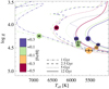 |
Fig. 1. Stellar parameters of our programme stars, colour-coded by metallicity, compared to theoretical Dartmouth isochrones of different ages (line styles) and with metallicities [Fe/H] = +0.2, 0.0 and −0.5 (colours). Formal 1σ uncertainties are shown by the error bars. The symbol size is proportional to the angular diameter of each star. |
Two stars (HD 152391 and HD 207978) were interferometrically observed for the first time. One of the stars (HD 146233 (18 Sco)) is a current Gaia-ESO benchmark star. The star was interferometrically observed by Bazot et al. (2011) and Boyajian et al. (2012a). The Gaia-ESO benchmark sample adopted the angular diameter measured by Bazot et al. (2011); however, the measurement is in stark disagreement with the measurement by Boyajian et al. (2012a), which is inconsistent with the status of solar twin. We are revising it here to confirm the angular diameter value of Bazot et al. (2011). We discuss these previous measurements, and compare them with our new measurements in Sect. 4.3. Five of the other eight stars (HD 131156, HD 173701, HD 185395, HD 186408, and HD 186427) have been proposed as future benchmarks by Heiter et al. (2015).
Three targets are in multiple systems (HD 131156, HD 186408, and HD 186427). HD 131156 (ξ Boo A) has a K5V companion which is more than 5 arcsec away (Mason et al. 2001) and makes a negligible contribution to the flux in Precision Astronomical Visible Observations (PAVO) instrument, as evidenced by the lack of a short baseline deficit in V2 in Fig. 2. HD 186408 (16 Cyg A) is separated by approximately 40 arcsec from HD 186427 (16 Cyg B), and both stars are observed as single objects by PAVO. HD 186408 is itself a close binary, separated by approximately 3 arcsec from a faint red dwarf companion (Raghavan et al. 2006). As for HD 131156, this companion makes a negligible contribution to the flux.
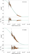 |
Fig. 2. Squared visibility vs. spatial frequency for HD 131156 and HD 146233. The HD number is noted in the upper right corner of each plot. The raw error bars were scaled to the reduced χ2 before the final fitting. For HD 131156 the reduced χ2 = 4.7 and for HD 146233 χ2 = 3.7. The grey dots are the individual PAVO measurements in each wavelength channel. For clarity, the weighted averages of the PAVO measurements are shown as red circles. The green line shows the fitted limb-darkened model to the PAVO data, with the light grey shaded region indicating the 1σ uncertainties. Lower panel: residuals from the fit. |
The metallicities of our nine dwarf stars range between −0.5 and +0.2 dex. HD 173701 and HD 190360 both appear metal rich for their age in Fig. 1. We have integrated their kinematics over the past 3 Gyr using the MWPotential14 model within the galpy python package (Bovy 2015) and find that the mean guiding radius of these stars to be 6.9 and 7.1 kpc, respectively. This is broadly consistent with their higher metallicity and not atypical of outward migrations for ∼10−11 Gyr stars (Minchev et al. 2018).
2.2. Interferometric observations and data reduction
Our interferometric observations were collected using the PAVO interferometric instrument (Ireland et al. 2008) at the Center for High Angular Resolution Astronomy (CHARA) array at Mt. Wilson Observatory, California (ten Brummelaar et al. 2005). PAVO is operating as a pupil-plane beam combiner in optical wavelengths between ∼630−880 nm. The limiting magnitude of the observed targets is R ∼ 7.5, which can be slightly extended up to R ∼ 8 if the weather conditions allow. The CHARA Array offers baselines up to 330 m, thus making it the longest available baselines in the optical wavelengths worldwide.
The stars were observed using baselines between 65.91 m and 330.7 m. We collected the observations between 2013 July 6 and 2016 August 13. Additionally, several of our targets were previously observed with PAVO between 2009 and 2012. We included these observations in our study so that all data could be analysed consistently. In particular, our treatment of limb-darkening differs from the previous studies. The previously published data include one night of observations of 18 Sco (Bazot et al. 2011), which we supplement with three nights of new observations, as well as the observations of HD 173701 (Huber et al. 2012), 16 Cyg A and B, and θ Cyg (White et al. 2013). Table 2 summarises the dates of all observations, telescope configurations, and the baselines, B (distance between telescopes). The data were reduced with the PAVO reduction software. The PAVO data reduction software has been used in multiple studies (e.g. Bazot et al. 2011; Derekas et al. 2011; Huber et al. 2012; Maestro et al. 2013) and it has been well tested, especially for single baseline squared visibility (V2) observations.
Interferometric observations – dwarfs.
The data reduction software allows the application of several visibility corrections. In particular, a coherence time (t0) correction based on a ratio of coherent and incoherent visibility estimators may be used to correct visibility losses. The t0 correction can introduce biases, and we have chosen not to use it. We note, however, that this correction was used in the study of 16 Cyg A and B, and θ Cyg by White et al. (2013). Here we carry out a fresh data reduction for each target. We analyse the data consistently with the rest of the data in this study.
In comparison to the previous studies, we changed the wavelength range we used, including all 38 channels, which range between 630 and 880 nm. The previous studies only used the central 23 channels between 650 and 800 nm because the channels at either end may be unreliable. However, after a careful investigation of our data, we found no such concerns, and so we included the full range in our analysis.
Immediately before and after the science targets a set of calibrating stars was observed allowing us to monitor the interferometric transfer function. These calibrating stars were selected from a catalogue of CHARA calibrators and from the HIPPARCOS catalogue (ESA 1997). Calibrators were selected to be unresolved or nearly unresolved sources that were located close on sky to our targets. We determined the angular diameters of the calibrators using the V − K relation of Boyajian et al. (2014), and corrected for limb-darkening to determine the uniform disc diameter in the R band. We used V band magnitudes from the Tycho-2 catalogue (Høg et al. 2000) and converted into the Johnson system using the calibration by Bessell (2000). The K band magnitudes were selected from the Two Micron All Sky Survey (2MASS; Skrutskie et al. 2006). The reddening was estimated from the dust map of Green et al. (2015), and the reddening law of O’Donnell (1994) was applied. The relative uncertainty on calibrator diameters was set to 5% (Boyajian et al. 2014). This uncertainty covers both the uncertainty on the calibrator diameters as well as the reddening. The absolute uncertainty on the wavelength scale was set to 5 nm. We checked all calibrators for binarity. According to Gaia DR2, the proper motion anomaly (Kervella et al. 2019), the phot_bp_rp_excess_factor (Evans et al. 2018), and the renormalised unit weight error (RUWE; Belokurov et al. 2020) all suggest that none of our calibrators has a companion that is large enough to affect our interferometric measurements or estimated calibrator sizes. For the calibrators, we used uniform disc angular sizes in the R band. We found that using high-order limb-darkening coefficients to estimate of the calibrator sizes has a negligible impact (∼0.3%), which is substantially smaller than our 5% uncertainty in the calibrator diameters. All the calibrating stars, their spectral types, magnitudes in the V and R band, their expected angular diameters, and the corresponding science targets are summarised in Table 3.
Calibrator stars used for interferometric observations – dwarfs.
3. Methods
Our methodology for delivering the stellar parameters is largely consistent with that in Karovicova et al. (2020) so the results are homogeneous. The connection between the interferometric, photometric and spectroscopic analysis is described in detail therein. Here we repeat some key points, and point out differences and updates.
3.1. Modelling of limb-darkened angular diameters
Observations in the first lobe of the visibility function are degenerate between the angular diameter and limb-darkening. A limb-darkened disc appears much the same as a slightly smaller uniformly illuminated disc at these spatial frequencies. To determine the true angular diameters of our targets we therefore rely on stellar atmosphere models to infer the amount of limb-darkening present.
Limb-darkening laws are used to parametrise the intensity profile with a small number of coefficients. It is common in interferometric studies to use a linear limb-darkening law (Schwarzschild 1906),
where μ = cos(γ) and γ is the angle between the line of sight and the normal to a given point on the stellar surface, and u is the linear limb-darkening coefficient. However, the linear law does not adequately reproduce the intensity profiles of observations (e.g. Klinglesmith & Sobieski 1970) and of models (e.g. Claret & Bloemen 2011). For this study, as for our previous studies (Karovicova et al. 2018, 2020), we therefore adopted the four-term non-linear limb-darkening law of Claret (2000),
where ak is the limb-darkening coefficient.
We derived the limb-darkening coefficients for our targets from the STAGGER grid of ab initio 3D hydrodynamic stellar model atmosphere simulations (Magic et al. 2013). We use these models because they have been shown to better reproduce the solar limb-darkening than both theoretical and semi-empirical 1D hydrostatic models (Pereira et al. 2013); therefore, we expect them to give better overall results in general. For each model in the grid and for each of the 38 wavelength channels of PAVO we fitted Eq. (3) to the μ-dependent synthetic fluxes calculated by Magic et al. (2015). We then linearly interpolated within this grid to find the limb-darkening coefficients for each star, which are given in Tables A.1.–A.9, available at the CDS. In the appendix we include one table for one of the stars as an example.
The fringe visibility is related to the source intensity distribution by a Fourier transform. Following the fringe visibility for a generalised polynomial limb-darkening law (Quirrenbach et al. 1996), the fringe visibility for the four-term non-linear law is
![$$ \begin{aligned} V =&\left(\frac{1-\sum a_k}{2}+\sum _k\frac{2a_k}{k+4}\right)^{-1}\nonumber \\&\times \left[\left(1-\sum _k a_k\right)\frac{J_1(x)}{x}+\sum _k a_k 2^{k/4}\Gamma \left(\frac{k}{4}+1\right)\frac{J_{k/4+1}(x)}{x^{k/4+1}} \right], \end{aligned} $$](/articles/aa/full_html/2022/02/aa41833-21/aa41833-21-eq4.gif)
where x = πBθλ−1, with B the projected baseline, θ the angular diameter, Γ(z) is the gamma function, and Jn(x) is the nth-order Bessel function of the first kind. The quantity Bλ−1 is the spatial frequency. We fitted this equation to our observed visibilities to determine the angular diameters of our targets. We determined the uncertainties in our measurements by Monte Carlo simulations that incorporated the uncertainties in the visibility measurements, the wavelength calibration (5 nm), calibrator sizes (5%), and the limb-darkening coefficients. The correlations between wavelength channels are taken into account by bootstrapping. The raw error bars are scaled by χ2 before the final fitting. The squared visibilities versus spatial frequencies along with the residuals from the fit are shown in in Figs. 2–6.
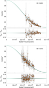 |
Fig. 3. Squared visibility vs. spatial frequency for HD 152391 and HD 173701. Lower panel: residuals from the fit. The error bars are scaled to the reduced χ2. For HD 152391 the reduced χ2 = 2.4 and for HD 173701 χ2 = 2.2. All lines and symbols are the same as in Fig. 2. |
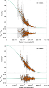 |
Fig. 4. Squared visibility vs. spatial frequency for HD 185395 and HD 186408. Lower panel: residuals from the fit. The error bars have been scaled to the reduced χ2. For HD 185395 the reduced χ2 = 18.4 and for HD 186408 χ2 = 5.8. All lines and symbols are the same as in Fig. 2. |
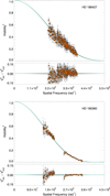 |
Fig. 5. Squared visibility vs. spatial frequency for HD 186427 and HD 190360. Lower panel: residuals from the fit. The error bars are scaled to the reduced χ2. For HD 186427 the reduced χ2 = 8.1 and for HD 190360 χ2 = 1.6. All lines and symbols are the same as in Fig. 2. |
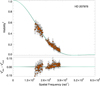 |
Fig. 6. Squared visibility vs. spatial frequency for HD 207978. Lower panel: residuals from the fit. The error bars are scaled to the reduced χ2. The reduced χ2 = 6.8. All lines and symbols are the same as in Fig. 2. |
While our recommended stellar parameters are based on angular diameters determined in this way, for ease of comparison with other studies where the treatment of limb-darkening may be different, we also calculated angular diameters for a uniformly illuminated disc model, that is, without limb-darkening. Additionally, we determined the angular diameters for a linearly limb-darkened disc model using coefficients determined from the grid of Claret & Bloemen (2011), as had been done for the previous studies using PAVO data that we reanalyse here. These values are given in Table 4. We note that the angular diameters are on average 0.8% smaller than, but still within 1σ of, the values obtained in the previous studies. These differences are due to the updated analysis, as described in Sect. 2.2. The limb-darkened diameters based on the STAGGER-grid are listed in Table 5.
Angular diameters and linear limb-darkening coefficients.
Observed (θLD) and derived (Fbol, M, L, R) stellar parameters.
3.2. Bolometric flux
The bolometric fluxes and associated uncertainties were derived with the exact same procedure described in Karovicova et al. (2020). Briefly, we adopted an iterative procedure to interpolate over the tables of bolometric corrections1 of Casagrande & VandenBerg (2014, 2018). We used HIPPARCOSHp and Tycho2 BTVT magnitudes for all stars, and 2MASS JHKS only if they had quality flag ‘A’. Reddening was assumed to be zero for our science targets as they are all located between ∼10 and 30 pc from us, and thus well within the Local Bubble. The adopted bolometric corrections are listed in Table 6.
Bolometric corrections.
We note that our uncertainties in bolometric fluxes do not take into account possible inaccuracies in model fluxes. Comparison with absolute spectrophotometry indicates that by using multiple bands, bolometric fluxes from the CALSPEC library can be recovered at the one percent level for FG stars (Casagrande & VandenBerg 2018). However, our sample comprises cooler stars, for which the performance of our bolometric corrections is much less tested (see e.g. discussions in White et al. 2018; Rains et al. 2021; Tayar et al. 2020). Encouragingly, comparison with the absolute spectrophotometry of a few GK subgiants in White et al. (2018) indicates that reliable fluxes can still be obtained from our bolometric corrections. As pointed out earlier, it should also be kept in mind that a given percentage change in bolometric flux carries a four times smaller percentage change in effective temperatures.
3.3. Spectroscopic analysis
We measured a set of unblended Fe I and Fe II lines from high-resolution R ≈ 42 000 spectra from the ELODIE archive (Moultaka et al. 2004). We used a pipeline based on the Spectroscopy Made Easy (SME) code (Piskunov & Valenti 2017), together with MARCS model atmospheres (Gustafsson et al. 2008) and non-LTE corrections from Amarsi et al. (2016).
We performed a differential abundance analysis by a comparison to measurements on a solar spectrum recorded with the same spectrograph from reflected light off the Moon. These differential measurements remove zero-level uncertainties in the reference oscillator strengths, and ensure that metallicity measurements are relative to the Sun with no significant zero-point uncertainty. Our iron abundance estimates are based on an outlier-resistant mean with 3σ clipping. We also estimate abundances separately for Fe I and Fe II; comparing these two measurements offers an independent check on the accuracy of our stellar parameters as systematic errors are expected to yield deviations from ionisation equilibrium. In addition to our statistical uncertainties, we also estimated the systematic errors on the metallicity. These estimates were computed from the effect of uncertainties in each of the stellar parameters on the metallicity measurements, and then combined in quadrature.
3.4. Stellar evolution models
We determined stellar masses using the Dartmouth stellar evolution tracks (Dotter et al. 2008), which cover a wide range of ages and metallicities. We used solar-scaled models with [α/Fe] = 0 since the stars investigated in this work are thin-disc stars with no discernible α-enhancement at low metallicity. We performed the fitting using the ELLI package2 (Lin et al. 2018), which uses a Bayesian framework to estimate mass and age from our estimates of Teff, logL/L⊙, and [Fe/H]. Errors on these parameters are assumed to be symmetric and independent. This code samples the posterior distribution using a Markov chain Monte Carlo (MCMC) method; we estimate the mass and its uncertainty from the mean and standard deviation of this distribution. The surface gravity is computed directly from this estimate on the form
where G is the gravitational constant and ϖ the parallax.
4. Results and discussion
4.1. Recommended stellar parameters
We present fundamental stellar parameters and angular diameters for a set of nine dwarf stars: HD 131156 (ξ Boo), HD 146233 (18 Sco), HD 152391, HD 173701, HD 185395 (θ Cyg), HD 186408 (16 Cyg A), HD 186427 (16 Cyg B), HD 190360, and HD 207978 (15 Peg). We present the stars as a new set of benchmark stars. We estimate radius and mass from measurements of θLD, Fbol, and parallax for all nine stars. All these values, along with luminosity, are summarised in Table 5. The final fundamental stellar parameters of Teff, log g, and [Fe/H] are presented in Table 7, and are discussed below.
Derived stellar parameters (Teff, log g, [Fe/H]).
4.2. Uncertainties
The final uncertainties in Teff are due, independently, to the uncertainties in the bolometric flux and to the uncertainties in the angular diameter. The contributions from each are shown in Table 8, where they have been computed by artificially setting the uncertainties from the other measurement to zero. For clarity the dominating uncertainty is highlighted in boldface.
Uncertainties in Teff and how they propagate from the underlying measurements.
It should be noted that in the final Teff error estimates, we propagate the statistical measurement uncertainties in log g and [Fe/H] from the isochrone fitting and spectroscopic analysis, which were folded into the uncertainties in the angular diameters. The median uncertainties in log g and [Fe/H] across our sample of stars are 0.015 dex and 0.05 dex, respectively (Table 7).
The uncertainties in Teff are less than 50−60 K (or less than 1%) for all but two stars in our sample. For one of these the uncertainty is equal to 1%. For the remaining star the uncertainty in Teff is higher than 1%, however, still low (1.7%). The uncertainty for these two stars is dominated by errors in the bolometric flux. Errors in Teff resulting from uncertainties in the limb-darkened angular diameters are at most 40 K, with a median of just 29 K (0.5%). The only star in our dwarf sample for which we report Teff uncertainties larger than 1% (1.7%) is HD 131156. As already mentioned, the Teff uncertainty is dominated by the uncertainty in the bolometric flux; therefore, the Fbol value for this star requires refinement before the star fully meets the set requirements for the Teff precision. As mentioned previously, the desired precision requested by the spectroscopic teams such as Gaia-ESO or GALAH is around 1% (or around 40−60 K).
4.3. Comparison with angular diameter values in the literature
In total, seven of the stars have been previously interferometrically observed. We present the first published angular diameters for two stars: HD 152391 and HD 207978. For some of the stars we conducted new observations and for all the stars we carried out fresh data reduction and analysis of the data. For all the stars we applied our updated analysis and updated treatment of limb-darkening modelling. Table 9 lists our measurements of angular diameters θLD together with values reported in the literature. We compare these values in Fig. 7.
Previous angular diameters.
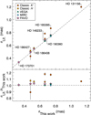 |
Fig. 7. Comparison of limb-darkened angular diameters from the literature with measurements from this work. Symbols correspond to the beam combiner used for the literature measurement: CHARA Classic in the K′ and H band (orange and yellow squares, respectively), VEGA in the H band (green triangles), MIRC in the H band (light blue circle), and PAVO in visible (pink stars). |
HD 131156 (ξ Boo). We observed this star and measured the angular diameter as θLD = 1.124 ± 0.009 mas. This star was previously interferometrically observed by Boyajian et al. (2012a) using the Classic instrument in the K′ band at the CHARA array who reported θLD = 1.196 ± 0.014 mas. We note that the difference of the θLD value in comparison with the previous study is almost 4σ over the quoted uncertainties. We discuss possible reasons for the difference between our measurement using the PAVO instrument and the measurement from the Classic instrument below. This star was suggested as a possible benchmark star in Heiter et al. (2015); therefore, we included it in our observing sample.
HD 146233 (18 Sco). We measured angular diameter of this star as θLD = 0.663 ± 0.005 mas. 18 Sco was previously observed by Bazot et al. (2011) with the same interferometric instrument, PAVO. However, the data were collected on a single night and so are potentially susceptible to calibration errors. The published angular diameter from that night is θLD = 0.676 ± 0.006 mas. 18 Sco is a Gaia-ESO benchmark and the value of θLD reported by Bazot et al. (2011) was adopted by the Gaia-ESO survey (Jofré et al. 2015). The values of θLD differ by 1.4σ. This difference is due, in part, to the additional observations included in our measurement, but also because of the different limb-darkening correction. Additional interferometric observations of this star were conducted by Boyajian et al. (2012a), who observed the star using the Classic instrument at the CHARA array and reported θLD = 0.780 ± 0.017 mas. Here the difference between the values is over 6σ. We again discuss the possible reasons in more detail below.
HD 152391. This star was interferometrically observed for the first time. We report the angular diameter of θLD = 0.477 ± 0.007 mas.
HD 173701. For this star we report θLD = 0.329 ± 0.005 mas. The data were previously analysed by Huber et al. (2012), who reported θLD = 0.332 ± 0.006 mas. Huber et al. (2012) fitted a linearly limb-darkened disc model to the data, determining the limb-darkening coefficient from the grid calculated by Claret & Bloemen (2011) from 1D ATLAS models. For consistency, we carried out new data reduction and re-analysed the data with limb-darkening coefficients from 3D model atmospheres and using a higher-order limb-darkening model. In this case, the angular diameters are in agreement. This star was suggested as a possible benchmark star in Heiter et al. (2015).
HD 185395 (θ Cyg). This star was previously observed several times with various interferometric instruments. For this star we report θLD = 0.737 ± 0.006 mas. We re-visited data observed by White et al. (2013) who found a value of θLD = 0.754 ± 0.009 mas. The differences between our value of θLD and the value determined by White et al. (2013) can be explained by a combination of our new reduction of the data and the different treatment of limb-darkening. We note that our value is in agreement with the measurement made by White et al. (2013) using the MIRC beam combiner at CHARA (θLD = 0.739 ± 0.015 mas), which operates in the H band where limb-darkening is weaker. Our value is slightly smaller than the value obtained at visible wavelengths with the VEGA beam combiner at CHARA by Ligi et al. (2016), who found θLD = 0.749 ± 0.007 mas. All these values are significantly smaller than the value obtained with the Classic in the K′ band of θLD = 0.861 ± 0.015 mas (Boyajian et al. 2012a). This star was also suggested as a possible benchmark star.
HD 186408 (16 Cyg A). For this star we report θLD = 0.525 ± 0.004 mas. Here, we carried out a new data reduction and re-analysis of data observed with the PAVO instrument by White et al. (2013), who reported θLD = 0.539 ± 0.006 mas. Again, this difference can be attributed to our new reduction and the updated limb-darkening treatment. We discuss the matter in more detail below. Boyajian et al. (2013) published observations of this star using the Classic instrument in the H band and found a larger value, θLD = 0.554 ± 0.011 mas. This star is listed as a candidate for a benchmark (Heiter et al. 2015).
HD 186427 (16 Cyg B). For this star we report θLD = 0.479 ± 0.004 mas. We re-visited PAVO data observed by White et al. (2013). The previous reported value of θLD was θLD = 0.490 ± 0.006 mas. CHARA Classic observations have been made in the K′ band by Baines et al. (2008) and in the H band by Boyajian et al. (2013); the authors reported angular diameters of θLD = 0.426 ± 0.056 mas and θLD = 0.513 ± 0.012 mas, respectively. Since the star was suggested as a possible candidate as a benchmark star, for consistency the data was freshly reduced, re-analysed, and the limb-darkening coefficients from 3D model atmospheres using a higher-order limb-darkening model were applied.
HD 190360. We observed the star and measured angular diameter as θLD = 0.663 ± 0.005 mas. Our value agrees with the value, θLD = 0.662 ± 0.006 mas, found with the VEGA instrument by Ligi et al. (2016). This star was also previously observed by Baines et al. (2008) using the CHARA Classic instrument in the K′ band, who found θLD = 0.698 ± 0.019 mas. Possible reasons for this difference are discussed below.
HD 207978 (15 Peg). The last star in our dwarf sample has not been previously observed interferometrically. We determined the angular diameter to be θLD = 0.542 ± 0.005 mas.
As we have noted, the differences between previous PAVO diameters and our values based on the same data are attributable to a combination of our fresh data reduction and changes to the limb-darkening correction. Both of these changes contribute almost equally to our diameters being an average of 2% smaller than the previous PAVO values.
Most of the changes in our new data reduction had only a small impact on the result. These changes include making different choices around outlier rejection based on S/N and other metrics, new calculations of calibrator sizes, and using more of the observed wavelength channels. The most significant impact results from our choice not to use the t0 correction, as described in Sect. 2.2. The effect of these data reduction changes is reflected in the limb-darkened angular diameters given in Table 4, which used linear limb-darkening coefficients determined in the same way as in the previous studies.
The change to the limb-darkening treatment makes up the remainder of the difference. The previous PAVO studies used linear limb-darkening coefficients calculated from 1D ATLAS model atmospheres in Cousins R band, either by Claret (2000) or Claret & Bloemen (2011). Two different methods of determining the linear coefficient were used by Claret & Bloemen (2011), a simple least-squares (LS) fit to the intensity profile, and a flux-conserving (FC) fit. The previous PAVO studies adopted the average of the values determined by these methods, and used the difference as an estimate of the uncertainty. The R band value was used across all wavelength channels between 650 and 800 nm.
As noted in Sect. 3.1, the linear limb-darkening law is a poor fit to both observations and models of centre-to-limb intensity profiles. This is so because the intensity drops sharply close to the limb. As a result, a simple linear LS fit to the intensity profile will produce a stronger limb-darkening across the vast majority of the stellar disc than is appropriate. The FC fit of Claret & Bloemen (2011) takes account of this by altering the slope of the fit to ensure that the integrated flux over the stellar disc is conserved.
An alternate way to determine an appropriate linear coefficient was recently used by Rains et al. (2020). Their equivalent linear coefficient (ELC) produces the same first sidelobe height in the interferometric visibility function as higher-order models or observations.
The differences between these coefficients are illustrated by Fig. 8, where we show model and observed linear limb-darkening coefficients for the Sun as a function of wavelength. The ELCs that correspond to the four-term non-linear limb-darkening law coefficients we use in this work agree well with ELCs that match the solar observations of Neckel & Labs (1994). By comparison, the linear coefficients determined by Claret & Bloemen (2011) from 1D ATLAS models and by Magic et al. (2015) from the 3D STAGGER grid imply stronger limb-darkening, with the coefficients determined by a LS fit giving the worst results. Additionally, the previous practice of applying the R band value to all wavelength channels also resulted in a bias towards stronger limb-darkening. The previous studies therefore used limb-darkening corrections that were too strong, resulting in angular diameters that were too large.
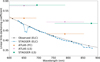 |
Fig. 8. Solar linear limb-darkening coefficients as a function of wavelength. Black points, joined by a dashed line to guide the eye, show the equivalent linear coefficients (ELCs) calculated from the observations of Neckel & Labs (1994). Blue points, joined by a solid blue line, show the ELCs calculated from the 3D STAGGER solar model (Magic et al. 2015) in each of the 38 wavelength channels of PAVO. Triangles show linear coefficients calculated by Claret & Bloemen (2011) from 1D ATLAS models in Cousins R and I bands. They used two different methods, flux-conserving (FC) and least-squares (LS) fits to the models, indicated by upward orange triangles and downward pink triangles, respectively. Green squares show the linear coefficients calculated using a LS fit from the STAGGER model in Johnson R and I bands by Magic et al. (2015). The error bars show the full width at half maximum of the respective bandpasses. See text for a discussion of the different methods of determining the coefficients. |
Even larger differences are found between our measurements and several of those made with the Classic beam combiner, particularly in the K′ band. Such differences have been noted previously (e.g. Casagrande et al. 2014; Karovicova et al. 2018; White et al. 2018), and can arise from several factors, including the target star not being resolved well enough.
4.4. Spectroscopic analysis
We show in Fig. 9 that our abundance determinations for lines of neutral and singly ionised iron are in good agreement: the median and median absolute deviation are 0.00 ± 0.02 dex. As errors in stellar parameters have different impact on lines of neutral and singly ionised iron, these measurements offer an independent test of the quality of our stellar parameters. We estimate that an error in Teff of 100 K would affect the abundances measured from neutral iron lines compared to lines ionised by 0.1 dex; conversely, an error in log g of 0.10 dex would have a corresponding effect of 0.05 dex.
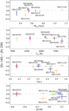 |
Fig. 9. Deviations from ionisation equilibrium (i.e. the difference between the abundances determined from lines of neutral and ionised iron) as a function of the measured stellar parameters. Vertical and horizontal lines represent the combined uncertainties from the two measurements. Stars are colour-coded according to metallicity, as in Fig. 1. |
We find that only three out of nine stars exhibit a deviation from ionisation equilibrium greater than their estimated measurement errors, and only significantly so for two stars. We note that these are also the coolest stars in our sample, indicating that the error may be related to our spectroscopic modelling rather than potential errors in the stellar parameters. Crucially, there is no apparent correlation with the angular diameters.
4.5. Comparison with asteroseismology
Stellar radii may also be precisely determined from asteroseismic measurements. Such measurements exist for several of our targets; here we briefly compare asteroseismic radii for these stars with our values from interferometry.
The most direct method of determining radii from asteroseismology is to exploit scaling relations for two global asteroseismic parameters, the frequency of maximum power, νmax, and the large frequency separation, Δν (e.g. Kallinger et al. 2010). The value of νmax is empirically observed to scale as (Brown et al. 1991; Kjeldsen & Bedding 1995)
and Δν scales as (Ulrich 1986)
By measuring Δν and νmax, and given Teff, combining these two relations directly gives the mass and radius. A more rigorous method is to model the stars in detail using individual oscillation frequencies and other measurements as observational constraints. Detailed modelling allows other stellar properties to be constrained, such as age, in addition to the mass and radius.
Four of our targets were observed during the original Kepler mission. Of these, three (HD 173701, HD 186408, and HD 186427) are included in the Kepler LEGACY sample (Lund et al. 2017; Silva Aguirre et al. 2017). We used the measurements of νmax and Δν by Lund et al. (2017) for these stars to calculate scaling relation radii. Detailed asteroseismic modelling for the LEGACY sample was conducted by Silva Aguirre et al. (2017) using several modelling pipelines. For simplicity, here we only use the values derived from the BASTA pipeline to illustrate typical modelling results.
The fourth Kepler star, HD 185395, was studied by Guzik et al. (2016). We use the νmax and Δν values they measured to determine the scaling relation radius. Guzik et al. (2016) used the interferometric radius as a constraint, along with the oscillation frequencies, in their detailed modelling of this star. While this means that a fair comparison of the modelled radius with the interferometric radius cannot be made, we include their modelled radius determined from YREC models (Demarque et al. 2008) to illustrate the stark difference between the scaling relation and modelled radius for this star.
Figure 10 compares the scaling relation and modelling asteroseismic radii with our interferometric radii. As can be expected, the radii determined from the scaling relations do not agree as closely with the interferometric radii as the radii from detailed modelling. The biggest disagreement between interferometry and the scaling relations can be seen for HD 185395. The apparent failure of the scaling relation in this case can be attributed to it being applied to a star that is more than 1000 K hotter than the Sun. White et al. (2011) highlighted that the Δν scaling relation, while working well in models, requires a temperature-dependent correction when applying it to stars significantly different to the Sun. Applying such a correction here would substantially improve the agreement for this star.
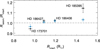 |
Fig. 10. Comparison of radii determined from asteroseismic scaling relations (black) and modelling (blue) with interferometric radii from this work. |
In contrast, the agreement between the modelled radii and the interferometric radii is generally good for all stars, although differences remain. Huber et al. (2012) were unable to reconcile differences between their interferometric and asteroseismic observations, and stellar models for HD 173701. They noted that a higher effective temperature would help to bring better agreement. Despite our revised angular diameter being slightly smaller than the value determined by Huber et al. (2012), we also find a lower bolometric flux than they adopted, such that the effective temperature remains unchanged. Tension between asteroseismic and interferometric results such as this, however, may be of value for calibrating the free parameters of stellar models, such as the mixing length parameter (e.g. Hjørringgaard et al. 2017; Joyce & Chaboyer 2018).
Finally, we note that HD 146233 has also been observed asteroseismically by Bazot et al. (2011). However, because a measurement of νmax was not reported by Bazot et al. (2011) we have not been able to calculate a scaling relation radius to compare with our measurement. Modelling of this star by Bazot et al. (2018) also used the interferometric measurement as a constraint, and subsequently did not report radius as an output of the modelling.
5. Conclusions
The goal of this study is to extend a sample of stars with highly accurate and reliable fundamental stellar parameters that are used as benchmark stars for large stellar surveys. This is the second in a series of papers with this scientific goal. Here we determined fundamental stellar parameters of nine dwarf benchmark stars HD 131156 (ξ Boo A), HD 146233 (18 Sco), HD 152391, HD 173701, HD 185395 (θ Cyg), HD 186408 (16 Cyg A), HD 186427 (16 Cyg B), HD 190360, and HD 207978 (15 Peg).
We observed the stars using the high angular resolution instrument PAVO at the CHARA array in order to measure the angular diameters of the stars. We observed the stars over various nights and with various baseline configurations with the aim of resolving the targets close to the first null of the visibility curve. We estimated the limb-darkening diameters using the 3D radiation-hydrodynamical model atmospheres in the STAGGER-grid. We determined the Teff directly from from the Stefan-Boltzmann relation together with photometric modelling of bolometric flux. Bolometric fluxes were computed from multi-band photometry, interpolating iteratively on a grid of synthetic stellar fluxes to ensure consistency with the final adopted stellar parameters.
Based on high-resolution spectroscopy, we determined [Fe/H], and we used isochrone fitting to derive mass and parallax measurements to constrain the absolute luminosity. After iterative refinement we derived the final fundamental parameters of Teff, log g, and [Fe/H]. One of the stars from the sample HD 146233 (18 Sco) is listed as a Gaia-ESO benchmark star. There has been a strong disagreement between two interferometric values determined by Bazot et al. (2011) and Boyajian et al. (2012a). We resolved the discrepancies and updated the fundamental stellar parameters for this important solar twin. We also determined stellar parameters for five stars previously proposed as benchmarks in Heiter et al. (2015).
For eight stars we reached the required precision of ⪅1% in the Teff. Only one star (HD 131156) showed a somewhat larger Teff uncertainty, which is still less than 2%. The Teff uncertainty for this star is dominated by errors in the bolometric flux. For surface gravity log g we reached a median precision of just 0.015 dex and 0.05 dex in metallicity [Fe/H]. We showed that the updated limb-darkening approach gives slightly different results in comparison to previous interferometric measurements derived using the same instrument, justifying the revisit of previous measurements.
The following paper in this series will extend our sample to giants in the metal-rich range. These benchmark stars will be used as a proper scale for stellar models applied to spectroscopic surveys. Therefore, the precision we have been able to achieve is crucial for the correct determination of the atmospheric parameters of the stars observed by the surveys where the scaled stellar models are applied. Properly scaled models will allow us to better understand the physics of stars in our Galaxy.
Acknowledgments
I.K. acknowledges the German Deutsche Forschungsgemeinschaft, DFG project number KA4055 and the European Science Foundation – GREAT Gaia Research for European Astronomy Training. This work is based upon observations obtained with the Georgia State University Center for High Angular Resolution Astronomy Array at Mount Wilson Observatory. The CHARA Array is supported by the National Science Foundation under Grants No. AST-1211929 and AST-1411654. Institutional support has been provided from the GSU College of Arts and Sciences and the GSU Office of the Vice President for Research and Economic Development. Funding for the Stellar Astrophysics Centre is provided by The Danish National Research Foundation. L.C. is the recipient of the ARC Future Fellowship FT160100402. T.N. acknowledges funding from the Australian Research Council (grant DP150100250). Parts of this research were conducted by the Australian Research Council Centre of Excellence for All Sky Astrophysics in 3 Dimensions (ASTRO 3D), through project number CE170100013. D.H. acknowledges support from the Alfred P. Sloan Foundation, the National Aeronautics and Space Administration (80NSSC19K0379), and the National Science Foundation (AST-1717000). This work is based on spectral data retrieved from the ELODIE archive at Observatoire de Haute-Provence (OHP).
References
- Allende Prieto, C., Majewski, S. R., Schiavon, R., et al. 2008, Astron. Nachr., 329, 1018 [NASA ADS] [CrossRef] [Google Scholar]
- Amarsi, A. M., Lind, K., Asplund, M., Barklem, P. S., & Collet, R. 2016, MNRAS, 463, 1518 [NASA ADS] [CrossRef] [Google Scholar]
- Baines, E. K., McAlister, H. A., ten Brummelaar, T. A., et al. 2008, ApJ, 680, 728 [NASA ADS] [CrossRef] [Google Scholar]
- Baines, E. K., Armstrong, J. T., Schmitt, H. R., et al. 2018, AJ, 155, 30 [Google Scholar]
- Bazot, M., Ireland, M. J., Huber, D., et al. 2011, A&A, 526, L4 [NASA ADS] [CrossRef] [EDP Sciences] [Google Scholar]
- Bazot, M., Creevey, O., Christensen-Dalsgaard, J., & Meléndez, J. 2018, A&A, 619, A172 [NASA ADS] [CrossRef] [EDP Sciences] [Google Scholar]
- Belokurov, V., Penoyre, Z., Oh, S., et al. 2020, MNRAS, 496, 1922 [Google Scholar]
- Bessell, M. S. 2000, PASP, 112, 961 [Google Scholar]
- Bovy, J. 2015, ApJS, 216, 29 [NASA ADS] [CrossRef] [Google Scholar]
- Boyajian, T. S., McAlister, H. A., van Belle, G., et al. 2012a, ApJ, 746, 101 [Google Scholar]
- Boyajian, T. S., von Braun, K., van Belle, G., et al. 2012b, ApJ, 757, 112 [Google Scholar]
- Boyajian, T. S., von Braun, K., van Belle, G., et al. 2013, ApJ, 771, 40 [Google Scholar]
- Boyajian, T. S., van Belle, G., & von Braun, K. 2014, AJ, 147, 47 [Google Scholar]
- Brown, T. M., Gilliland, R. L., Noyes, R. W., & Ramsey, L. W. 1991, ApJ, 368, 599 [Google Scholar]
- Casagrande, L., & VandenBerg, D. A. 2014, MNRAS, 444, 392 [Google Scholar]
- Casagrande, L., & VandenBerg, D. A. 2018, MNRAS, 475, 5023 [Google Scholar]
- Casagrande, L., Portinari, L., Glass, I. S., et al. 2014, MNRAS, 439, 2060 [Google Scholar]
- Claret, A. 2000, A&A, 363, 1081 [NASA ADS] [Google Scholar]
- Claret, A., & Bloemen, S. 2011, A&A, 529, A75 [NASA ADS] [CrossRef] [EDP Sciences] [Google Scholar]
- de Jong, R. S., Bellido-Tirado, O., Chiappini, C., et al. 2012, in Ground-based and Airborne Instrumentation for Astronomy IV, eds. I. S. McLean, S. K. Ramsay, & H. Takami, SPIE Conf. Ser., 8446, 84460T [NASA ADS] [Google Scholar]
- De Silva, G. M., Freeman, K. C., Bland-Hawthorn, J., et al. 2015, MNRAS, 449, 2604 [NASA ADS] [CrossRef] [Google Scholar]
- Demarque, P., Guenther, D. B., Li, L. H., Mazumdar, A., & Straka, C. W. 2008, Ap&SS, 316, 31 [NASA ADS] [CrossRef] [Google Scholar]
- Derekas, A., Kiss, L. L., Borkovits, T., et al. 2011, Science, 332, 216 [NASA ADS] [CrossRef] [Google Scholar]
- Dotter, A., Chaboyer, B., Jevremović, D., et al. 2008, ApJS, 178, 89 [Google Scholar]
- ESA 1997, The Hipparcos and Tycho Catalogues, 1200 [Google Scholar]
- Evans, D. W., Riello, M., De Angeli, F., et al. 2018, A&A, 616, A4 [NASA ADS] [CrossRef] [EDP Sciences] [Google Scholar]
- Gaia Collaboration (Prusti, T., et al.) 2016, A&A, 595, A1 [NASA ADS] [CrossRef] [EDP Sciences] [Google Scholar]
- Gilmore, G., Randich, S., Asplund, M., et al. 2012, The Messenger, 147, 25 [NASA ADS] [Google Scholar]
- Green, G. M., Schlafly, E. F., Finkbeiner, D. P., et al. 2015, ApJ, 810, 25 [Google Scholar]
- Gustafsson, B., Edvardsson, B., Eriksson, K., et al. 2008, A&A, 486, 951 [NASA ADS] [CrossRef] [EDP Sciences] [Google Scholar]
- Guzik, J. A., Houdek, G., Chaplin, W. J., et al. 2016, ApJ, 831, 17 [NASA ADS] [CrossRef] [Google Scholar]
- Heiter, U., Jofré, P., Gustafsson, B., et al. 2015, A&A, 582, A49 [NASA ADS] [CrossRef] [EDP Sciences] [Google Scholar]
- Hjørringgaard, J. G., Silva Aguirre, V., White, T. R., et al. 2017, MNRAS, 464, 3713 [CrossRef] [Google Scholar]
- Høg, E., Fabricius, C., Makarov, V. V., et al. 2000, A&A, 355, L27 [Google Scholar]
- Huber, D., Ireland, M. J., Bedding, T. R., et al. 2012, ApJ, 760, 32 [Google Scholar]
- Ireland, M. J., Mérand, A., ten Brummelaar, T. A., et al. 2008, Proc. SPIE, 7013, 701324 [NASA ADS] [CrossRef] [Google Scholar]
- Jofré, P., Heiter, U., Soubiran, C., et al. 2014, A&A, 564, A133 [NASA ADS] [CrossRef] [EDP Sciences] [Google Scholar]
- Jofré, P., Heiter, U., Soubiran, C., et al. 2015, A&A, 582, A81 [Google Scholar]
- Joyce, M., & Chaboyer, B. 2018, ApJ, 864, 99 [NASA ADS] [CrossRef] [Google Scholar]
- Kallinger, T., Weiss, W. W., Barban, C., et al. 2010, A&A, 509, A77 [CrossRef] [EDP Sciences] [Google Scholar]
- Karovicova, I., White, T. R., Nordlander, T., et al. 2018, MNRAS, 475, L81 [Google Scholar]
- Karovicova, I., White, T. R., Nordlander, T., et al. 2020, A&A, 640, A25 [NASA ADS] [CrossRef] [EDP Sciences] [Google Scholar]
- Kervella, P., Arenou, F., Mignard, F., & Thévenin, F. 2019, A&A, 623, A72 [NASA ADS] [CrossRef] [EDP Sciences] [Google Scholar]
- Kjeldsen, H., & Bedding, T. R. 1995, A&A, 293, 87 [NASA ADS] [Google Scholar]
- Klinglesmith, D. A., & Sobieski, S. 1970, AJ, 75, 175 [Google Scholar]
- Ligi, R., Creevey, O., Mourard, D., et al. 2016, A&A, 586, A94 [NASA ADS] [CrossRef] [EDP Sciences] [Google Scholar]
- Lin, J., Dotter, A., Ting, Y.-S., & Asplund, M. 2018, MNRAS, 477, 2966 [CrossRef] [Google Scholar]
- Lund, M. N., Silva Aguirre, V., Davies, G. R., et al. 2017, ApJ, 835, 172 [Google Scholar]
- Maestro, V., Che, X., Huber, D., et al. 2013, MNRAS, 434, 1321 [NASA ADS] [CrossRef] [Google Scholar]
- Magic, Z., Collet, R., Asplund, M., et al. 2013, A&A, 557, A26 [NASA ADS] [CrossRef] [EDP Sciences] [Google Scholar]
- Magic, Z., Chiavassa, A., Collet, R., & Asplund, M. 2015, A&A, 573, A90 [NASA ADS] [CrossRef] [EDP Sciences] [Google Scholar]
- Mason, B. D., Wycoff, G. L., Hartkopf, W. I., Douglass, G. G., & Worley, C. E. 2001, AJ, 122, 3466 [Google Scholar]
- Minchev, I., Anders, F., Recio-Blanco, A., et al. 2018, MNRAS, 481, 1645 [NASA ADS] [CrossRef] [Google Scholar]
- Moultaka, J., Ilovaisky, S. A., Prugniel, P., & Soubiran, C. 2004, PASP, 116, 693 [NASA ADS] [CrossRef] [Google Scholar]
- Neckel, H., & Labs, D. 1994, Sol. Phys., 153, 91 [CrossRef] [Google Scholar]
- O’Donnell, J. E. 1994, ApJ, 422, 158 [Google Scholar]
- Pereira, T. M. D., Asplund, M., Collet, R., et al. 2013, A&A, 554, A118 [NASA ADS] [CrossRef] [EDP Sciences] [Google Scholar]
- Piskunov, N., & Valenti, J. A. 2017, A&A, 597, A16 [NASA ADS] [CrossRef] [EDP Sciences] [Google Scholar]
- Quirrenbach, A., Mozurkewich, D., Buscher, D. F., Hummel, C. A., & Armstrong, J. T. 1996, A&A, 312, 160 [NASA ADS] [Google Scholar]
- Rabus, M., Lachaume, R., Jordán, A., et al. 2019, MNRAS, 484, 2674 [Google Scholar]
- Raghavan, D., Henry, T. J., Mason, B. D., et al. 2006, ApJ, 646, 523 [NASA ADS] [CrossRef] [Google Scholar]
- Rains, A. D., Ireland, M. J., White, T. R., Casagrande, L., & Karovicova, I. 2020, MNRAS, 493, 2377 [Google Scholar]
- Rains, A. D., Žerjal, M., Ireland, M. J., et al. 2021, MNRAS, 504, 5788 [NASA ADS] [CrossRef] [Google Scholar]
- Randich, S., Gilmore, G., & Gaia-ESO Consortium 2013, The Messenger, 154, 47 [NASA ADS] [Google Scholar]
- Schwarzschild, K. 1906, On the Equilibrium of the Sun’s Atmosphere, 195, 41 [Google Scholar]
- Silva Aguirre, V., Lund, M. N., Antia, H. M., et al. 2017, ApJ, 835, 173 [Google Scholar]
- Skrutskie, M. F., Cutri, R. M., Stiening, R., et al. 2006, AJ, 131, 1163 [NASA ADS] [CrossRef] [Google Scholar]
- Tayar, J., Claytor, Z. R., Huber, D., & van Saders, J. 2020, ArXiv e-prints [arXiv:2012.07957] [Google Scholar]
- ten Brummelaar, T. A., McAlister, H. A., Ridgway, S. T., et al. 2005, ApJ, 628, 453 [Google Scholar]
- Ulrich, R. K. 1986, ApJ, 306, L37 [Google Scholar]
- von Braun, K., Boyajian, T. S., van Belle, G. T., et al. 2014, MNRAS, 438, 2413 [NASA ADS] [CrossRef] [Google Scholar]
- White, T. R., Bedding, T. R., Stello, D., et al. 2011, ApJ, 743, 161 [Google Scholar]
- White, T. R., Huber, D., Maestro, V., et al. 2013, MNRAS, 433, 1262 [Google Scholar]
- White, T. R., Huber, D., Mann, A. W., et al. 2018, MNRAS, 477, 4403 [NASA ADS] [CrossRef] [Google Scholar]
Appendix A: Limb-darkening coefficients in 38 channels.
Limb-darkening coefficients in 38 channels. We show one table for the star HD 131156 as an example. Limb-darkening coefficients for the rest of the stars are available at CDS in tables A.1.–A.9.
All Tables
Limb-darkening coefficients in 38 channels. We show one table for the star HD 131156 as an example. Limb-darkening coefficients for the rest of the stars are available at CDS in tables A.1.–A.9.
All Figures
|
Fig. 1. Stellar parameters of our programme stars, colour-coded by metallicity, compared to theoretical Dartmouth isochrones of different ages (line styles) and with metallicities [Fe/H] = +0.2, 0.0 and −0.5 (colours). Formal 1σ uncertainties are shown by the error bars. The symbol size is proportional to the angular diameter of each star. |
| In the text | |
|
Fig. 2. Squared visibility vs. spatial frequency for HD 131156 and HD 146233. The HD number is noted in the upper right corner of each plot. The raw error bars were scaled to the reduced χ2 before the final fitting. For HD 131156 the reduced χ2 = 4.7 and for HD 146233 χ2 = 3.7. The grey dots are the individual PAVO measurements in each wavelength channel. For clarity, the weighted averages of the PAVO measurements are shown as red circles. The green line shows the fitted limb-darkened model to the PAVO data, with the light grey shaded region indicating the 1σ uncertainties. Lower panel: residuals from the fit. |
| In the text | |
|
Fig. 3. Squared visibility vs. spatial frequency for HD 152391 and HD 173701. Lower panel: residuals from the fit. The error bars are scaled to the reduced χ2. For HD 152391 the reduced χ2 = 2.4 and for HD 173701 χ2 = 2.2. All lines and symbols are the same as in Fig. 2. |
| In the text | |
|
Fig. 4. Squared visibility vs. spatial frequency for HD 185395 and HD 186408. Lower panel: residuals from the fit. The error bars have been scaled to the reduced χ2. For HD 185395 the reduced χ2 = 18.4 and for HD 186408 χ2 = 5.8. All lines and symbols are the same as in Fig. 2. |
| In the text | |
|
Fig. 5. Squared visibility vs. spatial frequency for HD 186427 and HD 190360. Lower panel: residuals from the fit. The error bars are scaled to the reduced χ2. For HD 186427 the reduced χ2 = 8.1 and for HD 190360 χ2 = 1.6. All lines and symbols are the same as in Fig. 2. |
| In the text | |
|
Fig. 6. Squared visibility vs. spatial frequency for HD 207978. Lower panel: residuals from the fit. The error bars are scaled to the reduced χ2. The reduced χ2 = 6.8. All lines and symbols are the same as in Fig. 2. |
| In the text | |
|
Fig. 7. Comparison of limb-darkened angular diameters from the literature with measurements from this work. Symbols correspond to the beam combiner used for the literature measurement: CHARA Classic in the K′ and H band (orange and yellow squares, respectively), VEGA in the H band (green triangles), MIRC in the H band (light blue circle), and PAVO in visible (pink stars). |
| In the text | |
|
Fig. 8. Solar linear limb-darkening coefficients as a function of wavelength. Black points, joined by a dashed line to guide the eye, show the equivalent linear coefficients (ELCs) calculated from the observations of Neckel & Labs (1994). Blue points, joined by a solid blue line, show the ELCs calculated from the 3D STAGGER solar model (Magic et al. 2015) in each of the 38 wavelength channels of PAVO. Triangles show linear coefficients calculated by Claret & Bloemen (2011) from 1D ATLAS models in Cousins R and I bands. They used two different methods, flux-conserving (FC) and least-squares (LS) fits to the models, indicated by upward orange triangles and downward pink triangles, respectively. Green squares show the linear coefficients calculated using a LS fit from the STAGGER model in Johnson R and I bands by Magic et al. (2015). The error bars show the full width at half maximum of the respective bandpasses. See text for a discussion of the different methods of determining the coefficients. |
| In the text | |
|
Fig. 9. Deviations from ionisation equilibrium (i.e. the difference between the abundances determined from lines of neutral and ionised iron) as a function of the measured stellar parameters. Vertical and horizontal lines represent the combined uncertainties from the two measurements. Stars are colour-coded according to metallicity, as in Fig. 1. |
| In the text | |
|
Fig. 10. Comparison of radii determined from asteroseismic scaling relations (black) and modelling (blue) with interferometric radii from this work. |
| In the text | |
Current usage metrics show cumulative count of Article Views (full-text article views including HTML views, PDF and ePub downloads, according to the available data) and Abstracts Views on Vision4Press platform.
Data correspond to usage on the plateform after 2015. The current usage metrics is available 48-96 hours after online publication and is updated daily on week days.
Initial download of the metrics may take a while.