| Issue |
A&A
Volume 653, September 2021
|
|
|---|---|---|
| Article Number | L3 | |
| Number of page(s) | 5 | |
| Section | Letters to the Editor | |
| DOI | https://doi.org/10.1051/0004-6361/202141243 | |
| Published online | 09 September 2021 | |
Letter to the Editor
Geometry of radio pulsar signals: The origin of pulsation modes and nulling
Nicolaus Copernicus Astronomical Center, Polish Academy of Sciences, Rabiańska 8, 87-100 Toruń, Poland
e-mail: This email address is being protected from spambots. You need JavaScript enabled to view it.
Received:
3
May
2021
Accepted:
6
August
2021
Abstract
Radio pulsars exhibit an enormous diversity of single pulse behaviour that involves sudden changes in pulsation mode and nulling occurring on timescales of tens or hundreds of spin periods. The pulsations appear both chaotic and quasi-regular, which has hampered their interpretation for decades. Here I show that the pseudo-chaotic complexity of single pulses is caused by the viewing of a relatively simple radio beam that has a sector structure traceable to the magnetospheric charge distribution. The slow E × B drift of the sector beam, when sampled by the line of sight, produces the classical drift-period-folded patterns known from observations. The drifting azimuthal zones of the beam produce the changes in pulsation modes and both the intermodal and sporadic nulling at timescales of beating between the drift and the star spin. The axially symmetric conal beams are thus a superficial geometric illusion, and the standard carousel model of pulsar radio beams does not apply. The beam suggests a particle flow structure that involves inward motions with possible inward emission.
Key words: pulsars: general / pulsars: individual: PSR B1919+21 / pulsars: individual: PSR B1237+25 / pulsars: individual: PSR B1918+19 / radiation mechanisms: non-thermal
© ESO 2021
1. Introduction
Radio pulsars tend to suddenly change their pulsation modes, which involves a change in sub-pulse drift and a change in average profile on a timescale of tens or hundreds of star spin periods, P (Weltevrede 2016; Srostlik & Rankin 2005). In some modes, the pulse shapes are completely changed with every period (Hankins & Wright 1980), and in other cases they maintain similarity throughout the mode. In PSR B1237+25, with a modulation period, Pd, of ∼2.8P, the pulses appear in a repeated sequence with a pulse component on the left side, then on the right side, and finally in the middle of the profile. In this same pulsar (Srostlik & Rankin 2005), the cessation of emission (nulling) has been observed to occur preferentially between the distinct pulsation modes. In several objects (e.g. B1919+21; Proszynski & Wolszczan 1986) the flux modulations occur at fixed pulse longitude Φ with no drift; however, peculiar 180° jumps in modulation phase are observed (also in B0320+39; Edwards et al. 2003). In several other objects (e.g., PSR B1918+19; Rankin et al. 2013) the drifting sub-pulses are observed only in the profile interior, whereas the fixed-Φ modulations are limited to the peripheral components. The trend for single pulse emission to move from one side of the profile to the other is evident. One side is then dominating, which creates pseudo-symmetric (antisymmetric) profiles with core and conal components, albeit with only the left or right part of the profile filled in (J2145−0750; Stairs et al. 1999; Dai et al. 2015). In this paper a radio beam is presented that explains these phenomena.
The radio beam has long been suspected to consist of two nested hollow cones (Rankin 1983), the radii of which have been derived from profile modelling (Rankin 1990, 1993). The only magnetospheric structure suggested for the observed cone size ratio was that of critical magnetic lines, located at θcr = (2/3)3/4θpc = 0.74θpc, where θpc is the angular polar cap radius (Wright 2003).
Although the E × B drift has long been considered as the origin of simple sub-pulse drift (Ruderman & Sutherland 1975; van Leeuwen et al. 2003; Maan 2019; McSweeney et al. 2019), the ansatz of the axially symmetric carousel of sparks made it difficult to interpret all the other phenomena. The pulsations themselves, and thus the modulations, could be interpreted as time variability (Clemens & Rosen 2008) relativistically outflowing layers (Kirk et al. 2002), or the laterally moving substructure of the emission region. Time variability in the spectral space could also produce the pulsations with the emitted radio spectrum moving across the telescope band.
In a parallel paper on B1919+21 (Dyks et al., in prep.), a successful model of modulated pulsar polarization is set forth. The model supports the drift interpretation of pulse modulations, suggesting that they must correspond to the mapping of the observed flux straight on the lateral structure of the drifting beam. The basic polarization model involves a single radio beam of radius ρ (grey circle in Fig. 1) that is drifting around the dipole axis and is probed by the line of sight once per spin period, P. This is the starting point from which a more realistic radio beam is invoked below.
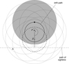 |
Fig. 1. Drift of a wide emission region (grey) around the dipole axis. Far from the profile centre (point A), the region is visible within a limited interval of drift cycle, and strong modulations appear. The extra beam (dashed) on the opposite side of the dipole axis is required to explain the jump by half of the modulation cycle. |
2. Radio pulsar beam geometry
The modulation properties of PSR B1919+21 and B1237+25 (see Figs. 3 and 2 in Proszynski & Wolszczan 1986) provide fair guidance for the beam structure. In the profile periphery, the drifting beam of Fig. 1 is visible only through a limited part of drift period, Pd, which corresponds to the grey circle passing through point A in Fig. 1. However, closer to the profile centre (thus closer to the dipole axis), this grey beam must be missing (since a peak flux is replaced with a minimum in the modulation pattern), and another beam must be located at a half modulation cycle later. Half of a modulation phase corresponds to Pd/2; therefore, the near-axis beam must be located on the other side of the dipole axis (the dashed circle in Fig. 1). We must have an outer sub-beam and an inner sub-beam, each on the opposite side of the polar tube. In fact, the polar tube is predicted to be divided into the outer and inner part by the critical magnetic field lines defined by the Goldreich-Julian charge density. This leads to the geometry shown in Fig. 2a. If the altitude scaling is ignored (∝r1/2), the grey outer arc has a radial width of 1.5θpc − 1.5θcr.
 |
Fig. 2. Basic beam pattern (a) with possible modifications. (a): fixed-altitude emission at all magnetic co-latitudes. The outer and inner circles correspond to the last open and critical B-field lines, respectively. (b): emission from the last open and critical lines within a finite altitude range. (c): arbitrary geometry of sub-beams. (d): radially extended azimuthal structure as invoked from PSR B0826−34. |
The illustrated structure presents an average beam and reflects only crucial features. For example, the partial overlap of the sub-beams in co-latitude θ, likely resulting from magnetic line curvature, is ignored; however, this aspect is not important for understanding the key modulation properties. Another beam of Fig. 2b shows the radially extended case, in which the radio emission is limited to the critical and last open field lines. The beam consists of two half-rings that result from the flaring of B-field lines. In Fig. 3 the azimuthal extent has been limited to allow for nulling in the case of near-central viewing. The beam is shown in the co-drifting frame, that is, the beam rotates around its centre (and dipole axis) at period Pd. In the case of resonant drift (nP = mPd), the beam is passed along a fixed set of viewing paths that are shown in the figure for low resonance orders. The paths keep a constant impact angle, β (angular distance from the drift or beam centre) and are marked with numbers that give their steadily increasing angle of orientation. The passage typically occurs either only from the numbered tip to the tip without the number or vice versa. To pass in both directions requires special conditions (β = 0 and, for example, Pd = n2P).
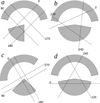 |
Fig. 3. Head-on view of a generic radio pulsar beam (grey) invoked from pulse modulation properties. Thin solid sections present the paths of sightline for low-order resonant drift (nP = mPd) and different impact angles, β′. Numbers are consecutive azimuths in beam frame. The left-side cases show the asymmetry invoked for several pulsars. |
2.1. Origin of pulsation modes and nulling
In the case of non-resonant sampling, the viewing paths may slowly rotate with respect to the beam (while keeping the fixed β ≠ 0). When the viewing path rotates through the horizontal orientation orthogonal to the beam symmetry plane (which is vertical in Fig. 3), the pulsation mode is changed. When β is small and the sub-beams do not span 180° in azimuth, a null will be observed between pulsation modes. This is where nulls are indeed often observed in pulsars (e.g., Fig. 5 in Srostlik & Rankin 2005).
For β = 0 and a uniform motion of viewing paths through the beam, only the nulling and two pulsation modes would be possible: ‘outer sub-beam–inner sub-beam’ and ‘inner–outer’. However, for β ≠ 0 at least four pulsation modes are possible: ‘outer–inner’, ‘inner–outer’, ‘outer–outer’, and ‘inner’ or ‘core’. Moreover, in the case of the resonant drift, the beam is sampled at a fixed set of paths with specific orientations. Then, the resonant set of viewing paths can define a number of profile shapes that are repeatedly observed in consecutive order. For example, in the top-right case in Fig. 3, three different pulse shapes will be observed. In the case of disturbance of the drift motion (e.g., the charge flow stop and revival), the relative phase of the viewed paths and the beam orientation can change, which can also change the pulsation mode. For peripheral viewing (β larger than the inner sub-beam radius), only the outer sub-beam can be detectable, which can lead to a nulling behaviour of a different type than for the central sightline passage.
2.2. Interpretation of PSR B1237+25
PSR B1237+25 exhibits a sequence of pulsation modes that are consistent with the not-quite-resonant rotation of the viewing path with respect to the beam in Fig. 3. In one of the modes, the components appear first at the leading side (LS) of the profile, then at the trailing side (TS), and finally in the centre. The sequence has been interpreted as a spiral motion (the S-burst in Hankins & Wright 1980). Since Pd ∼ 2.8P is close to 3P in B1237+25, the burst can be tentatively interpreted with Fig. 3d. Let the first passage correspond to the viewing path marked 120 (with the sightline moving towards the number). This produces the LS outer conal component and the inner conal component on the TS (see the top pulse in Fig. 2 of Hankins & Wright 1980). In the next pulse, the path at 240 is followed (again, towards the end with the number), producing the LS inner conal component and the TS outer conal component. In the third period the inner cone-core complex is observed along path 0. Sometimes all five components are observed together (see Fig. 2 in Hankins & Wright 1980), which suggests that the inner and outer sub-beams temporarily and partially overlap in azimuth (as on the left side in Fig. 2c). The model can explain several other effects observed in PSR B1237+25, for example the tendency for the appearance of component 1 together with 4, and of component 2 together with 5. The abnormal mode from Srostlik & Rankin appears when the viewing moments pick up the LS of the inner cone-core complex. The modes are changed when the viewing path traverses through the blank space between the inner and outer sub-beams, which can lead to the intermodal nulling when this drift phase happens to be sampled. The modes can also change with partial nulls or without nulls. The latter may happen for several reasons, the most important being the asymmetry of the inner sub-beam shown in Fig. 3a: While passing through the vertical orientation, the outer half-cone is always visible, but the sightline gains (or loses) the view of the inner beam without a null.
The conclusion is that the overall modulation properties of PSR B1237+25, along with several details, can be understood as the result of the sampling of the beam shown in Fig. 3. The spiral is not required (though two spiraling arcs could be inscribed into the grey sub-beams, sharing the basic properties of the zonal beam: imagine the thick solid arcs as having different θ at each end).
2.3. Examples of modelled pulsation modes
A simple code samples the beams of Fig. 3 at rotation angles
![Mathematical equation: $$ \begin{aligned} \Phi _{\rm cut}=(2\pi /P_{\rm d})(i_{\rm p} + W_j/360^\circ ) + \phi _{\rm ct0} \ \mathrm{[rad]} , \end{aligned} $$](/articles/aa/full_html/2021/09/aa41243-21/aa41243-21-eq1.gif) (1)
(1)
where Pd is in P, ip is the pulse number, ϕct0 (in radians) is a constant reference drift phase, and Wj (in degrees) is the vector of longitudes (of pulse width length). The viewing path (Wj, β) is then rotated by Φcut while maintaining the fixed impact angle β = β′1.5θpc. The intra-beam polar coordinates (ϕb, θb) are then calculated for each Wj, and the conditions to fall into the grey area of Fig. 3 are applied, which includes the azimuthal span of the sub-beams: Δϕout and Δϕin or, more generally, the beam limiting azimuths  ,
,  ,
,  , and
, and  . The size ratio of the radial zones is here assumed to be fixed by θcr/θpc but in general involves
  ,
,  ,
,  , and
, and  . Asymmetries and overlaps of the sub-beams are controlled by the last eight parameters.
Example code output is shown in Fig. 4. The top-right panel is for the symmetric beam of Fig. 3b, whereas the other cases are for the asymmetric beam of Fig. 3a.
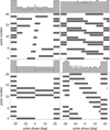 |
Fig. 4. Single pulses calculated for the beam types shown in grey at the top of Fig. 3. The figure shows several classical single pulse effects: left-right-middle modulation with core pulses (top left), jump by half of the modulation phase, with sporadic nulls in pulses 2 and 19 (top right), pulsation mode change at intermodal nulling (bottom left), and interior drift of sub-pulses flanked by fixed-longitude flux modulations (bottom right). The corresponding partial profiles are shown on top with a line and the average profiles for 2000 pulses in grey. Parameter values are (from left to right, top to bottom) Pd = 2.9, 4.2, 2.8, 1.9, β′= − 0.1, 0.1, 0, 0.4, |


The top-left case (Pd = 2.9P, β′= − 0.1) reveals the left-right-middle sequence that so misleadingly resembles the spiral in B1237+25 (Hankins & Wright 1980). We note that there is a core component despite no core being in the beam. In the top-right case (Pd = 4.2P, β′ = 0.1) the symmetric beam results in the half-phase modulation jumps, such as those observed in B1919+21. We note the sporadic single pulse nulls at pulses 2 and 19. The bottom-left case (Pd = 2.8P, β′ = 0.0) shows clear changes in pulse modes separated by intermodal nulls, such as those observed in B1237+25 (Fig. 5 in Srostlik & Rankin 2005). The bottom-right case shows a clear interior drift flanked by the fixed-longitude modulation, which is observed in several objects (e.g., B1918+19).
The pulsations have an obvious tendency to take on a quasi-conal look with several asymmetries, which are mostly related to the sub-beam being located on each side of the profile. Interestingly, pulses from an apparently inner cone are sometimes visible in several patterns, despite only one half-cone and a birthday-cake-like wedge being in the beam. They arise from cutting the corners of the sub-beams. The core component appears in many simulations even without any brightening at the beam centre and results from cutting through the central tip of the inner sub-beam.
To obtain the main types of behaviour shown in Fig. 4, in particular the nulling separating core-dominated and cone-dominated pulsation modes, the beam must be asymmetric (Fig. 3a). Then, over some limiting azimuths the outer sub-beam may be sampled without the inner sub-beam visible, with mode transition occurring either at nulls or without nulls (bottom-left case in Fig. 4). Though not shown, the model also produces the antisymmetric profiles with only one side bright. The zonal structure of the beam implies correlations between a main pulse (MP) and an inter-pulse (IP), as well as anti-correlations (Weltevrede et al. 2012).
It is found that several classical types of single pulse behaviour, reported in a multitude of observations, can be interpreted with the sector (zonal) beam of Fig. 3.
To properly model the average profiles, a more realistic emissivity profile (non-uniform) must still be implemented. However, calculations made so far make it clear that the question of whether the average profile is brightest at the edges or at the centre clearly depends on the ratio Rϕ = Δϕout/Δϕin and not only on the impact parameter. The average profiles shown in grey in Fig. 4 correspond to the uniform and equal emissivity within the sub-beam zones. If the drift is not resonant, the strength ratio of central to peripheral components roughly corresponds to the ratio of the azimuthal extent of the sub-beams, Rϕ = Δϕin/Δϕout. The top-right case in Fig. 4 has a boxy shape since Rϕ = 1, whereas in the other cases Rϕ = 0.5, hence, the average profiles have a bright periphery and correspond to a double type (or perhaps a blended multiple with bright edges). Beyond the proposed model, the diversity of average profiles may furthermore be increased by the dependence of magnetospheric current flow on dipole tilt and by polarization-mode-sensitive effects (absorption, scattering, refraction).
The fractional azimuthal extent also affects the statistics of nulling. In the case of non-resonant drift and β = 0, the fraction of nulls corresponds to the fraction of azimuths that are radio quiet on both sides of the beam (at ϕ and ϕ + π). For β ≠ 0 the null fraction is no longer trivial to estimate because it depends on both the azimuthal and radial (Δθ) extent of the sub-beams. For example, when the beam becomes narrow in azimuth (Δϕ ≪ Δθ), it is β and Δθ that determine the null fraction.
Furthermore, the model implies two types of nulling, central and peripheral. The second type appears when our line of sight is just grazing the beam, with  . In this case the nulling fraction essentially corresponds to (2π − Δϕout)/2π. A sample of nulling pulsars may thus contain objects that null in either way (central or peripheral).
If the drift period is resonant, the null statistics and average profiles are affected by the ratio Pd/P. The null fraction and the profile shapes then depend on the absolute phase of drift with respect to star spin phase. Depending on the drift stability, both periodic and non-periodic nulls are possible (Basu et al. 2020).
The proposed geometry implies that, generally, the null fraction increases when the azimuthal extent of the sub-beams decreases. Space-charge limited flow models (discussed in the next section) predict that accelerating voltage decreases with distance from the main meridian (Ω − μ plane). In older pulsars (closer to the death line) the pair production may thus be possible only close to the Ω − μ plane. In such objects the sub-beams may then have a smaller azimuthal extent. This is in line with the finding, in Wang et al. (2007), that older pulsars tend to have larger null fractions; that paper also concludes that ‘nulling and mode changing are different manifestations of the same phenomenon’, which is consistent with the model proposed here.
It is unclear if the model applies to the extremely long nulling observed in state switching pulsars (Kramer et al. 2006; Young et al. 2015; Stairs et al. 2019) because this requires special conditions: For the long nulls, the drift must be essentially resonant or extremely slow. Moreover, the spin down would have to depend on the drift phase.
2.4. Fine beam structure: Lesson from B0826−34
The observation of several sub-pulses in a single pulse implies that, at least for some objects, the sub-beams must be azimuthally structured (if the time modulation of the sub-beams is excluded). PSR B0826−34 offers insight here because its beam is nearly parallel to the rotation axis and the pulsar is viewed at a small viewing angle (Esamdin et al. 2005; Gupta et al. 2004). The low-flux minima separating the MP from the IP in this object have been interpreted as evidence for two nested carousels separated in co-latitude (Fig. 10 in Esamdin et al. 2005). However, according to the generic beam of Fig. 3, the IP must correspond to the inner-sub-beam wedge and the MP to the outer half-cone sub-beam. The observed MP and IP are thus separated by the blank space that separates the sub-beams in magnetic azimuth. To account for the observed sub-pulses, the brightest parts of the beam extend radially from the dipole axis, as shown in Fig. 2d. There is just the radial (spoke-like) structure with the break in the azimuth (instead of two nested cones with the break in co-latitude). The data on B0826−34 (Fig. 1 in Esamdin et al. 2005) also imply that the inner sub-beam has spectral properties that are quite different from those of the outer cone. This is another factor that affects the average profile shape. The back-and-forth motion of components suggests the sub-beams may wiggle back and forth instead of following the monotonic E × B rotation.
3. Structure of particle flow
Assuming that charges within the polar tube are generally capable of emitting detectable radio emission, the blank parts of the invoked beam (Fig. 3) can be interpreted as regions with particles flowing away from the observer. This leads to the particle flow pattern shown in Fig. 5.
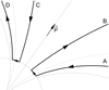 |
Fig. 5. Particle flow pattern suggested by the beam in Fig. 3. A reversed flow of emitting particles (with all arrows reversed) is also possible. The last open lines are dashed, the critical lines are dotted, and μ is the dipole magnetic moment. |
The inward flow in regions A and C turns numerous exotic ideas into reasonable possibilities. If downward flow A is radiating, the radiation may be obscured at flow B, it can be scattered there, or it can be mirror-style reflected. It may also pass through to the other side, forming the off-pulse quasi-isotropic radiation. Extremely wide pulse components with strange absorption features (not only double notches) have been observed, for example in PSR B0950+08 and B1929+10 (Rankin & Rathnasree 1997; McLaughlin & Rankin 2004), although not in other pulsars (e.g., Kramer et al. 2002). The asymmetry in Fig. 5 seems consistent with the non-universal character of this phenomenon.
When different magnetic azimuths are considered, the emission from flow A is always directed towards the near-axial region, which leads to interesting ray focusing geometry. Moreover, it is now possible to assume that the radio signal is produced at high altitudes in a weaker magnetic field but is emitted inwards, where it is reflected or scattered outwardly. Similar bidirectional effects are expected for flow CD; however, since flow C is more vertical, its radiation is more likely to be reflected outwards by the star surface or a central plasma region.
The loops of flow in Fig. 5 (such as AB between the periphery and centre of the polar tube) are generally consistent with expectations (Fig. 3 in Mestel & Shibata 1994). However, the antisymmetry around μ is yet to be understood. The local excess of charge density depends on whether local B-field lines bend towards the closest rotational pole or towards the equator. Therefore, the accelerating electric field E∥ is opposite in two semicircles of a polar cap (Arons & Scharlemann 1979; Mestel & Shibata 1994). When the semicircles are superposed on a ring in a polar tube, the pattern of Fig. 2a can be expected. While referring to the semicircular acceleration region, Beskin (2010, p. 109) states that ‘accordingly, the radiation emissivity pattern should also have the form of a semicircle. However, this conclusion contradicts the observational data’. As shown above, the semicircle (and a half-ring) can be invoked from the checkerboard-like modulation pattern. Still, the semicircle of, say, poleward-bending B-field lines does not drift around the dipole axis. On the other hand, if the lateral drift is attributed to the outflowing plasma (rather than to the pattern of E∥), it may be difficult to maintain the drifting sub-beams because the relativistic particles escape the magnetosphere in about 1/6 of P. Finally, the ring of critical field lines is expected for small or mild dipole inclinations and depends on the outer gap activity. Instead, it is possible that the outer half-ring of the invoked beam corresponds to the return current sheet (see Fig. 1 by X. Bai in Timokhin & Arons 2013).
4. Conclusions
The radio pulsar beam is sector-structured both in azimuth and magnetic co-latitude and is indeed E × B-drifting around the dipole axis. The sub-beam zones are essentially antisymmetric, as implied by the checkerboard-like modulation patterns observed in PSR B1919+21 and B1237+25. The long timescales of pulse moding and nulling result from the near resonance of Pd and P, which causes a very slow rotation of viewing path through the beam.
The established geometry produces pulsations that bear an obvious and striking resemblance to the single pulse observations, explain several types of typically observed behaviour, and allow for a much larger diversity of effects than the axially symmetric carousel. Moreover, the zonal beam is in line with the general structure of the magnetospheric charge density distribution.
Although multiple questions about the beam details remain open, the beam is capable of explanations that are beyond the reach of the standard carousel model or the surface oscillation model, making these models obsolete. However, the results support the cone size origin proposed by Wright (2003). It is clear that it becomes possible to apply the proposed beam to several observed effects and objects, which should allow the beam geometry and behaviour to be better constrained.
Acknowledgments
This work was supported by the grant 2017/25/B/ST9/00385 of the National Science Centre, Poland.
References
- Arons, J., & Scharlemann, E. T. 1979, ApJ, 231, 854 [NASA ADS] [CrossRef] [Google Scholar]
- Basu, R., Mitra, D., & Melikidze, G. I. 2020, ApJ, 889, 133 [CrossRef] [Google Scholar]
- Beskin, V. S. 2010, MHD Flows in Compact Astrophysical Objects (Berlin, Heidelberg: Springer Verlag) [Google Scholar]
- Clemens, J. C., & Rosen, R. 2008, ApJ, 680, 664 [NASA ADS] [CrossRef] [Google Scholar]
- Dai, S., Hobbs, G., Manchester, R. N., et al. 2015, MNRAS, 449, 3223 [NASA ADS] [CrossRef] [Google Scholar]
- Edwards, R. T., Stappers, B. W., & van Leeuwen, A. G. J. 2003, A&A, 402, 321 [NASA ADS] [CrossRef] [EDP Sciences] [Google Scholar]
- Esamdin, A., Lyne, A. G., Graham-Smith, F., et al. 2005, MNRAS, 356, 59 [NASA ADS] [CrossRef] [Google Scholar]
- Gupta, Y., Gil, J., Kijak, J., & Sendyk, M. 2004, A&A, 426, 229 [NASA ADS] [CrossRef] [EDP Sciences] [Google Scholar]
- Hankins, T. H., & Wright, G. A. E. 1980, Nature, 288, 681 [CrossRef] [Google Scholar]
- Kirk, J. G., Skjæraasen, O., & Gallant, Y. A. 2002, A&A, 388, L29 [NASA ADS] [CrossRef] [EDP Sciences] [Google Scholar]
- Kramer, M., Johnston, S., & van Straten, W. 2002, MNRAS, 334, 523 [NASA ADS] [CrossRef] [Google Scholar]
- Kramer, M., Lyne, A. G., O’Brien, J. T., Jordan, C. A., & Lorimer, D. R. 2006, Science, 312, 549 [NASA ADS] [CrossRef] [PubMed] [Google Scholar]
- Maan, Y. 2019, ApJ, 870, 110 [CrossRef] [Google Scholar]
- McLaughlin, M. A., & Rankin, J. M. 2004, MNRAS, 351, 808 [NASA ADS] [CrossRef] [Google Scholar]
- McSweeney, S. J., Bhat, N. D. R., Wright, G., Tremblay, S. E., & Kudale, S. 2019, ApJ, 883, 28 [NASA ADS] [CrossRef] [Google Scholar]
- Mestel, L., & Shibata, S. 1994, MNRAS, 271, 621 [NASA ADS] [Google Scholar]
- Proszynski, M., & Wolszczan, A. 1986, ApJ, 307, 540 [NASA ADS] [CrossRef] [Google Scholar]
- Rankin, J. M. 1983, ApJ, 274, 333 [NASA ADS] [CrossRef] [Google Scholar]
- Rankin, J. M. 1990, ApJ, 352, 247 [NASA ADS] [CrossRef] [Google Scholar]
- Rankin, J. M. 1993, ApJ, 405, 285 [NASA ADS] [CrossRef] [Google Scholar]
- Rankin, J. M., & Rathnasree, N. 1997, JApA, 18, 91 [NASA ADS] [Google Scholar]
- Rankin, J. M., Wright, G. A. E., & Brown, A. M. 2013, MNRAS, 433, 445 [NASA ADS] [CrossRef] [Google Scholar]
- Ruderman, M. A., & Sutherland, P. G. 1975, ApJ, 196, 51 [NASA ADS] [CrossRef] [EDP Sciences] [Google Scholar]
- Srostlik, Z., & Rankin, J. M. 2005, MNRAS, 362, 1121 [NASA ADS] [CrossRef] [Google Scholar]
- Stairs, I. H., Thorsett, S. E., & Camilo, F. 1999, ApJS, 123, 627 [NASA ADS] [CrossRef] [Google Scholar]
- Stairs, I. H., Lyne, A. G., Kramer, M., et al. 2019, MNRAS, 485, 3230 [NASA ADS] [CrossRef] [Google Scholar]
- Timokhin, A. N., & Arons, J. 2013, MNRAS, 429, 20 [NASA ADS] [CrossRef] [Google Scholar]
- van Leeuwen, A. G. J., Stappers, B. W., Ramachandran, R., & Rankin, J. M. 2003, A&A, 399, 223 [NASA ADS] [CrossRef] [EDP Sciences] [Google Scholar]
- Wang, N., Manchester, R. N., & Johnston, S. 2007, MNRAS, 377, 1383 [NASA ADS] [CrossRef] [Google Scholar]
- Weltevrede, P. 2016, A&A, 590, A109 [NASA ADS] [CrossRef] [EDP Sciences] [Google Scholar]
- Weltevrede, P., Wright, G., & Johnston, S. 2012, MNRAS, 424, 843 [NASA ADS] [CrossRef] [Google Scholar]
- Wright, G. A. E. 2003, MNRAS, 344, 1041 [NASA ADS] [CrossRef] [Google Scholar]
- Young, N. J., Weltevrede, P., Stappers, B. W., Lyne, A. G., & Kramer, M. 2015, MNRAS, 449, 1495 [CrossRef] [Google Scholar]
All Figures
|
Fig. 1. Drift of a wide emission region (grey) around the dipole axis. Far from the profile centre (point A), the region is visible within a limited interval of drift cycle, and strong modulations appear. The extra beam (dashed) on the opposite side of the dipole axis is required to explain the jump by half of the modulation cycle. |
| In the text | |
|
Fig. 2. Basic beam pattern (a) with possible modifications. (a): fixed-altitude emission at all magnetic co-latitudes. The outer and inner circles correspond to the last open and critical B-field lines, respectively. (b): emission from the last open and critical lines within a finite altitude range. (c): arbitrary geometry of sub-beams. (d): radially extended azimuthal structure as invoked from PSR B0826−34. |
| In the text | |
|
Fig. 3. Head-on view of a generic radio pulsar beam (grey) invoked from pulse modulation properties. Thin solid sections present the paths of sightline for low-order resonant drift (nP = mPd) and different impact angles, β′. Numbers are consecutive azimuths in beam frame. The left-side cases show the asymmetry invoked for several pulsars. |
| In the text | |
|
Fig. 4. Single pulses calculated for the beam types shown in grey at the top of Fig. 3. The figure shows several classical single pulse effects: left-right-middle modulation with core pulses (top left), jump by half of the modulation phase, with sporadic nulls in pulses 2 and 19 (top right), pulsation mode change at intermodal nulling (bottom left), and interior drift of sub-pulses flanked by fixed-longitude flux modulations (bottom right). The corresponding partial profiles are shown on top with a line and the average profiles for 2000 pulses in grey. Parameter values are (from left to right, top to bottom) Pd = 2.9, 4.2, 2.8, 1.9, β′= − 0.1, 0.1, 0, 0.4, |
| In the text | |
|
Fig. 5. Particle flow pattern suggested by the beam in Fig. 3. A reversed flow of emitting particles (with all arrows reversed) is also possible. The last open lines are dashed, the critical lines are dotted, and μ is the dipole magnetic moment. |
| In the text | |
Current usage metrics show cumulative count of Article Views (full-text article views including HTML views, PDF and ePub downloads, according to the available data) and Abstracts Views on Vision4Press platform.
Data correspond to usage on the plateform after 2015. The current usage metrics is available 48-96 hours after online publication and is updated daily on week days.
Initial download of the metrics may take a while.