© ESO 2022

1. Introduction

Thanks to recent progress in high-performance computing, radiation hydrodynamics (RHD) simulations are now popular in many research fields in astrophysics. Accordingly, numerical schemes for RHD simulations have been developed. However, it is also crucial to use appropriate opacities in order to obtain correct solutions of RHD equations, which is the focus of this study. To save computational time in RHD simulations, it is fairly common to solve a frequency-averaged radiative transfer equation with the local thermodynamic equilibrium (LTE) assumption. In this case, Rosseland and Planck mean opacities as functions of temperature and pressure are required to perform RHD simulations (e.g., Hirose et al. 2014).

Although the methods for calculating gas opacities have been established, significant effort is required to calculate them in practice. For example, one has to gather data pertaining to relevant opacity sources scattered throughout the literature or on the web and develop complicated interfaces capable of reading various types of data. Moreover, it is computationally intensive to calculate line opacities from very large line lists such as those provided by Exomol¹ (Tennyson & Yurchenko 2012). Therefore, researchers tend to use publicly available opacity tables. In the literature, there are a number of papers that provide opacity tables (Cox & Stewart 1970a,b; Alexander 1975; Alexander et al. 1983; Sharp 1992; Alexander & Ferguson 1994; Bell & Lin 1994; Pollack et al. 1994; Henning & Stognienko 1996; Helling et al. 2000; Semenov et al. 2003; Ferguson et al. 2005; Freedman et al. 2008; Helling & Lucas 2009; Malygin et al. 2014), including OPAL Project² (Rogers & Iglesias 1992) and Opacity Project³ (Seaton et al. 1992).

As summarized in Table A.1 in Semenov et al. (2003), the various opacity tables differ depending on the research purpose and thus differ in composition, opacity sources, ranges of temperature and pressure, and outputs. Consequently, one cannot always obtain an opacity table that meets one’s research purpose. One can create a hybrid table that covers larger ranges by combining different tables (e.g., Fig. 2 in Hirose et al. 2014); however, it is not guaranteed that the tables will share the same boundary values. As pointed out by Malygin et al. (2014), disagreements in opacity values between different tables could be caused not by only different assumptions being applied but also because of the use of different sampling points. This makes comparison of different opacity tables difficult unless table codes are publicly available. Another issue is that not all public tables are updated regularly.

For these reasons, we decided to develop a public code, named OPTAB, that can be used to generate opacity tables using opacity sources and sampling points chosen by the user. In the first version of the code, we consider only gas opacities, whose physics are well understood. Our code outputs Rosseland, Planck, and two-temperature Planck mean opacities, as well as the monochromatic opacity. The two-temperature Planck mean opacity (Eq. (28)) is needed when one considers the case in which the radiation and gas temperatures differ, such as an accretion disk irradiated by the central star (e.g., Hirose & Shi 2019). In the literature, the public code DFSYNTHE (Castelli 2005) can be used to generate opacity tables (Malygin et al. 2014). Additionally, OPAL⁴ (Rogers & Iglesias 1992) and Semenov et al. (2003)⁵ provide public codes for generating opacity tables. In contrast to these codes, our code is developed for modern high-performance computing – it is written in Fortran 90 using Message Passing Interface (MPI) and Hierarchical Data Format, Version 5 (HDF5)⁶ – and addresses both readability and portability. Furthermore, our code is available at GitHub⁷ and allows for continuous updates through contributions by users.

The goal of this code is not to provide complete opacity tables for a specific purpose, but to provide a platform on which users can generate opacity tables for their own purposes. Therefore, while opacity sources initially implemented in our code are basic ones, the code is written so that a user can easily modify, change, or add opacity sources.

We note that OPTAB does not solve the chemical equilibrium (CE) condition to obtain equilibrium abundances of species that are needed for calculating opacities. We assume that the user has obtained this solution using an external program. Recently, public CE solvers for astrophysics, including FASTCHEM (Stock et al. 2018) and TEA (Blecic et al. 2016), have been made available.

In Sect. 2, the structure of the code and the opacity sources implemented in our code are described. In Sect. 3, the details of the opacity calculations in our code are given. In Sect. 4, a method to reduce the computational effort in line opacity calculations is described. In Sect. 5, the results of validation tests to evaluate the performance of our code are presented. Finally, future aspects are discussed in Sect. 6.

2. Code description

OPTAB is written in Fortran 90 using the MPI library for parallel computing as well as the HDF5 library for flexible and efficient parallel Input/Output (I/O) of very large atomic or molecular line lists.

In Table 1, we list the opacity sources implemented in the first version of OPTAB. All sources are publicly available, and the choice of sources is based on the PHOENIX code (Hauschildt & Baron 1999; Allard & Hauschildt 1995)⁸. Because each subroutine calculating each opacity is modularized, the user can easily modify the code to change or add opacity sources. To calculate opacities, in addition to the opacity sources, some supplementary data providing atomic properties are needed, which are obtained from the National Institute of Standards and Technology (NIST) Atomic Spectra Database (ASD) levels form⁹ (Kramida et al. 2020) and NIST Atomic Weights and Isotopic Compositions with Relative Atomic Masses (AWIC)¹⁰ (Meija et al. 2016; Berglund & Wieser 2011).

As shown in Table 1, OPTAB currently accepts the Kurucz line lists¹¹ for atomic lines, and the HITRAN¹² (Gordon et al. 2017) and Exomol line lists for molecular lines. Because these line lists are extremely large and are repeatedly accessed in the code, they are converted to HDF5 files from their original ASCII files beforehand. In addition, HITRAN collision-induced absorption (CIA) data and the supplementary data for atomic properties taken from the NIST ASD/AWIC are converted and stored in an HDF5 file, respectively. The details of these conversions are described in Appendix A.

Figure 1 shows the flowchart for OPTAB. First, the code reads parameters that determine the opacity sources to be considered, the wave number grid ${\stackrel{\sim }{\nu }}_k$ [cm⁻¹] (k is the grid index), and the line profile evaluation described in Sect. 4. Then, it reads CE abundances based on which the opacities are computed, which are prepared by the user for some pairs of temperature and pressure (i.e., “layers”). The equilibrium abundances needs to be stored in a specified HDF5 format; the OPTAB package provides codes for storing the outputs of FASTCHEM and TEA in the HDF5 format.

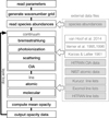Fig. 1. Flowchart of OPTAB. The external files in the gray boxes are in the HDF5 format, which have been converted from their original ASCII files (Appendix A).

After reading the above data, the code computes the continuum opacities, line opacities, and the mean opacities, and repeats the computations for each layer. Here, opacity sources of small size are coded inline, while those of large size are read from external files. MPI parallelization is performed for the layer loop (Sect. 5.3). As the final step of the layer loop, the absorption and scattering coefficients together with the mean opacities for each layer are written into a single HDF5 file.

3. Opacity calculations

While we use the wavenumber $\stackrel{\sim }{\nu }$ for the computational grid in OPTAB, we also use the frequency $\nu =c\stackrel{\sim }{\nu }$, photon energy $E=hc\stackrel{\sim }{\nu }$, or wavelength $\lambda =1/\stackrel{\sim }{\nu }$ in the following sections, depending on the context. Here, c and h are the speed of light and the Planck constant, respectively.

3.1. Notes on partition functions

The opacity calculation for LTE gas uses the fact that the level population obeys the Maxwell-Boltzmann distribution, where the number density of a species in energy level l at temperature T and pressure P is written as

$$\begin{array}{c}\hfill N_l(T,P)=N(T,P){\displaystyle \frac{g_l{\mathrm{e}}^{-\frac{E_l-E_1}{k_{\mathrm{B}}T}}}{Q(T)}}.\end{array}$$(1)

Here, Q(T) is the internal partition function defined as

$$\begin{array}{c}\hfill Q(T)\equiv {\displaystyle \sum _l{g}_l{\mathrm{e}}^{-\frac{E_l-E_1}{k_{\mathrm{B}}T}},}\end{array}$$(2)

g_l and E_l are the statistical weight and energy of the level l, respectively (E₁ is the energy of the ground state), and k_B is the Boltzmann constant.

The total number density N(T, P) = ∑_lN_l(T, P) in Eq. (1) for each species is determined by a CE calculation, where Q(T) also plays an important role. This is because the chemical potential μ(T, P) [J mol⁻¹] used in a CE calculation is uniquely related to Q(T) as

$$\begin{array}{c}\hfill \mu (T,P)-N_{\mathrm{A}}{E}_1=RTln\left({\displaystyle \frac{P}{k_{\mathrm{B}}T}}{\left({\displaystyle \frac{h^2}{2\pi m{k}_{\mathrm{B}}T}}\right)}^{\frac{3}{2}}{\displaystyle \frac{1}{Q(T)}}\right),\end{array}$$(3)

where N_A is the Avogadro constant [mol⁻¹], R is the gas constant [J K⁻¹ mol⁻¹], and m is the mass of the atom or molecule (Eq. (24.50) in McQuarrie & Simon 1997). Therefore, for the LTE opacity to be consistent with the CE, the same partition function should be used. For more details, we refer the readers to Appendix C.

In practice, this cannot be done for the following reasons: i) In a CE calculation, μ is usually computed from thermochemical databases based on experiments such as NIST-JANAF (Chase 1998) or NASA Chemical Equilibrium with Applications (CEA) (Mcbride & Gordon 1992). However, because such thermochemical databases do not consider isotoplogues, they cannot be used to calculate Q(T) (by means of Eq. (C.4)) for the LTE opacity calculations, in which isotopologues are considered. ii) On the other hand, the number of species for which Q(T) is provided along with the line lists is not sufficient for performing a CE calculation. For example, the number of molecular species in the HITRAN line lists is 55, whereas that used in a CE solver FASTCHEM is 436 (Table 2 in Stock et al. 2018).

Because of reasons (i) and (ii), we have to admit that in practice different partition functions may be used between the CE calculation and the LTE opacity calculations. In our code, for Kurucz atomic lines, we use the Kurucz level data gf????(z).gam¹³ to calculate Q(T) from the definition (Eq. (2)). We note that the Kurucz level data are not available for some species, for which we use the NIST ASD levels instead. For molecular lines, we employ tabulated partition functions provided with the line lists.

Hereafter, we omit the dependence of number densities N on temperature T and pressure P for brevity. Accordingly, we omit the dependence of absorption coefficients α [cm⁻¹] on P.

3.2. Bremsstrahlung

The absorption coefficient of the bremsstrahlung of an atomic ion of charge Ze (where Z ≥ 1 is the charge number and e is the elementary charge) is written as (e.g., Rybicki & Lightman 2008)

$$\begin{array}{c}\hfill {\displaystyle \frac{{\alpha }_{\mathrm{bre}}(\nu ;T)}{N_{\mathrm{e}}{N}_{\mathrm{ion}}}}=\left({\displaystyle \frac{4}{3}}\sqrt{{\displaystyle \frac{2\pi m_{\mathrm{e}}}{3}}}{\displaystyle \frac{e^6}{m_{\mathrm{e}}^{2}ch}}\right){\displaystyle \frac{1-{\mathrm{e}}^{-\frac{h\nu }{k_{\mathrm{B}}T}}}{\sqrt{k_{\mathrm{B}}T}{\nu }^3}}{Z}^2{\overline{g}}_{\mathrm{ff}}({\gamma }^2,u).\end{array}$$(4)

Here, the thermally averaged Gaunt factor, ${\overline{g}}_{\mathrm{ff}}$, is a function of the scaled quantities γ² ≡ Z²Ry/k_BT and u ≡ hν/k_BT, and N_e, N_ion, and m_e are the number densities of free electrons and ions, and the electron mass, respectively. Ry is an energy unit, the Rydberg, which is approximately 13.6 eV. Our code employs a numerical table for ${\overline{g}}_{\mathrm{ff}}({\gamma }^2,u)$ provided by Hoof et al. (2014) to compute Eq. (4) for elements ranging from hydrogen (H) to zinc (Zn). Then, the total coefficient is obtained by summing up the coefficients of H⁺, He⁺, He²⁺, …, and Zn³⁰⁺.

In addition, we have implemented the bremsstrahlung absorption of H⁻ and ${\text{H}}_2^{\text{−}}$ based on John (1988) and John (1978), respectively. In the former, the absorption coefficient per electron pressure (P_e) per number density of H (N_H) [cm² dyne⁻¹] is given as a function of λ and T. In the latter, the absorption coefficient per P_e per N_H2 is given as a function of $\stackrel{\sim }{\nu }$ and T.

3.3. Photoionization

A general expression for the photoionization absorption coefficient is

$$\begin{array}{c}\hfill {\alpha }_{\mathrm{pho}}(\nu ;T)=(1-{\mathrm{e}}^{-\frac{h\nu }{k_{\mathrm{B}}T}}){\displaystyle \sum _l{\sigma }_l{N}_l,}\end{array}$$(5)

which is rewritten using Eq. (1) as

$$\begin{array}{c}\hfill {\displaystyle \frac{{\alpha }_{\mathrm{pho}}(\nu ;T)}{N}}=(1-{\mathrm{e}}^{-\frac{h\nu }{k_{\mathrm{B}}T}}){\displaystyle \frac{1}{Q(T)}}{\displaystyle \sum _l{\sigma }_l{g}_l{\mathrm{e}}^{-\frac{E_l}{k_{\mathrm{B}}T}},}\end{array}$$(6)

where σ_l is the photoionization cross-section of energy level l, and (1 − e^−hν/k_BT) is a correction factor for the induced absorption.

For atoms and their positive ions, the last factor in Eq. (6) (a summation on the energy levels) is expressed in our code as

$$\begin{array}{cc}& {\displaystyle \sum _l{\sigma }_l{g}_l{\mathrm{e}}^{-\frac{E_l}{k_{\mathrm{B}}T}}={\sigma }_1{g}_1+\sum _{l\ge 2}{\sigma }_l{g}_l{\mathrm{e}}^{-\frac{E_l}{k_{\mathrm{B}}T}},}\hfill \end{array}$$(7)

$$\begin{array}{cc}\hfill & {\sigma }_1\equiv \{\begin{array}{cc}{\sigma }^{(\mathrm{v}96)}(E)\hfill & E\le E_{\max }\hfill \\ {\sum }_{\mathit{nm}}{\sigma }_{\mathit{nm}}^{(\mathrm{v}95)}(E)\hfill & E>E_{\max }\hfill \end{array},\hfill \end{array}$$(8)

where n and m are the principal quantum number of the shell and the subshell orbital quantum number, respectively.

Equation (8) indicates that we employ a hybrid of Verner & Yakovlev (1995) and Verner et al. (1996) (${\sigma }_{\mathit{nl}}^{(\mathrm{v}95)}$ and σ^(v96), respectively) for photoionization originating from the ground level (l = 1) depending on E_max, which is a parameter given in Verner et al. (1996) and is specific to the species. Verner & Yakovlev (1995) proposed a fitting formula to the partial photoionization cross-sections based on Hartree-Dirac-Slater calculations for the ground state shells (of elements from H to Zn). Verner et al. (1996) presented a set of analytic fits to the photoionization cross-sections (of elements from H to Si, and for S, Ar, Ca, and Fe) calculated by the Opacity Project (OP), which are more accurate at low energies. In Fig. 2, the brown curve shows how the above hybrid photoionization cross-section is applied to Mg atoms, where E_max = 54.90 eV, or $\stackrel{\sim }{\nu }=4.428\times {10}^5$ cm⁻¹.

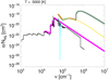Fig. 2. Magnesium photoionization absorption coefficients per Mg atom [cm2] at 5000 K. The brown curve indicates the photoionization from the ground level, and is a hybrid of Verner et al. (1996) (outer-subshell contributions; yellow) and Verner & Yakovlev (1995) (inner-subshell contributions; cyan). Both the magenta and black thin curves indicate the photoionization from excited levels; the former is based on the Mathisen (1984) compilation, whereas the latter is based on TOPbase.

As for photoionization cross-sections from excited states (l ≥ 2), OPTAB provides two options: cross-sections compiled by Mathisen (1984) and cross-sections available at the Opacity Project online atomic database, TOPbase (Cunto & Mendoza 1992). Both databases provide a set of {σ_l,g_l,E_l} for selected photoionization channels of selected species that can be used in Eq. (6). TOPbase is generally more comprehensive and more complete than the Mathisen’s compilation¹⁴. In Fig. 2, we compare the photoionization cross-sections from excited states between the Mathisen’s compilation (magenta; Vernazza et al. 1976, 1981; Thompson et al. 1974; Bradley et al. 1976) and TOPbase (thin black). We observe that more detailed structures are resolved in the TOPbase photoionization cross-sections; however, they require higher computational costs.

For H and He⁺ (hydrogenic atoms and ions), the photoionization cross-section is written in terms of Kramers’ semi-classical formula as (e.g., Carson et al. 1968)¹⁵

$$\begin{array}{c}\hfill {\sigma }_n(\nu )\equiv \left[{\displaystyle \frac{64{\pi }^4}{3\sqrt{3}}}\left({\displaystyle \frac{m_{\mathrm{e}}{e}^{10}}{c{h}^6}}\right)\left({\displaystyle \frac{Z^4}{n^5}}\right){\displaystyle \frac{1}{{\nu }^3}}\right]g({\displaystyle \frac{h\nu }{Z^2\mathrm{Ry}}},n),\end{array}$$(9)

where n is the principal quantum number. For the Gaunt factor g(hν/Z²Ry, n), fitting formulae by Chapman (1969, 1970) for the tables given in Karzas & Latter (1961) are recommended in Mathisen (1984). However, we use the original tables in our code instead because we found the fitting formulae diverge in some cases.

In addition to the above, we have implemented photoionization absorption for H⁻ and H₂. For the former and latter, we employ the cross-section formulas given in Ohmura & Ohmura (1960) and Yan et al. (2001), respectively.

3.4. Line absorption

The line absorption coefficient for the transition from state l to state u is expressed as

$$\begin{array}{c}\hfill {\alpha }_{\mathrm{line}}(\stackrel{\sim }{\nu };T)=N_l\left({\displaystyle \frac{\pi e^2}{m_{\mathrm{e}}c}}\right)f_{\mathit{lu}}{\displaystyle \frac{{\varphi }_{\mathit{ul}}(\stackrel{\sim }{\nu })}{c}}(1-{\mathrm{e}}^{-c_2\stackrel{\sim }{\nu }/T}),\end{array}$$(10)

where c₂ ≡ hc/k_B, ${\varphi }_{\mathit{ul}}(\stackrel{\sim }{\nu })$ [cm] is the line profile in terms of the wavenumber $\stackrel{\sim }{\nu }$, and f_lu is the oscillator strength from state l to state u¹⁶. Because we consider LTE, the number density at state l of the species being considered can be written as (cf. Eq. (1))

$$\begin{array}{c}\hfill N_l=x^{(\mathrm{iso})}N{\displaystyle \frac{g_l{\mathrm{e}}^{-c_2{\stackrel{\sim }{E}}_l/T}}{Q(T)}},\end{array}$$(11)

where N is the total number density of the species, and ${\stackrel{\sim }{E}}_l\equiv E_l/hc$ is the level energy in terms of the wavenumber. We have introduced the isotope or isotopologue fraction x^(iso) (cf. Appendix A) because the line transitions are different between different isotope or isotoplogues. Then the absorption coefficient is written as

$$\begin{array}{cc}& {\displaystyle \frac{{\alpha }_{\mathrm{line}}(\stackrel{\sim }{\nu };T)}{N}}=x^{(\mathrm{iso})}{S}_{\mathit{lu}}{\varphi }_{\mathit{ul}}(\stackrel{\sim }{\nu })(1-{\mathrm{e}}^{-c_2\stackrel{\sim }{\nu }/T}),\hfill \end{array}$$(12)

$$\begin{array}{cc}\hfill & S_{\mathit{lu}}\equiv \left({\displaystyle \frac{\pi e^2}{m_{\mathrm{e}}{c}^2}}\right)\left(g_l{f}_{\mathit{lu}}\right){\displaystyle \frac{{\mathrm{e}}^{-c_2{\stackrel{\sim }{E}}_l/T}}{Q(T)}},\hfill \end{array}$$(13)

where S_lu [cm] is the line intensity, and the factor (g_lf_lu) is called the g-f value.

3.5. Line profile evaluation

In our code, we generally apply the Voigt profile, a convolution of the Gaussian and Lorentzian profiles, for the line profile ${\varphi }_{\mathit{ul}}(\stackrel{\sim }{\nu })$:

$$\begin{array}{cc}& {\varphi }_{\mathit{ul}}(\stackrel{\sim }{\nu })={\displaystyle {\int }_{-\infty }^{\infty }\left\{{\displaystyle \frac{1}{\sqrt{\pi }{\sigma }_{\mathrm{G}}}}{\mathrm{e}}^{-{(({\stackrel{\sim }{\nu }}^{\prime }-{\stackrel{\sim }{\nu }}_{\mathit{ul}})/{\sigma }_{\mathrm{G}})}^2}\right\}\left\{{\displaystyle \frac{1}{\pi }}{\displaystyle \frac{\gamma }{{(\stackrel{\sim }{\nu }-{\stackrel{\sim }{\nu }}^{\prime })}^2+{\gamma }^2}}\right\}\mathrm{d}{\stackrel{\sim }{\nu }}^{\prime }}\hfill \\ \hfill & ={\displaystyle \frac{1}{\sqrt{\pi }{\sigma }_{\mathrm{G}}}}K(x,y).\hfill \end{array}$$(14)

Here, K(x, y) is the Voigt function defined as

$$\begin{array}{cc}& K(x,y)\equiv {\displaystyle \frac{y}{\pi }}{\displaystyle {\int }_{-\infty }^{\infty }{\displaystyle \frac{{\mathrm{e}}^{-t^2}}{{(x-t)}^2+y^2}}\mathrm{d}t,}\hfill \end{array}$$(15)

$$\begin{array}{cc}\hfill & x\equiv {\displaystyle \frac{\stackrel{\sim }{\nu }-{\stackrel{\sim }{\nu }}_{\mathit{ul}}}{{\sigma }_{\mathrm{G}}}},\hfill \end{array}$$(16)

$$\begin{array}{cc}\hfill & y\equiv {\displaystyle \frac{\gamma }{{\sigma }_{\mathrm{G}}}},\hfill \end{array}$$(17)

and ${\stackrel{\sim }{\nu }}_{\mathit{ul}}\equiv {\stackrel{\sim }{\nu }}_u-{\stackrel{\sim }{\nu }}_l$ is the wavenumber of the line transition.

The Gaussian profile arises from the Doppler broadening owing to the thermal and turbulent motion of the absorbing particle. The Gaussian width σ_G [cm⁻¹] is expressed as

$$\begin{array}{c}\hfill {\sigma }_{\mathrm{G}}\equiv {\displaystyle \frac{\sqrt{2k_{\mathrm{B}}T/m}+v_{\mathrm{turb}}}{c}}{\stackrel{\sim }{\nu }}_{\mathit{ul}},\end{array}$$(18)

where m denotes the mass of the absorber. We have not implemented the turbulent velocity v_turb in our code, but it can be easily implemented by modifying the source code.

The Lorentzian profile arises from both natural broadening and collisional (pressure) broadening caused by neighboring perturbers. The Lorentz width – the half-width at half-maximum (HWHM) of the Lorentz profile – γ [cm⁻¹] can be written as the sum of the two broadening widths:

$$\begin{array}{c}\hfill \gamma ={\gamma }_{\mathrm{nat}}+{\gamma }_{\mathrm{coll}}.\end{array}$$(19)

For the natural broadening γ_nat, if its width is not provided with the line list, we substitute the classical damping constant

$$\begin{array}{c}\hfill {\gamma }_{\mathrm{nat}}={\displaystyle \frac{1}{2}}{\displaystyle \frac{1}{2\pi c}}\left({\displaystyle \frac{2}{3}}{\displaystyle \frac{e^2{\omega }_{\mathit{ul}}^2}{m{c}^3}}\right),\end{array}$$(20)

where ${\omega }_{\mathit{ul}}=2\pi c{\stackrel{\sim }{\nu }}_{\mathit{ul}}$ is the angular frequency of the line transition. For the collisional broadening γ_coll, the molecular line lists in HITRAN or Exomol contain the van der Waals broadening width for most species, while the Kurucz atomic line list contains both the quadratic Stark broadening and the van der Waals broadening widths for most species. When the broadening widths are not available in the Kurucz line list, we compute them classically or semi-classically, as described in Appendix B.

In our code, we use direct sampling to evaluate the line profile ${\varphi }_{\mathit{ul}}(\stackrel{\sim }{\nu })$ at a wavenumber grid point ${\stackrel{\sim }{\nu }}_k$, which means that

$$\begin{array}{c}\hfill {{\varphi }_{\mathit{ul}}(\stackrel{\sim }{\nu })|}_{\stackrel{\sim }{\nu }={\stackrel{\sim }{\nu }}_k}={\varphi }_{\mathit{ul}}({\stackrel{\sim }{\nu }}_k).\end{array}$$(21)

We note that there is another strategy to evaluate the line profile, which is to average the line profile over a grid bin. A comparison between direct sampling and a binned profile is available in Yurchenko et al. (2018).

To evaluate the Voigt function K(x, y), we employ an algorithm introduced in Sect. 4.3.4.5 in Aller et al. (1982):

$$\begin{array}{c}\hfill K(x,y)\approx \{\begin{array}{cc}{\displaystyle y{x}^{-2}{\displaystyle {\sum }_{j=0}^6}{c}_j{x}^{-2j}+(1+y^2(1-2x^2)){\mathrm{e}}^{-x^2}}\hfill & y\le {10}^{-1},|x|\ge 2.5\hfill \\ {\displaystyle \mathfrak{R}\left[{\displaystyle \frac{{\displaystyle {\sum }_{j=0}^6{a}_j{\xi }^j}}{{\displaystyle ({\xi }^7+{\sum }_{j=0}^6{b}_j{\xi }^j)}}}\right]}\hfill & \mathrm{otherwise},\hfill \end{array}\end{array}$$(22)

where ξ ≡ y − ix and the coefficients a_j, b_j, and c_j are listed in Table 2. The accuracy of Eq. (22) for a domain of (0 ≤ x ≤ 25, 10⁻¹⁰ ≤ y ≤ 10²) is shown in Fig. 3 in terms of relative errors to the reference of wofz in SciPy. (Here, we intended to use the same color scale as in Schreier 2018 so that the accuracy can be directly compared with that of their methods.) The maximum error, which occurs around (x, y)≈(4, 10⁻¹), is less than 1%. We also measured the computational time of Eq. (22), where an array of size 101 was assigned for the x domain (0 ≤ x ≤ 25) while y was being fixed, which is similar to the actual line-profile calculation. The result is shown on the right-hand side in Fig. 3 as a function of y, where the reference is the computational time of a Gaussian function. The computational speed of Eq. (22) is ∼2.5 times slower than that of the Gaussian function for y < 10⁻¹ and is ∼4.5 times slower for y ≧ 10⁻¹. Both the accuracy and computational speed of Eq. (22) are satisfactory for our purpose.

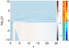Fig. 3. Error of the approximated Voigt function (Eq. (22)) relative to the wofz reference (left; logarithmic) and computational time relative to that of the Gaussian function (right; linear).

3.6. Collision-induced absorption

HITRAN provides tabulated coefficients $k_{\stackrel{\sim }{\nu }}^{(\mathrm{A},\mathrm{B})}$ [cm⁵ molecules⁻²] for a binary collision complex involving species A and B, from which the total absorption coefficient of CIA is computed as

$$\begin{array}{c}\hfill {\alpha }_{\mathrm{CIA}}(\nu ,T)={\displaystyle \sum _{(A,B)}}{k}_{\stackrel{\sim }{\nu }}^{(\mathrm{A},\mathrm{B})}{N}_{\mathrm{A}}{N}_{\mathrm{B}}.\end{array}$$(23)

Here, the coefficients $k_{\stackrel{\sim }{\nu }}^{(\mathrm{A},\mathrm{B})}$ includes the correction factor of induced absorption. In our code, we consider pairs of (A,B) = (H₂,H₂), (H₂,He), (N₂,N₂), (CH₄,He), (CO₂,CH₄), (CO₂,CO₂), (CO₂,H₂), (CO₂,He), (H₂,CH₄), (H₂,H), (He, H), (N₂,H₂O), (N₂,H₂), (N₂,He), (O₂,CO₂), (O₂,O₂), and (O₂,N₂).

3.7. Scattering

With respect to scattering, in addition to Thomson scattering, whose cross-section is

$$\begin{array}{c}\hfill {\sigma }_{\mathrm{T}}={\displaystyle \frac{8\pi }{3}}{\left({\displaystyle \frac{e^2}{m_{\mathrm{e}}{c}^2}}\right)}^2,\end{array}$$(24)

we have implemented the Rayleigh scattering of H in the ground state (Lee 2005), H₂ (Tarafdar & Vardya 1973), and He in the ground state (Rohrmann 2017). Lee (2005) reported an exact low-energy expansion of the cross-section redward of Lyman α. Rohrmann (2017) reported analytical expressions for the cross-section including resonances, with reasonable precision up to the 15th resonance.

We assume that the scattering is isotropic and coherent, in which case, any induced scattering is canceled out between the in- and out-scattering. Then, the scattering coefficient can be written as the sum of the number density N times the scattering cross-section σ^(s):

$$\begin{array}{c}\hfill {\alpha }^{(\mathrm{s})}(\stackrel{\sim }{\nu };T)=N_{\mathrm{e}}{\sigma }_{\mathrm{T}}+{\displaystyle \sum _{i=\mathrm{H},\mathrm{He}}{N_i}_1{\sigma }_i^{(\mathrm{s})}(\stackrel{\sim }{\nu })+N_{{\mathrm{H}}_2}{\sigma }_{{\mathrm{H}}_2}^{(\mathrm{s})}(\stackrel{\sim }{\nu }),}\end{array}$$(25)

where N_i1 ≡ N_ig_i1/Q_i and ${\sigma }_i^{(\text{s})}$ denote the number density in the ground state and the scattering cross-section of species i, respectively.

3.8. Mean opacities

The total absorption coefficient is the sum of all the absorption coefficients described above:

$$\begin{array}{c}\hfill {\alpha }_{\mathrm{total}}\equiv {\alpha }_{\mathrm{bre}}+{\alpha }_{\mathrm{pho}}+{\alpha }_{\mathrm{line}}+{\alpha }_{\mathrm{CIA}},\end{array}$$(26)

where necessary sums related to species and transitions are taken for each term.

The Rosseland mean opacity ${\overline{\alpha }}_{\mathrm{R}}$ and Planck mean opacity ${\overline{\alpha }}_{\mathrm{P}}$ are defined, respectively, as

$$\begin{array}{cc}& {\displaystyle \frac{1}{{\overline{\alpha }}_{\mathrm{R}}(T)}}\equiv \int {\displaystyle \frac{1}{{\alpha }_{\mathrm{total}}(\stackrel{\sim }{\nu };T)+{\alpha }^{(\mathrm{s})}(\stackrel{\sim }{\nu };T)}}{\displaystyle \frac{\partial B_{\stackrel{\sim }{\nu }}(T)}{\partial T}}\mathrm{d}\stackrel{\sim }{\nu }/\int {\displaystyle \frac{\partial B_{\stackrel{\sim }{\nu }}(T)}{\partial T}}\mathrm{d}\stackrel{\sim }{\nu },\hfill \end{array}$$(27)

$$\begin{array}{cc}\hfill & {\overline{\alpha }}_{\mathrm{P}}(T;T_2)\equiv {\displaystyle \frac{\int {\alpha }_{\mathrm{total}}(\stackrel{\sim }{\nu };T)B_{\stackrel{\sim }{\nu }}(T_2)\mathrm{d}\stackrel{\sim }{\nu }}{\int B_{\stackrel{\sim }{\nu }}(T_2)\mathrm{d}\stackrel{\sim }{\nu }}},\hfill \end{array}$$(28)

where T₂ = T (gas temperature) for the normal Planck mean opacity and T₂ = T_rad (external radiation temperature) for the two-temperature Planck mean opacity. $B_{\stackrel{\sim }{\nu }}(T)$ and $\partial B_{\stackrel{\sim }{\nu }}/\partial T$ are, respectively, the Planck function in terms of wavenumber $\stackrel{\sim }{\nu }$ and its temperature derivative:

$$\begin{array}{cc}& B_{\stackrel{\sim }{\nu }}(T)\equiv B_{\nu }(T){\displaystyle \frac{\mathrm{d}\nu }{\mathrm{d}\stackrel{\sim }{\nu }}}=2h{c}^2{\displaystyle \frac{{\stackrel{\sim }{\nu }}^3}{exp(c_2\stackrel{\sim }{\nu }/T)-1}},\hfill \end{array}$$(29)

$$\begin{array}{cc}\hfill & {\displaystyle \frac{\partial B_{\stackrel{\sim }{\nu }}(T)}{\partial T}}=2h{c}^2{\displaystyle \frac{c_2{\stackrel{\sim }{\nu }}^{4}exp(c_2\stackrel{\sim }{\nu }/T)}{T^2{(exp(c_2\stackrel{\sim }{\nu }/T)-1)}^2}},\hfill \end{array}$$(30)

where B_ν(T) is the Planck function in terms of frequency ν. We note that the dependence of the opacities on pressure P is omitted here.

We use the trapezoid rule to evaluate integrals on wavenumber $\stackrel{\sim }{\nu }$ for the Rosseland mean opacity ${\overline{\alpha }}_{\mathrm{R}}$. As for the Planck mean opacity ${\overline{\alpha }}_{\mathrm{P}}$, the integration of absorption coefficients on the wavenumber $\stackrel{\sim }{\nu }$ strongly depends on the grid resolution, particularly for lines. Therefore, while we evaluate the continuum part of the Planck mean opacity using the trapezoid rule on the wavenumber grid, we evaluate the line part as follows (cf. Mayer & Duschl 2005):

$$\begin{array}{c}\hfill {\overline{\alpha }}_{\mathrm{P}}^{\mathrm{line}}(T;T_2)\approx {\displaystyle \frac{{\sum }_{\mathit{lu}}N{x}^{(\mathrm{iso})}{S}_{\mathit{lu}}(1-exp(-c_2{\stackrel{\sim }{\nu }}_{\mathit{ul}}/T))B_{{\stackrel{\sim }{\nu }}_{\mathit{ul}}}(T_2)}{\int B_{\stackrel{\sim }{\nu }}(T_2)\mathrm{d}\stackrel{\sim }{\nu }}},\end{array}$$(31)

which is independent of the wavenumber grid. Here, we assume the line profile ${\varphi }_{\mathit{ul}}(\stackrel{\sim }{\nu })\approx \delta (\stackrel{\sim }{\nu }-{\stackrel{\sim }{\nu }}_{\mathit{ul}})$, and the summation ∑_lu is taken for all the transitions (the summation on the species is omitted for brevity). The validation of this method to evaluate the Planck mean opacity is described in Sect. 5.2.

4. Reducing computational effort in the line opacity calculations

The bottleneck in the opacity calculations is the line absorption, particularly the Voigt profile calculation. This is because computation of the Voigt function K(x, y) requires significant time (e.g., discussion in Schreier 2018), and because the Voigt profile has wide wings and thus the number of grid points over which the function is evaluated is relatively large compared to the Gaussian profile. Ideally, the Voigt profile calculation should be performed for all line transitions at all grid points. However, the number of transitions in the Kurucz atomic line list is several 10⁸, and that in the Exomol database exceeds 10¹⁰ for some species. Clearly, it is not practical to evaluate the line profile for all these transitions over grid points that can easily exceed 10⁵. In reality, not all transitions are strong enough to be evaluated, and the value of opacity may be negligible at grid points far from the line center.

Following the PHOENIX code, we have implemented an algorithm in our code to reduce the number of “Voigt lines”: lines for which the Voigt profile needs to be evaluated. The algorithm is represented by the pseudo code in Algorithm 1. Suppose a line transition whose center and intensity are ${\stackrel{\sim }{\nu }}_{\mathit{ul}}$ and S_lu, respectively. We use the Gaussian profile to evaluate the nominal absorption coefficient at the line center as

$$\begin{array}{c}\hfill {\alpha }_{\mathrm{line}}^{\ast }\equiv {\displaystyle \frac{x^{(\mathrm{iso})}N{S}_{\mathit{lu}}}{\sqrt{\pi }{\sigma }_{\mathrm{G}}}}.\end{array}$$(32)

Then we consider the following ratio:

$$\begin{array}{cc}& \delta \equiv {\displaystyle \frac{{\alpha }_{\mathrm{line}}^{\ast }}{{\alpha }_{\mathrm{cont}}^{\ast }}},\hfill \end{array}$$(33)

$$\begin{array}{cc}\hfill & {\alpha }_{\mathrm{cont}}^{\ast }\equiv {\alpha }_{\mathrm{bre}}({\stackrel{\sim }{\nu }}_{k^{\ast }})+{\alpha }_{\mathrm{pho}}({\stackrel{\sim }{\nu }}_{k^{\ast }})+{\alpha }_{\mathrm{CIA}}({\stackrel{\sim }{\nu }}_{k^{\ast }}).\hfill \end{array}$$(34)

Here ${\alpha }_{\text{cont}}^{*}$ is the continuum absorption coefficient at the grid point (${\stackrel{\sim }{\nu }}_{k^{\ast }}$) nearest to the line center (${\stackrel{\sim }{\nu }}_{\mathit{ul}}$). If δ < δ_crit (typically 10⁻⁴ in our code), we consider the line to be too weak to contribute the total opacity and discard it. If δ > δ_voigt (typically unity in our code), we consider the line to be sufficiently strong and evaluate the Voigt profile at grid points in the range ${\stackrel{\sim }{\nu }}_{\mathit{ul}}-{\mathrm{\Delta }}_{\mathrm{V}}\le \stackrel{\sim }{\nu }\le {\stackrel{\sim }{\nu }}_{\mathit{ul}}+{\mathrm{\Delta }}_{\mathrm{V}}$, where Δ_V is the search window (typically Δ_V = 100 cm⁻¹ in our code). In other cases, where δ_crit < δ < δ_voigt, we consider that only the vicinity of the line center contributes to the total opacity and evaluate the Gaussian profile instead of the Voigt profile (we call this a “Gauss line”). The search window for Gauss lines (typically Δ_G = 3σ_G in our code) is usually much smaller than that for Voigt lines. These values of search windows for Voigt lines and Gauss lines, as well as the values of δ_voigt and δ_crit, are user-defined parameters.

Figure 4 demonstrates how the above algorithm considerably reduces the number of the time-consuming Voigt lines without introducing notable errors into the total opacity and mean opacities. The upper panel shows the dependence on the parameter δ_crit with δ_voigt = 0 fixed; that is, all considered lines are Voigt lines here. (For comparison, the case in which the HITRAN’s dynamic intensity cutoff (Rothman et al. 2013) is used instead of δ_crit is shown in the leftmost.) For example, when δ_crit = 10⁻³, the number of Voigt lines is reduced to 53 % of that in the reference (δ_crit = δ_voigt = 0); however, the error in the mean opacity defined as $\sqrt{{((\overline{\alpha }-{\overline{\alpha }}^{(\mathrm{r})})/{\overline{\alpha }}^{(\mathrm{r})})}^2}$ as well as that in the monochromatic opacity defined as $\sqrt{\sum _k{(\left({\alpha }_k-{\alpha }_k^{(\mathrm{r})}\right)/{\alpha }_k^{(\mathrm{r})})}^2/\sum _k}$ are negligible (specifically, the largest error is 0.0020, occurring in the Rosseland mean opacity). Here, the superscript (r) and the subscript k denote the reference and the grid point index, respectively. The lower panel shows the dependence on the parameter δ_voigt with δ_crit = 10⁻⁴ fixed. For example, when δ_voigt = 1, the number of Voigt lines is reduced to 8% of that in the reference, and the errors are sufficiently low (specifically, the largest error of 0.0042 occurred in the monochromatic opacity).

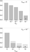Fig. 4. Relative number of the Voigt lines (gray bar) (as well as that of Gauss lines; light gray bar) against the total number of lines in the reference case (δvoigt = δcrit = 0). Also, relative errors of the Rosseland (triangle) and Planck (square) mean opacity as well as of the monochromatic absorption coefficient (filled circle) are plotted. The CE abundance data used here are taken from the first layer of a demo output produced by FASTCHEM, chem_output_agb_stellar_wind.dat. The asterisk in the upper panel indicates a run that employs HITRAN’s dynamic strength cutoff, instead of δcrit.

5. Code validation and performance study

CE abundances for results presented in this section were obtained using the CE solver ACES employed in the PHOENIX code. Here, the element abundance was based on Asplund et al. (2005) and the total number of chemical species considered was 676, which consisted of 428 atomic species (including highly ionized ions) and 248 molecular species.

5.1. Comparison with PHOENIX

For the validation of the code, we compared the mean opacities generated by OPTAB with those generated by PHOENIX. In Fig. 5, the Rosseland mean, Planck mean, and two-temperature Planck mean (at a radiation temperature of 6000 K) opacities are compared as functions of temperature for different total pressures. Here, exactly the same wavenumber grid and CE abundances were used. The opacity sources were chosen from those implemented in both OPTAB and PHOENIX– specifically, Kurucz atomic lines, Rayleigh scattering by H, He, and H₂, and bremsstrahlung and photoionization by atomic ions, including H⁻. The line evaluation parameters described in Sect. 4 are set as δ_crit = 10⁻⁴, δ_voigt = 1, Δ_V = 100 cm⁻¹ (Δ_V = 100 Å for Phoenix runs), and Δ_G = 3σ_G. Moreover, here we use the trapezoid rule to evaluate Planck mean opacities (cf. Sect. 3.8) because PHOENIX uses that method.

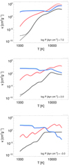Fig. 5. Comparison of mean opacities between OPTAB (thin solid) and PHOENIX (thick): Rosseland mean (black), Planck mean (red), and two-temperature Planck mean for Tred = 6000 K (blue) at log P = 7 (top), log P = 2 (middle), and log P = −3 (bottom). The data represented by the thin dotted curves are explained in the text.

Figure 5 shows that the mean opacities generated by OPTAB basically agree with those generated by PHOENIX. However, there are some discrepancies, particularly in the highest-pressure case (log P = 7), at low temperatures for the Rosseland mean and at high temperatures for the Planck mean. We have identified that the former discrepancy originates from the line profile evaluation, whereas the latter originates from the collisional broadening evaluation. The line profile evaluation is performed in the wavenumber basis in OPTAB, whereas it is performed in the wavelength basis in PHOENIX. As these two bases are identical only near the line center, there may be differences when line profile evaluations are performed for wide ranges. As for the collisional broadening evaluation, when the Kurucz database does not provide the value, OPTAB and PHOENIX calculate it based on slightly different models (cf. Appendix B for the model employed by OPTAB). The difference is notable when the collisional broadening becomes significant at high pressures. When OPTAB employed the same methods as PHOENIX for evaluating the line profile and the collisional broadening, the generated mean opacities, represented by thin dotted curves in Fig. 5, agreed with PHOENIX almost perfectly, as expected.

5.2. Dependence on the number of grid points

In this section, we examine the dependence of mean opacities on the grid parameters. Figure 6 shows the Rosseland mean, Planck mean, and two-temperature Planck mean opacities at log P = 2 as a function of temperature. The opacity sources we adopted here are Kurucz atomic lines, HITRAN and HITEMP molecular lines, Rayleigh scattering by H, He, and H₂, and bremsstrahlung and photoionization by atomic ions, including H⁻ and H₂. The wavenumber grid points were equally spaced on a logarithmic grid covering from 10 to 10⁷ cm⁻¹.

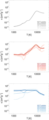Fig. 6. Dependence of Rosseland mean (top), Planck mean (middle), and two-temperature Planck mean for Trad = 6000 K at log P = 2 on the number of grid points, equally spaced on a logarithmic grid. The thick light curves in the middle and the bottom panels are obtained via grid-independent calculations.

In each panel, curves of darker colors correspond to calculations using more grid points, ranging from 10³ to 10⁷. The Rosseland mean opacities (shown in the top panel) are almost identical when the grid points are 10⁴ or more. This is because the Rosseland mean opacities here are basically determined by the continuum sources. In contrast, the Planck mean and the two-temperature Planck mean opacities (shown in the middle and bottom panels, respectively) strongly depend on the number of the grid points because more line opacities are resolved with more grid points. For the Planck mean opacities (middle panel), as many as 10⁶ grid points are required for convergence, whereas convergence is not observed for the two-temperature Planck mean opacities (bottom panel) with 10⁷ or fewer grid points.

To avoid the issue of convergence, OPTAB calculates Planck mean and two-temperature Planck mean opacities for lines in a grid-independent way as described in Sect. 3.8, which are represented by thick light curves in the middle and bottom panels in Fig. 6. As evident from the figures, the grid-independent calculation agrees with a grid-dependent calculation with the largest number of grid points for both Planck mean and two-temperature Planck mean opacities, which validates the method of the grid-independent calculation.

As mentioned in Sect. 4, OPTAB has parameters that determines the grid-search window sizes, Δ_G(=3σ_G) and Δ_V(=100 cm⁻¹), where the values in the parenthesis are code defaults. We also investigated the dependence of the Rosseland mean opacities on these parameters, which was observed to be weak. As mentioned earlier, this is because the Rosseland mean opacities are mainly determined by the continuum sources in the case investigated here.

5.3. MPI parallelization and its performance

In OPTAB, MPI parallelization on the layer loop (Fig. 1) has been implemented. The parallelization performance is shown in Fig. 7 against the mean opacity calculations for 64 layers in total (composed of 8 grid points both in the temperature and pressure grids as shown in Fig. 8). The opacity sources were the same as those described in Sect. 5.2, and the number of the wavenumber grid points for computing the Rosseland mean opacities was 10⁵. The code parameters used were δ_crit = 10⁻⁴, δ_voigt = 1, Δ_G = 3σ_G, and Δ_V = 100 cm⁻¹.

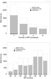Fig. 7. MPI parallel performance for parallelization on the layer loop (upper) and the load balance in the case of 8 MPI processes (lower). The white, gray, and black bars correspond, respectively, to the wall times for atomic lines, molecular lines, and continuum. The computation was performed, using gfortran 10.2 + Open MPI 4.1 + HDF5 1.12, on 2.3 GHz 8-Core Intel Core i9 processors.

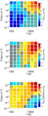Fig. 8. Rosseland mean (top), Planck mean (middle), and two-temperature Planck mean (bottom) opacities on the temperature–pressure grid composed of 64 points (layers).

The dependence of the wall time on the number of MPI processes is shown in the upper panel in Fig. 7. While the computation on each MPI process is independent (i.e., no message passing is necessary), it is often difficult to achieve the load balance between the MPI processes, as shown in the lower panel. This is because the most time-consuming part (i.e., the computation of line opacities) can differ significantly between the layers. Hence, the parallel performance becomes worse as the number of processes increases. We will attempt to improve the parallel performance in the future version of the code.

6. Discussion on future aspects

As demonstrated in the previous section, we have successfully developed a code that generates mean opacity tables. The main features are that the code is public and runs based on the user’s choice of CE abundances, opacity sources, and sampling grid. In this section, we discuss some aspects that remain for future work.

Including dust opacities in our code is obviously the next target. We did not include them in the first version of our code because they depend on a dust model, which has not yet been established. In addition, the degree to which the dust abundances are involved in the CE of the gas mixture is not trivial. (If the dust abundances are independent from the CE of the gas mixture, one may simply add dust opacities taken from the literature (e.g., Semenov et al. 2003) to the gas opacities computed by our code, assuming some dust-to-gas mass ratio.) We need to solve these issues in order to include dust opacities.

There are a few issues related to line broadening, although they may not affect the mean opacities. For example, we left implementing the linear Stark effect for hydrogen atoms (e.g., Sect. 8.2.8 in Hertel & Schulz 2014) as future work. We are planning to use the tables provided in Stehlé & Hutcheon (1999), Stehlé & Fouquet (2010) to implement the linear Stark effect. Another issue is that pressure broadening parameters are not always provided together with a line list. If not provided, we can evaluate them for atoms using the (semi-)classical theory described in Appendix B. However, we are not aware of a proper way to evaluate them for molecules.

Finally, the opacity sources implemented in the first version of the code are basic ones. We will continue to compile additional opacity sources to enhance our code, and we also expect to receive user contributions via GitHub.

Acknowledgments

We thank the anonymous referee for his/her valuable comments to improve our manuscript as well as our code. This work was supported by JSPS KAKENHI (Grant Number JP18K03716). P.H.H. gratefully acknowledges support from the DFG under grants HA 3457/20-1 and HA 3457/23-1. P. H. H. gratefully acknowledges the support of NVIDIA Corporation with the donation of the Quadro P6000 GPU used in this research.

References

Appendix A: Data conversions of line lists into the HDF5 format

For flexible and efficient I/O of very large atomic or molecular line lists (Kurucz, HITRAN, and Exomol), their original ASCII files are converted into HDF5 files beforehand. Furthermore, the atomic properties in ASCII format collected from NIST ASD/AWIC, TOPbase energy levels and photoionization cross-sections, and HITRAN CIA data are converted into a single HDF5 file, respectively. Programs for these conversions to HDF5 (written in Fortran 2003) are associated with the code package. Table A.1 summarizes the external sources for the isotope or isotopologue fraction, partition function, and mass that are needed for making these HDF5 files. The structure of the HITRAN CIA file in HDF5 format is simple and thus is not explained here.

A.1. NIST atomic property file in HDF5 format

Fig. A.1 depicts the data structure in the NIST atomic property file in HDF5 format. The data sets nstates, term, ene, gtot, and eneion are taken from the NIST ASD levels form, whereas mass is taken from NIST AWIC.

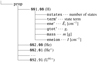Fig. A.1. Structure of the NIST atomic property file in HDF5 format. Data sets with asterisks are arrays of size nstates.

A.2. Kurucz atomic line lists in HDF5 format

In the Kurucz database, there are two categories of line lists for atoms, “gfall” and “gfpred.” All lines in the gfall files are based on laboratory-measured energy levels, while the gfpred files contain only predicted lines to complement the gfall files. In Sect. 5, we used both kinds of the line lists.

In the Kurucz line lists, each line transition is labeled by its species code¹⁷, and for each line transition, ${\stackrel{\sim }{E}}_l$, ${\stackrel{\sim }{E}}_u$, log(g_lf_lu) and $log{x}_{lu}^{\text{(iso)}}$, as well as $\mathrm{\Delta }{\stackrel{\sim }{E}}_l$, $\mathrm{\Delta }{\stackrel{\sim }{E}}_u$, and Δlog(g_lf_lu) are provided. The quantities including Δ are corrections required because of hyperfine shifts. The wavenumber of the line transition is then calculated as

$$\begin{array}{c}\hfill {\stackrel{\sim }{\nu }}_{\mathit{ul}}=\left(|{\stackrel{\sim }{E}}_u|+\mathrm{\Delta }{\stackrel{\sim }{E}}_u\right)-\left(|{\stackrel{\sim }{E}}_l|+\mathrm{\Delta }{\stackrel{\sim }{E}}_l\right),\end{array}$$(A.1)

where absolute values are used for ${\stackrel{\sim }{E}}_u$ and ${\stackrel{\sim }{E}}_l$, because in the Kurucz line lists, the level energies have a negative sign when the involving line transition is a predicted (not a measured) one.

Isotopic shifts in energy levels are miniscule for most atoms, for which the Kurucz line lists do not include distinct isotopes, where $log{x}_{lu}^{\text{(iso)}}=0$. However, there are a small number of strong lines whose isotopic shifts have been measured in laboratories. In Kurucz’s line lists, such lines are indicated by a finite value of $log{x}_{lu}^{\text{(iso)}}$. Therefore, we redefine the g-f values by considering the hyperfine and isotopic shifts as

$$\begin{array}{c}\hfill {(g_l{f}_{\mathit{lu}})}^{\prime }={10}^{log(g_l{f}_{\mathit{lu}})+\mathrm{\Delta }log(g_l{f}_{\mathit{lu}})+log{x}_{\mathit{lu}}^{\text{(iso)}}}\end{array}$$(A.2)

and use this relationship to compute the absorption coefficient (cf. Eq. 12):

$$\begin{array}{cc}\hfill {\displaystyle \frac{{\alpha }_{\text{line}}^{\text{Kurucz}}(\stackrel{\sim }{\nu })}{N}}& =S_{\mathit{lu}}^{\prime }{\varphi }_{\mathit{ul}}(\stackrel{\sim }{\nu }),\hfill \end{array}$$(A.3)

$$\begin{array}{cc}\hfill S_{\mathit{lu}}^{\prime }& \equiv \left({\displaystyle \frac{\pi e^2}{m_{\mathrm{e}}{c}^2}}\right){(g_l{f}_{\mathit{lu}})}^{\prime }{\displaystyle \frac{{\mathrm{e}}^{-c_2{\stackrel{\sim }{E}}_l/T}}{Q(T)}}(1-{\mathrm{e}}^{-c_2{\stackrel{\sim }{\nu }}_{\mathit{ul}}/T}).\hfill \end{array}$$(A.4)

Because the Kurucz line lists have some incorrect values of $log{x}_{lu}^{\text{(iso)}}$, we replace them in Eq. (A.2) with those computed from the NIST AWIC (Table A.1).

For line broadening, the Kurucz line lists provide three damping constants (in terms of the angular frequency ω), the natural damping constant ${\mathrm{\Gamma }}_{\text{nat}}^{(\omega )}$ [s⁻¹], the quadratic Stark damping constant (divided by the free electron number density) ${\mathrm{\Gamma }}_{\text{Stark}}^{(\omega )}/N_{\text{e}}$, and the damping constant of van der Waals broadening by H atoms (divided by the atomic hydrogen number density) ${\mathrm{\Gamma }}_{\text{vdW}}^{(\omega )}/N_{\text{H}}$. The total Lorentzian half-width in terms of the wavenumber is then calculated as

$$\begin{array}{c}\hfill \gamma ={\displaystyle \frac{1}{2}}{\displaystyle \frac{1}{2\pi c}}({\mathrm{\Gamma }}_{\text{nat}}^{(\omega )}+\left({\displaystyle \frac{{\mathrm{\Gamma }}_{\text{Stark}}^{(\omega )}}{N_{\text{e}}}}\right)N_{\text{e}}+\left({\displaystyle \frac{{\mathrm{\Gamma }}_{\text{vdW}}^{(\omega )}}{N_{\text{H}}}}\right)N_{\text{H}}).\end{array}$$(A.5)

Fig. A.2 depicts the data structure in the Kurucz line list in HDF5 format. It shows that the quantities necessary for calculating the line opacity Eq. (A.3) are stored in the data sets wnum, lowe, gfva, gm_0, gm_1, and gm_2 in the group trans. The data set rsqd is used in Eq. (B.4) in Appendix B. The data set code is necessary to identify the species of each line since the line transitions of all the species are stored in a single file. The partition function for each species is computed from the NIST energy level data, that is, data sets ene and gtot stored in the NIST HDF5 file (Fig. A.1). This is because, in the Kurucz line lists, partition functions computed from all measured and predicted levels are provided, but only for a limited number of species.

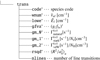Fig. A.2. Structure of the Kurucz atomic line list in HDF5 format. Data sets with asterisks are arrays of size nlines.

A.3. HITRAN and Exomol molecular line lists in HDF5 format

Because the isotopic shifts can be significant in molecules, the line list and the partition function table are provided for each isotopologue in databases HITRAN and Exomol. As for the isotopologue abundances x^(iso), HITRAN provides them separately from the line list as “Isotopologue Metadata”¹⁸ while Exomol does not provide them. Therefore, for Exomol, we compute x^(iso) using NIST AWIC (Table A.1), assuming the terrestrial isotopic abundances of elements.

The HITRAN and Exomol line lists give the Einstein coefficients A_ul and statistical weights g_u, from which the g-f value is calculated as

$$\begin{array}{c}\hfill \left(g_l{f}_{\mathit{lu}}\right)={\displaystyle \frac{c{m}_{\mathrm{e}}}{8{\pi }^2{e}^2{\stackrel{\sim }{\nu }}_{\mathit{ul}}^2}}{A}_{\mathit{ul}}{g}_u.\end{array}$$(A.6)

For line broadening, HITRAN and Exomol consider the van der Waals broadening only and employ the same convention to compute the corresponding Lorentzian half-width as a function of temperature T and the perturber’s partial pressure p as

$$\begin{array}{c}\hfill {\gamma }_{\mathrm{vdW}}(p,T)={\left({\displaystyle \frac{T_{\mathrm{ref}}}{T}}\right)}^n{\gamma }_{\mathrm{vdW},\mathrm{ref}}\left({\displaystyle \frac{p}{p_{\mathrm{ref}}}}\right),\end{array}$$(A.7)

where T_ref = 296 K and p_ref = 1 ([atm] in HITRAN and [bar] in Exomol) are the reference temperature and pressure, respectively. The exponent n and the reference width γ_{vdW,  ref} ≡ γ_vdW(p_ref, T_ref) [cm⁻¹] are parameters given in the line list and depend on the perturbers considered. Both HITRAN and Exomol consider two kinds of perturbers for broadening: HITRAN considers air (p = p_total − p_self) and self (p = p_self) broadening, while Exomol considers, in most cases, broadening by H₂ molecules (p = p_H2) and by He atoms (p = p_He). In our code, we determine the total Lorentzian half-width considering both the natural broadening (Eq. 20) and the van der Waals broadening by the two kinds of perturbers:

$$\begin{array}{c}\hfill \gamma ={\gamma }_{\mathrm{nat}}+{\gamma }_{\mathrm{vdW}}^{\#1}+{\gamma }_{\mathrm{vdW}}^{\#2}.\end{array}$$(A.8)

Here, the perturbers {#1, #2} denote, respectively, {“air”, “self”} for HITRAN and {H₂, He} for Exomol.

The structure of the molecular line list in HDF5 format for a single molecular species is shown in Fig. A.3. The species is identified by the data set id in the group prop. The quantities necessary to compute the line opacity (Eq. 12) are stored in the data sets in groups prop and trans. The former contains quantities specific to the species while the latter contains those specific to the line. The partition function is calculated by the linear interpolation of the table provided with the line list, which is stored in the data set pf in the group prop. When the temperature to be considered is not within the data set temp, the temperature range of the partition function, the line absorption is not considered, as described in line 8 of Algorithm 1.

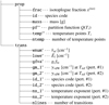Fig. A.3. Structure of molecular line list in HDF5 format. Data sets with asterisks are arrays of size nlines, whereas those with double asterisks are arrays of size ntemp.

Appendix B: Calculation of collisional damping widths for atomic lines

Here we describe how to calculate collisional damping widths for atomic lines when they are not given in the Kurucz atomic line lists. We consult NIST ASD/AWIC for the ionization energy and mass of atoms, which are quantities required to calculate the line broadening parameters in this section.

B.1. Quadratic Stark broadening

According to a semi-empirical formula in Griem (1974, Eqs. 459, 460),

$$\begin{array}{cc}\hfill {\displaystyle \frac{{\mathrm{\Gamma }}_{\text{Stark}}^{(\omega )}}{2}}& =8{\left({\displaystyle \frac{\pi }{3}}\right)}^{\frac{3}{2}}{\displaystyle \frac{ħa_0}{m}}{N}_{\text{e}}{\left({\displaystyle \frac{I_{\text{H}}}{k_{\mathrm{B}}T}}\right)}^{\frac{1}{2}}\hfill \\ \hfill & ({⟨{\displaystyle \frac{R^2}{a_0^2}}⟩}_{u}g\left({\displaystyle \frac{3k_{\mathrm{B}}T}{2\mathrm{\Delta }{E}_u}}\right)+{⟨{\displaystyle \frac{R^2}{a_0^2}}⟩}_{l}g\left({\displaystyle \frac{3k_{\mathrm{B}}T}{2\mathrm{\Delta }{E}_l}}\right)),\hfill \end{array}$$(B.1)

where I_H is the ionization energy of hydrogen, and ΔE_i is the perturbed energy in state i due to a collision. The radiator’s effective radius squared (in terms of the Bohr radius a₀) in state i is evaluated as

$$\begin{array}{c}\hfill {⟨{\displaystyle \frac{R^2}{a_0^2}}⟩}_i={\displaystyle \frac{1}{2}}{\left({\displaystyle \frac{n_i^{\ast }}{Z+1}}\right)}^2[5{n_i^{\ast }}^2+1-3l_i(l_i+1)].\end{array}$$(B.2)

Here, l_i is the orbital quantum number of the valence electron in state i, and the effective principal quantum number in state i is defined as

$$\begin{array}{c}\hfill n_i^{\ast }=(Z+1){\left({\displaystyle \frac{I_{\text{H}}}{I-E_i}}\right)}^{\frac{1}{2}},\end{array}$$(B.3)

where Z, I, and E_i are the charge number, the ionization energy, and the energy in state i of the radiator, respectively.

In our code, for simplicity, we employ the following approximations:

$$\begin{array}{cc}& {⟨{\displaystyle \frac{R^2}{a_0^2}}⟩}_i\approx {\displaystyle \frac{5}{2}}{\displaystyle \frac{{n_i^{\ast }}^4}{{(Z+1)}^2}},\hfill \end{array}$$(B.4)

$$\begin{array}{cc}\hfill & g(x)\approx 0.2.\hfill \end{array}$$(B.5)

The approximation given by Eq. (B.5) is based on the discussion above pertaining to Eq. 459 in Griem (1974).

B.2. van der Waals broadening

According to the Lindholm approximation in classical impact theory (e.g., p.258 in Mihalas 1970),

$$\begin{array}{cc}\hfill {\displaystyle \frac{{\mathrm{\Gamma }}_{\text{vdW}}^{(\omega )}}{2}}& =N_{\text{pert}}{v}_{\text{pert}}{\int }_0^{\infty }\rho (1-cos\left({\displaystyle \frac{(3\pi /8)C_6}{v{\rho }^5}}\right))d\rho \hfill \\ \hfill & =f{C}_6^{\frac{2}{5}}{v}_{\text{pert}}^{\frac{3}{5}}{N}_{\text{pert}},\hfill \end{array}$$(B.6)

$$\begin{array}{cc}\hfill & f\equiv -(1+\sqrt{5})\mathrm{\Gamma }(-{\displaystyle \frac{2}{5}}){\displaystyle \frac{\pi }{5}}{\left({\displaystyle \frac{3\pi }{8}}\right)}^{\frac{2}{5}}\approx 8.08,\hfill \end{array}$$(B.7)

where N_pert and v_pert are the number density and the velocity of the perturber, respectively, and Γ(x) is the Gamma function. Based on quantum theory (e.g., p.297 in Mihalas 1970), the factor C₆ is evaluated as

$$\begin{array}{c}\hfill C_6={\displaystyle \frac{e^2{a}_0^2}{ħ}}{\alpha }_{\text{pert}}^{(\text{pol})}({⟨{\displaystyle \frac{R^2}{a_0^2}}⟩}_u-{⟨{\displaystyle \frac{R^2}{a_0^2}}⟩}_l),\end{array}$$(B.8)

where ${\alpha }_{\text{pert}}^{(\text{pol})}$ is the polarizability of the perturber.

In our code, we evaluate the velocity of the perturber as

$$\begin{array}{c}\hfill v_{\text{pert}}=\sqrt{{v^2}_{\text{pert}}}=\sqrt{{\displaystyle \frac{3k_{\mathrm{B}}T}{m_{\text{pert}}^{\ast }}}},\end{array}$$(B.9)

where ⟨⟩ denotes the thermal average and $m_{\text{pert}}^{*}$ is the reduced mass of the perturber with the radiator. Although we have implemented van der Waals broadening caused only by atomic hydrogen, molecular hydrogen, and helium (Schwerdtfeger & Nagle 2019; Wilkins & Taylor 1968), it is straightforward to add broadening caused by other species if $\left\{v_{\text{pert}},N_{\text{pert}},{\alpha }_{\text{pert}}^{(\text{pol})}\right\}$ are available.

It is known that the damping constant evaluated in the above requires some correction. In our code, we multiply ${\mathrm{\Gamma }}_{\text{vdW}}^{(\omega )}$ by a correction factor of 2.5 based on Valenti & Piskunov (1996).

Appendix C: Partition function, chemical potential, and thermochemical database

In this section, for reference, we summarize the relationships among the partition function, chemical potential, and thermochemical database.

Chemical equilibrium is obtained by minimizing the Gibbs free energy [J mol⁻¹] of the system:

$$\begin{array}{c}\hfill G(T,P)={\displaystyle \sum _i{x}_i{\mu }_i(T,P),}\end{array}$$(C.1)

where x is the molar fraction and index i denotes the species. In the chemical equilibrium calculation, the chemical potential μ [J mol⁻¹] is usually computed from thermochemical databases as (e.g., Eq.(3.12-5a) in Smith & Missen 1982)

$$\begin{array}{c}\hfill \mu (T,P)=RTln\left({\displaystyle \frac{P}{P^{°}}}\right)+RT\{\mathrm{\Delta }{H}_{\text{f}}^{°}(298)-T(-{\displaystyle \frac{G^{°}(T)-H^{°}(298)}{T}})\},\end{array}$$(C.2)

where H indicates the total enthalpy and ΔH_f indicates the enthalpy of formation, and the superscript ° denotes the standard pressure. The quantities ΔH°_f(298) and −(G°(T)−H°(298))/T are provided in thermochemical databases such as NIST-JANAF or NASA CEA. We note that the values of the chemical potential, Eq. (C.2), and Eq. (3) differ by a constant because different values of the zero energy are considered.

The partition function Q(T) can be computed using thermochemical databases. Hereafter we consider the standard pressure. For a pure substance, because the chemical potential is equal to the Gibbs free energy, Eq. (3) can be written as (Eq. (24.50) in McQuarrie & Simon 1997)

$$\begin{array}{c}\hfill G^{°}(T)-H^{°}(0)=RTln\left({\displaystyle \frac{P^{°}}{k_{\mathrm{B}}T}}{\left({\displaystyle \frac{h^2}{2\pi m{k}_{\mathrm{B}}T}}\right)}^{\frac{3}{2}}{\displaystyle \frac{1}{Q(T)}}\right).\end{array}$$(C.3)

Then, the partition function is computed as

$$\begin{array}{cc}\hfill lnQ(T)& =\{-{\displaystyle \frac{3}{2}}ln\left({\displaystyle \frac{m}{m_{\text{u}}}}\right)-{\displaystyle \frac{5}{2}}ln\left({\displaystyle \frac{T}{T_1}}\right)-({\displaystyle \frac{S_0}{R}}-{\displaystyle \frac{5}{2}})\}\hfill \\ \hfill & +\mathit{black}\{-{\displaystyle \frac{G^{°}(T)-H^{°}(298)}{T}}\}{\displaystyle \frac{1}{R}}+{\displaystyle \frac{\mathit{black}\{H^{°}(0)-H^{°}(298)\}}{\mathit{RT}}},\hfill \\ \hfill \end{array}$$(C.4)

where m_u is the atomic mass unit, T₁ = 1 K, and

$$\begin{array}{c}\hfill {\displaystyle \frac{S_0}{R}}\equiv ln\left\{{\left({\displaystyle \frac{2\pi m_{\text{u}}{k}_{\mathrm{B}}{T}_1}{h^2}}\right)}^{\frac{3}{2}}{\displaystyle \frac{k_{\mathrm{B}}{T}_1}{P^{°}}}\right\}+{\displaystyle \frac{5}{2}}=-1.15170753706\end{array}$$(C.5)

is the Sackur-Tetrode constant. The quantity H° (0)−H° (298) is provided in thermochemical databases.

We note that the partition functions computed by Eq. (C.4) differ by a factor of the nuclear partition function from those provided with the corresponding line list, such as HITRAN or Exomol (Hanson et al. 2015). This is because the nuclear partition function is included in the total partition function in the line lists, but is not in the thermochemical databases (Sousa-Silva et al. 2014). We also note that the atomic partition functions in our code, which are computed from the NIST ADS levels form, do not include the nuclear partition function.

All Tables

All Figures

	Fig. 1. Flowchart of OPTAB. The external files in the gray boxes are in the HDF5 format, which have been converted from their original ASCII files (Appendix A).
In the text

Fig. 2. Magnesium photoionization absorption coefficients per Mg atom [cm2] at 5000 K. The brown curve indicates the photoionization from the ground level, and is a hybrid of Verner et al. (1996) (outer-subshell contributions; yellow) and Verner & Yakovlev (1995) (inner-subshell contributions; cyan). Both the magenta and black thin curves indicate the photoionization from excited levels; the former is based on the Mathisen (1984) compilation, whereas the latter is based on TOPbase.

In the text

	Fig. 3. Error of the approximated Voigt function (Eq. (22)) relative to the wofz reference (left; logarithmic) and computational time relative to that of the Gaussian function (right; linear).
In the text

Fig. 4. Relative number of the Voigt lines (gray bar) (as well as that of Gauss lines; light gray bar) against the total number of lines in the reference case (δvoigt = δcrit = 0). Also, relative errors of the Rosseland (triangle) and Planck (square) mean opacity as well as of the monochromatic absorption coefficient (filled circle) are plotted. The CE abundance data used here are taken from the first layer of a demo output produced by FASTCHEM, chem_output_agb_stellar_wind.dat. The asterisk in the upper panel indicates a run that employs HITRAN’s dynamic strength cutoff, instead of δcrit.

In the text

	Fig. 5. Comparison of mean opacities between OPTAB (thin solid) and PHOENIX (thick): Rosseland mean (black), Planck mean (red), and two-temperature Planck mean for Tred = 6000 K (blue) at log P = 7 (top), log P = 2 (middle), and log P = −3 (bottom). The data represented by the thin dotted curves are explained in the text.
In the text

	Fig. 6. Dependence of Rosseland mean (top), Planck mean (middle), and two-temperature Planck mean for Trad = 6000 K at log P = 2 on the number of grid points, equally spaced on a logarithmic grid. The thick light curves in the middle and the bottom panels are obtained via grid-independent calculations.
In the text

	Fig. 7. MPI parallel performance for parallelization on the layer loop (upper) and the load balance in the case of 8 MPI processes (lower). The white, gray, and black bars correspond, respectively, to the wall times for atomic lines, molecular lines, and continuum. The computation was performed, using gfortran 10.2 + Open MPI 4.1 + HDF5 1.12, on 2.3 GHz 8-Core Intel Core i9 processors.
In the text

	Fig. 8. Rosseland mean (top), Planck mean (middle), and two-temperature Planck mean (bottom) opacities on the temperature–pressure grid composed of 64 points (layers).
In the text

	Fig. A.1. Structure of the NIST atomic property file in HDF5 format. Data sets with asterisks are arrays of size nstates.
In the text

	Fig. A.2. Structure of the Kurucz atomic line list in HDF5 format. Data sets with asterisks are arrays of size nlines.
In the text

	Fig. A.3. Structure of molecular line list in HDF5 format. Data sets with asterisks are arrays of size nlines, whereas those with double asterisks are arrays of size ntemp.
In the text

References

- Alexander, D. R. 1975, ApJS, 29, 363 [NASA ADS] [CrossRef] [Google Scholar]
- Alexander, D. R., & Ferguson, J. W. 1994, ApJ, 437, 879 [NASA ADS] [CrossRef] [Google Scholar]
- Alexander, D. R., Johnson, H. R., & Rypma, R. L. 1983, ApJ, 272, 773 [NASA ADS] [CrossRef] [Google Scholar]
- Allard, F., & Hauschildt, P. H. 1995, ApJ, 445, 433 [NASA ADS] [CrossRef] [Google Scholar]
- Aller, L. H., Appenzeller, I., Baschek, B., et al. 1982, "Landolt-Börnstein: Numerical Data and Functional Relationships in Science and Technology - New Series" Gruppe/Group 6 Astronomy and Astrophysics "Volume 2 Schaifers/Voigt: Astronomy and Astrophysics / Astronomie und Astrophysik" Stars and Star Clusters / Sterne und Sternhaufen, 2, 54 [Google Scholar]
- Asplund, M., Grevesse, N., & Sauval, A. J. 2005, Cosmic Abundances as Records of Stellar Evolution and Nucleosynthesis in honor of David L. Lambert, 336, 25 [NASA ADS] [Google Scholar]
- Bell, K. R., & Lin, D. N. C. 1994, ApJ, 427, 987 [NASA ADS] [CrossRef] [Google Scholar]
- Berglund, M., & Wieser, M. E. 2011, Pure Appl. Chem., 83, 397 [CrossRef] [Google Scholar]
- Blecic, J., Harrington, J., & Bowman, M. O. 2016, ApJS, 225, 4 [CrossRef] [Google Scholar]
- Bradley, D. J., Dugan, C. H., Ewart, P., & Purdie, A. F. 1976, Phys. Rev. A, 13, 1416 [CrossRef] [Google Scholar]
- Carson, T. R., Mayers, D. F., & Stibbs, D. W. N. 1968, MNRAS, 140, 483 [NASA ADS] [CrossRef] [Google Scholar]
- Castelli, F. 2005, Mem. Soc. Astron. It. Suppl., 8, 34 [Google Scholar]
- Chapman, R. D. 1969, J. Quant. Spectr. Rad. Transf., 9, 315 [NASA ADS] [CrossRef] [Google Scholar]
- Chapman, R. D. 1970, J. Quant. Spectr. Rad. Transf., 10, 1151 [NASA ADS] [CrossRef] [Google Scholar]
- Chase, M. W. J. 1998, NIST-JANAF Thermochemical Tables (American Institute of Physics) [Google Scholar]
- Cox, A. N., & Stewart, J. N. 1970a, ApJS, 19, 243 [NASA ADS] [CrossRef] [Google Scholar]
- Cox, A. N., & Stewart, J. N. 1970b, ApJS, 19, 261 [NASA ADS] [CrossRef] [Google Scholar]
- Cunto, W., & Mendoza, C. 1992, Rev. Mex. Astron. Astrofis., 23 [Google Scholar]
- Draine, B. T. 2011, in Physics of the Interstellar and Intergalactic Medium, ed. Bruce T. Draine (Princeton University Press), Physics of the Interstellar and Intergalactic Medium [CrossRef] [Google Scholar]
- Ferguson, J. W., Alexander, D. R., Allard, F., et al. 2005, ApJ, 623, 585 [Google Scholar]
- Freedman, R. S., Marley, M. S., & Lodders, K. 2008, ApJS, 174, 504 [NASA ADS] [CrossRef] [Google Scholar]
- Gordon, I. E., Rothman, L. S., Hill, C., et al. 2017, J. Quant. Spectr. Rad. Transf., 203, 3 [Google Scholar]
- Griem, H. R. 1974, Spectral Line Broadening by Plasmas (New York: Academic Press) [Google Scholar]
- Hanson, R. K., Spearrin, R. M., & Goldenstein, C. S. 2015, Spectroscopy and Optical Diagnostics for Gases (Springer) [Google Scholar]
- Hauschildt, P. H., & Baron, E. 1999, J. Comput. Appl. Math., 109, 41 [NASA ADS] [CrossRef] [Google Scholar]
- Helling, C., & Lucas, W. 2009, MNRAS, 398, 985 [NASA ADS] [CrossRef] [Google Scholar]
- Helling, C., Winters, J. M., & Sedlmayr, E. 2000, A&A, 358, 651 [NASA ADS] [Google Scholar]
- Henning, T., & Stognienko, R. 1996, A&A, 311, 291 [NASA ADS] [Google Scholar]
- Hertel, I. V., & Schulz, C.-P. 2014, Atoms, Molecules and Optical Physics 1, (Springer) [Google Scholar]
- Hirose, S., & Shi, J.-M. 2019, MNRAS, 485, 266 [Google Scholar]
- Hirose, S., Blaes, O., Krolik, J. H., Coleman, M. S. B., & Sano, T. 2014, ApJ, 787, 1 [NASA ADS] [CrossRef] [Google Scholar]
- Hoof, P. A. M. V., Williams, R. J. R., Volk, K., et al. 2014, MNRAS, 444, 420 [NASA ADS] [CrossRef] [Google Scholar]
- John, T. L. 1975, MNRAS, 172, 305 [NASA ADS] [Google Scholar]
- John, T. L. 1978, A&A, 67, 395 [NASA ADS] [Google Scholar]
- John, T. L. 1988, A&A, 193, 189 [NASA ADS] [Google Scholar]
- Karzas, W. J., & Latter, R. 1961, ApJS, 6, 167 [Google Scholar]
- Kramida, A., Ralchenko, Y., Reader, J., & NIST ASD Team 2020, NIST Atomic Spectra Database (version 5.8) [Google Scholar]
- Lee, H.-W. 2005, MNRAS, 358, 1472 [NASA ADS] [CrossRef] [Google Scholar]
- Malygin, M. G., Kuiper, R., Klahr, H., Dullemond, C. P., & Henning, T. 2014, A&A, 568, A91 [NASA ADS] [CrossRef] [EDP Sciences] [Google Scholar]
- Mathisen, R. 1984, Photo Cross Sections for Stellar Atmosphere Calculations - Compilation of references and data, Tech. rep. [Google Scholar]
- Mayer, M., & Duschl, W. J. 2005, MNRAS, 358, 614 [NASA ADS] [CrossRef] [Google Scholar]
- Mcbride, B. J., & Gordon, S. 1992, NASA Ref. Publ., 1271 [Google Scholar]
- McQuarrie, D. A., & Simon, J. D. 1997, Physical chemistry: a molecular approach (Sausalito, Calif: University Science Books) [Google Scholar]
- Meija, J., Coplen, T. B., Berglund, M., et al. 2016, Pure Appl. Chem., 88, 265 [Google Scholar]
- Mihalas, D. 1970, Stellar atmospheres, Series of Books in Astronomy and Astrophysics (San Francisco: Freeman) [Google Scholar]
- Ohmura, T., & Ohmura, H. 1960, Phys. Rev., 118, 154 [CrossRef] [Google Scholar]
- Pollack, J. B., Hollenbach, D., Beckwith, S., et al. 1994, ApJ, 421, 615 [Google Scholar]
- Rogers, F. J., & Iglesias, C. A. 1992, ApJ, 401, 361 [NASA ADS] [CrossRef] [Google Scholar]
- Rohrmann, R. D. 2017, MNRAS, 473, 457 [Google Scholar]
- Rothman, L. S., Gordon, I. E., Babikov, Y., et al. 2013, J. Quant. Spectr. Rad. Transf., 130, 4 [Google Scholar]
- Rybicki, G. B., & Lightman, A. P. 2008, Radiative Processes in Astrophysics (John Wiley & Sons) [Google Scholar]
- Schreier, F. 2018, MNRAS, 479, 3068 [NASA ADS] [CrossRef] [Google Scholar]
- Schwerdtfeger, P., & Nagle, J. K. 2019, Mol. Phys., 477, 1 [Google Scholar]
- Seaton, M. J., Zeippen, C. J., Tully, J. A., et al. 1992, Rev. Mex. Astron. Astrofis., 23 [Google Scholar]
- Semenov, D., Henning, T., Helling, C., Ilgner, M., & Sedlmayr, E. 2003, A&A, 410, 611 [NASA ADS] [CrossRef] [EDP Sciences] [Google Scholar]
- Sharp, C. M. 1992, A&AS, 94, 1 [NASA ADS] [Google Scholar]
- Smith, W. R., & Missen, R. W. 1982, Chemical Reaction Equilibrium Analysis (John Wiley& Sons Incorporated) [Google Scholar]
- Sousa-Silva, C., Hesketh, N., Yurchenko, S. N., Hill, C., & Tennyson, J. 2014, J. Quant. Spectr. Rad. Transf., 142, 66 [NASA ADS] [CrossRef] [Google Scholar]
- Stehlé, C., & Fouquet, S. 2010, Int. J. Spectrosc., 2010, 1 [CrossRef] [Google Scholar]
- Stehlé, C., & Hutcheon, R. 1999, A&AS, 140, 93 [NASA ADS] [CrossRef] [EDP Sciences] [Google Scholar]
- Stock, J. W., Kitzmann, D., Patzer, A. B. C., & Sedlmayr, E. 2018, MNRAS, 479, 865 [NASA ADS] [Google Scholar]
- Tarafdar, S. P., & Vardya, M. S. 1973, MNRAS, 163, 261 [CrossRef] [Google Scholar]
- Tennyson, J., & Yurchenko, S. N. 2012, MNRAS, 425, 21 [Google Scholar]
- Thompson, D. G., Hibbert, A., & Chandra, N. 1974, J. Phys. B: At. Mol. Phys., 7, 1298 [NASA ADS] [CrossRef] [Google Scholar]
- Valenti, J. A., & Piskunov, N. 1996, A&AS, 118, 595 [NASA ADS] [CrossRef] [EDP Sciences] [Google Scholar]
- Vernazza, J. E., Avrett, E. H., & Loeser, R. 1976, ApJS, 30, 1 [Google Scholar]
- Vernazza, J. E., Avrett, E. H., & Loeser, R. 1981, ApJS, 45, 635 [Google Scholar]
- Verner, D. A., & Yakovlev, D. G. 1995, A&AS, 109, 125 [NASA ADS] [Google Scholar]
- Verner, D. A., Ferland, G. J., & Korista, K. T. 1996, ApJ, 465, 487 [NASA ADS] [CrossRef] [Google Scholar]
- Wilkins, R. L., & Taylor, H. S. 1968, J. Chem. Phys., 48, 4934 [NASA ADS] [CrossRef] [Google Scholar]
- Yan, M., Sadeghpour, H. R., & Dalgarno, A. 2001, ApJ, 559, 1194 [NASA ADS] [CrossRef] [Google Scholar]
- Yurchenko, S. N., Al-Refaie, A. F., & Tennyson, J. 2018, A&A, 614, A131 [NASA ADS] [CrossRef] [EDP Sciences] [Google Scholar]