| Issue |
A&A
Volume 658, February 2022
|
|
|---|---|---|
| Article Number | A33 | |
| Number of page(s) | 10 | |
| Section | Planets and planetary systems | |
| DOI | https://doi.org/10.1051/0004-6361/202140778 | |
| Published online | 27 January 2022 | |
Planetary climate under extremely high vertical diffusivity★
1
Department of Atmospheric and Oceanic Sciences, School of Physics, Peking University,
Beijing
100871,
PR China
e-mail: This email address is being protected from spambots. You need JavaScript enabled to view it.
2
Now at the Department of Atmospheric and Oceanic Sciences, University of California,
Los Angeles,
CA
90095,
USA
Received:
10
March
2021
Accepted:
7
October
2021
Abstract
Aims. Planets with large moon(s) or those in the habitable zone of low-mass stars may experience much stronger tidal force and tide-induced ocean mixing than that on Earth. Thus, the vertical diffusivity (or, more precisely, diapycnal diffusivity) on such planets, which represents the strength of vertical mixing in the ocean, would be greater than that on Earth. In this study, we explore the effects of extremely high diffusivity on the ocean circulation and surface climate of Earth-like planets in one asynchronous rotation orbit.
Methods. The response of planetary climate to 10 and 100 times greater vertical diffusivity than that found on Earth is investigated using a fully coupled atmosphere–ocean general circulation model. In order to perform a clear comparison with the climate of modern Earth, Earth’s orbit, land–sea configuration, and present levels of greenhouse gases are included in the simulations.
Results. We find that a larger vertical diffusivity intensifies the meridional overturning circulation (MOC) in the ocean, which transports more heat to polar regions and melts sea ice there. Feedback associated with sea ice, clouds, and water vapor act to further amplify surface warming. When the vertical diffusivity is 10 (100) times the present-day value, the magnitude of MOC increases by ≈3 (18) times, and the global-mean surface temperature increases by ≈4 °C (10 °C). This study quantifies the climatic effect of an extremely strong vertical diffusivity and confirms an indirect link between planetary orbit, tidal mixing, ocean circulation, and surface climate. Our results suggest a moderate effect of varying vertical ocean mixing on planetary climate.
Key words: astrobiology / Earth / planets and satellites: oceans / planets and satellites: atmospheres / planets and satellites: terrestrial planets
The data and code used in this article are available via: http://doi.org/10.5281/zenodo.5527297.
© ESO 2022
1 Introduction
Tides, including atmospheric thermal tides, ocean tides, and solid tides, are important for the evolution of planetary orbital configuration and climate. For low-mass (K and M) star systems, previous studies found that the strong tidal torques caused by the host stars can significantly promote the processes of planetary orbit decay and circularization (Kasting et al. 1993; Barnes et al. 2009; Heller et al. 2011; Leconte et al. 2015; Barnes 2017; Auclair-Desrotour et al. 2018). Meanwhile, heating through ocean tides and solid tides can influence the planetary surface energy flux and consequently atmospheric circulation and surface climate (Jackson et al. 2008; Barnes et al. 2013; Haqq-Misra & Kopparapu 2014; Haqq-Misra & Heller 2018). For instance, tidal heat flux on terrestrial planets with large eccentricities orbiting low-mass stars may reach hundreds of watts per meter squared (Barnes et al. 2013). This level of tidal heating is two orders of magnitude more than that on Jupiter’s satellite Io and is high enough to trigger moist or runaway greenhouse effects, causing the planets to lose any surface water they may have (Barnes et al. 2009; Driscoll & Barnes 2015; Barnes & Deitrick 2018). These studies generally focused on the direct effect of tidal orbit or tidal heating. However, the indirect effect of ocean tides on planetary climate through oceanic mixing and meridional overturning circulation (MOC) has not been studied for exoplanets (Hu & Yang 2014; Yang et al. 2014, 2019a, 2020; Cullum et al. 2016; Cael & Ferrari 2017; Way et al. 2018; Del Genio et al. 2019; Checlair et al. 2019; Olson et al. 2020; Zeng & Yang 2021). In this study, we focus on this problem, in particular for planets with much stronger tides than that on modern Earth.
On Earth, ocean tide is one of the main sources of mechanical energy that drives the deep oceanic MOC below the level of ≈2000 m (Munk & Wunsch 1998; Wunsch & Ferrari 2004; Marshall & Speer 2012). Assuming that the ocean is incompressible, a general expression to quantify the static stability of the ocean is the buoyancy frequency  (e.g., Eq. (2.224) in Vallis 2017), where g is the gravitational acceleration, ρ is the locally referenced potential density, ρ0 is the reference density, and z is positive upward. As the ocean has a stable stratification (ρ increases with depth, N2 > 0, e.g., Talley 2011 and King et al. 2012), the upwelling in the MOC requires a process capable of working against the negative buoyancy force and providing the potential energy. Through microstructure observations, Waterhouse et al. (2014) quantified the main resources for deep ocean mixing: about 1.5 TW (1 TW = 1012 W) from tide-induced internal waves (“ocean tidal mixing”), 0.3 TW from wind-induced near-inertial waves, and 0.2 TW from internal lee waves1 (Nikurashin & Ferrari 2013). These values have large uncertainties. On exoplanets, the strength of deep ocean mixing is unknown, and so it is necessary to investigate how the uncertainty on deep ocean mixing could influence planetary climate and habitability.
The strength of tidal mixing mainly depends on the intensity and frequency of tidal force, seawater stratification, ocean depth, and seafloor bathymetry (Stewart 2008; Waterhouse et al. 2014; Auclair-Desrotour et al. 2018). For terrestrial planets in the habitable zone around low-mass stars, the tidal force should be orders of magnitude greater than that on Earth, because the habitable zone is very close to the host stars and the tidal force is inversely proportional to the cube of the orbital distance (Lingam & Loeb 2018); for further details, please see Appendix A. Consider one low-mass star – planet system: if the planet is the size of Earth and is in the liquid-water habitable zone, such as M⋆ = 0.3 Msun (stellar mass), s = 0.1 AU (distance between the star and the planet), and Rp = REarth (planetary radius), the tidal force on the planet is approximately 300 times that on Earth from the Sun. If early Venus of our own Solar System had had an ocean, tidal dissipation could have varied by more than five orders of magnitude, which mainly depends on the rotation rate and ocean depth (Green et al. 2019).
For 1:1 tidally locked planets (alternatively called synchronously rotating planets, with orbital and rotation periods of equal length) withzero orbital eccentricity, tides would be steady and have no effect on ocean mixing. For asynchronously rotating planets, the effect of tidal mixing should be considered. For habitable planets, the evolution time scale from asynchronous rotation towards synchronous rotation is affected by stellar mass, orbital distance, initial rotation state, planetary rigidity, land-sea distribution,ocean bathymetry, etc. (Kasting et al. 1993; Barnes 2017). Other factors can also influence the timescale and the final orbital state, such as thermal atmospheric tides, which have been suggested to explain the observed orbital resonance ofVenus (e.g., Gold & Soter 1969; Ingersoll & Dobrovolskis 1978). Leconte et al. (2015) suggested that even with a relatively thin atmosphere, thermal atmospheric tides can drive Earth-like planets away from a synchronous rotation state. Moreover, planets with large eccentricities cannot be in 1:1 tidally locked orbit (Barnes 2017).
Though previous studies have revealed that the change in tidal mixing (1.5–3 times the present level) has an impact on global MOC and paleoclimate (Schmittner et al. 2015; Weber & Thomas 2017; Wilmes et al. 2019), the effect of extremely vigorous tidal mixing (up to 100 times larger; see Appendix A) on the climates of exoplanets was not investigated. In this study, we intend to address two questions through numerical experiments: (1) How does the MOC respond to extremely large tidal mixing? (2) How does the modified MOC influence the surface climate? We present the model description and experimental design in Sect. 2, describe the experimental results in Sect. 3, and then summarize our key findings and discuss the broad implications in Sect. 4.
2 Model description and experimental design
The model used in this study is the Community Climate System Model version 3 (CCSM3, Collins et al. 2006), which is a coupled climate model with four separate components and one central coupler to simultaneously simulate the atmosphere, ocean, land surface, and sea ice. The dynamical atmosphere component of CCSM3 is the Community Atmosphere Model version 3 (CAM3, Collins et al. 2004) with 96 longitudinal points, 48 latitudinal points (T31), and 26 vertical levels. The land surface model – the Community Land Model version 3 (CLM3, Oleson et al. 2004) – has an identical horizontal grid to the atmosphere model. The ocean component of CCSM3 is the Parallel Ocean Program (POP, Smith & Gent 2004) version 1.4.1 with 116 latitudinal points, 100 longitudinal points, and 25 vertical levels in depth. POP’s latitudinal resolution varies from ≈0.9 degrees near the equator to ≈3.0 degrees near the poles, and its layer thickness gradually increases from 12 m near the sea surface to 450 m near the ocean bottom. The sea-ice model of CCSM3 is the Community Sea-Ice Model version 5 (CSIM5, Briegleb et al. 2004), which includes both elastic-viscous-plastic dynamics and thermodynamics. The ocean and sea-ice models of CCSM3 share the same horizontal grid. Through modifying stellar spectrum, planetary orbit, atmospheric composition, surface pressure, surface topography, ocean bottom bathymetry, and land–sea distribution, CCSM3 has been employed to simulate the climates of different types of potentially habitable exoplanets (Yang et al. 2013b, 2019a, 2020, 2014; Hu & Yang 2014; Zeng & Yang 2021).
Ocean tides and tidal mixing are not explicitly resolved in the model (or in most state-of-the-art ocean circulation models), but the importance of tides for ocean circulation is achieved through their influence on vertical mixing (Large et al. 1994). The mixing itself is due to the breaking of internal waves, which are generated mainly by the interaction between the tides and ocean bottom topography. The horizontal wavelength of the primary internal waves is determined by the aspect ratio of the topography, and the vertical wavelength of internal waves – which are relevant for vertical mixing – is proportional to the ratio of flow speed and stratification (Klymak et al. 2010). To resolve the internal waves, the horizontal and vertical resolutions of the models need to be about 100 and 10 m in order to represent sharp topographies reasonably well (Jithin et al. 2020). Such resolution is clearly too high for global ocean models. Moreover, the tidally induced transient flows can be two orders of magnitude faster than the mean flow in the ocean (typically 1 cm s−1 on Earth), which greatly limits the computational efficiency. The small-scale turbulence and nonlinearity associated with wave breaking and mixing cannot be explicitly resolved by the state-of-art global ocean models (Lamb 2014), and this can be achieved through so-called direct numerical simulation (DNS; e.g., Salehipour et al. 2015).
Four types of vertical diffusion processes are considered in the model CCSM3, including shear instability, double diffusion, boundary layer mixing, and internal mixing associated with internal waves and tides (Smith & Gent 2004). The first three processes are parameterized based on state variables of the ocean, such as Richardson number, buoyancy frequency, and density ratio, which evolve as a function of time and space (Large et al. 1994). The strength of internal mixing, is a function of ocean depth, and ranging from 1.0 × 10⁻⁵ m2 s−1 in the upper ocean to 1.0 × 10⁻⁴ m2 s−1 in the deep ocean (see Appendix B for the vertical profiles), and is horizontally uniform and unvarying with time. Internal mixing is enhanced in the deep ocean, which is mainly due to the effect of increased tidal mixing around ocean ridges and other topographic features. Three levels of background vertical diffusivity, which represents the strength of the internal mixing (Kt), have been examined in this study: the default value of the oceans of present-day Earth (labeled as 1*Kt0), and 10 times (10*Kt0) and 100 times (100*Kt0) this value. Due to the longtime integration of the ocean model and the limitation of computational resources, we did not perform experiments with weaker tidal mixing than that seen on Earth (although it is possible; e.g., if the ocean bottom were flat, or the moon were smaller or farther away from Earth), but the effect of weaker tidal mixing can be inferred from the results presented below. In our experiments, the background vertical viscosity of the ocean (Kν, also called momentum diffusivity) is ten times Kt by default, and is modified simultaneously with Kt. This is because, over a broad range of temperature and pressure, the ratio between thermal diffusivity Kt and kinematic viscosity Kν, namely the Prandtl number, is approximately constant2.
In order to directly compare the simulation results with the climate of modern Earth, surface boundaries (including continental configuration, land surface topography, and ocean bottom topography) and parameters of the model are set to be the sameas those of the Earth, except the vertical diffusivity. Planetary orbit is the same as that of Earth at present, where the orbital period is 365 Earth days, the rotation period is one day, the orbital obliquity is 23.44°, the orbital eccentricity is 0.0167, the planetary gravity is 9.8 m s−2, the planetary radius is 6371 km, and the stellar flux at the substellar point is 1367 W m−2. The atmospheric conditions in the simulations are also similar to those of the present Earth, that is, mainly composed of N2 and O2, and surface atmospheric pressure of 1.0 bar (see Hartmann 2015, Chap. 1). Concentrations of CO2, CH4, and N2O are 355 parts per million volume (ppmv), 1714 parts per billion by volume (ppbv), and 311 ppbv, respectively. Aerosol and ozone concentrations are the same as the pre-industrial levels. Each experiment is integrated for 1000–3000 Earth years to reach the equilibrium state, and the integration of the last 100 yr is used to perform the analysis.
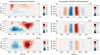 |
Fig. 1 One hundred-Earth-year mean streamfunction of oceanic meridional overturning circulation (MOC, left column) and atmospheric meridional circulation (right column) in the experiments with the default diffusivity (a− b), and 10 times(c−d) and 100 times (e−f) the defaultdiffusivity. The positive values represent the clockwise cells, and the negative values represent the anti-clockwise cells. The color bar in (e) is different from that in (a) and (c). |
3 Results
In this section, we answer the two questions introduced at the end of Sect. 1 by investigating the change of MOC and ocean heat transport with increased vertical diffusivity. We then describe the temperature change and the response of atmospheric circulation before discussing the three major feedback mechanisms that remarkably influence the global climate.
As shown in the left column of Fig. 1, when the diffusivity is 100*Kt0, the maximum value of the MOC increases from 18 to 324 Sv (1 Sv = 106 m3 s−1), with deep ocean overturning cells greatly strengthened. Here we utilize a simplified advective–diffusive balance to illustrate why the strength of MOC increases with greater vertical diffusivity. Consider a steady state with no source or sink of heat, the downward mixing of heat by diffusive processes below the thermocline is balanced by an upward advective heat flux, W∂z θ ≈ ∂z(Kt∂zθ), where W is the mean vertical velocity and θ is the potential temperature (Munk 1966; Vallis 2000; Wunsch & Ferrari 2004; Stewart 2008). If the ocean stratification does not change significantly with Kt (which is the case in our simulations; see Fig. 2), the MOC  approximately proportional to
  increases significantly with larger Kt. More complicated scaling analyses using the advective–diffusive balance, thermal wind relation, mass continuity, and thermodynamic equation suggest that the intensity of MOC is approximately proportional to
  or
or  (Welander 1971; Bryan 1987; Vallis 2000; Nikurashin & Vallis 2012). Our results are within these two ranges, with the MOC being about 3.3 (=100.52) and 18 (=1000.63) times the reference MOC in 10*Kt0 and 100*Kt0 cases, respectively (Table 1). As shown in Fig. 1a, the MOC of the modern Earth is pole-to-pole. When Kt is very large (Fig. 1e), all the deep water formed in the polar regions is brought up by the vertical mixing within its own hemisphere, and no Ekman suction is needed to bring up the water in the Southern Ocean as in the present day.
Due to the enhanced MOC, the peak of the meridional ocean heat transport increases from 1.82 to 4.25 PW (1 PW = 1015 W) (Fig. 3a). The ocean heat transport does not change proportionally with the MOC, because the MOC is substantially strengthened in the deep ocean, while the meridional ocean temperature gradient below the thermocline is much weaker than that of the surface ocean. This is consistent with previous studies of the vertical distribution of ocean heat transport on Earth: the shallow upper ocean circulation is more efficient in transporting heat because of the large temperature gradient there (Boccaletti et al. 2005; Saenko & Merryfield 2006; Ferrari & Ferreira 2011). Moreover, the latitude of the peak ocean heat transport shifts poleward by almost 20° in the 100*Kt0 case (Fig. 3a). When Kt is relatively small, the ocean heat transport peaks at low latitudes because both the vertical temperature gradient of the ocean (Fig. 4a) and the shallow meridional overturning driven by winds are large in the tropics. In the case of very large Kt, because of the substantial weakening of the wind-driven ocean circulation in the tropical and subtropical regions, and also the change in the structure of the MOC in the deep ocean (Figs. 1a,c,e), the peak of the ocean heat transport now appears at 30° latitude where the streamfunction is the largest (Fig. 1e).
In the simulations with 10*Kt0 and 100*Kt0, the planetary surface warms significantly (left column of Fig. 5), reaching a global-mean surface temperature of 4.2 °C and 9.5 °C above the reference temperature, respectively (Table 1). Figure 4e shows that the temperature of the deep ocean also increases significantly. With a large poleward ocean transport in the 100*Kt0 case, the temperature of polar ocean surface rises to 10–20 °C (Fig. 5e). As a result, the equator-to-pole surface temperature gradient reduces substantially. Moreover, given per unit energy, the change of surface temperature in the high latitudes is greater than that of the tropical regions, because the high-latitude surface is colder and loses less energy through thermal emission (the Planck effect, see Lohmann et al. 2016, Chap. 12), and this also decreases the equator-to-pole temperature gradient.
The atmospheric heat transport includes three components: sensible heat transport, latent heat transport, and geopotential energy transport. The effects of both mean flows and different types of waves (such as Rossby waves and large-scale gravity waves, but not subgrid-scale gravity waves) are included in the calculation of atmospheric heat transport. The meridional ocean heat transport only includes the dominant term, namely the advective heat transport ρCpvθ, where ρ is the seawater density, Cp is the specific heat capacity, v is the meridional velocity, and θ is the potential temperature. The predominant features of the atmospheric circulation response, including the tropical Hadley cells and the middle-latitude baroclinic eddies, become weaker with larger Kt (see the right column of Fig. 1) due to the decreased equator-to-pole temperature gradient. Consequently, the meridional heat transport carried by the atmosphere decreases (Fig. 3b), compensating the increase in ocean heat transport. Figure 3c shows clear compensation between atmospheric and oceanic heat transports, with total meridional heat transport increasing slightly with larger Kt in the northern hemisphere. The compensation in the meridional heat transport between atmosphere and ocean is a common feature in past, present, and future Earth climates, known as the Bjerknes compensation (e.g., Bjerknes 1964; Stone 1978; Yang et al. 2013a, 2016).
Above, we describe how the extremely large vertical mixing modifies the MOC, the surface temperature, and the atmospheric circulation. To better understand how the modified MOC influences the surface temperature, we investigated three essential feedback processes, including ice-albedo feedback, cloud feedback, and water vapor feedback (see Hartmann 2015, Chap. 10 and Lohmann et al. 2016, Chap. 12), as follows.
Global and one hundred-Earth-year mean characteristics of the simulated climate in three experiments with varying vertical diffusivity.
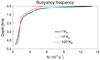 |
Fig. 2 Global and 100-Earth-year mean buoyancy frequency N |
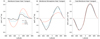 |
Fig. 3 One hundred-Earth-year mean meridional (south-to-north) ocean heat transport (OHT, a), atmospheric heat transport (AHT, b), and total heat transport (c) in three experiments. |
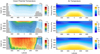 |
Fig. 4 One hundred-Earth-year and zonal mean ocean potential temperature (left) and air temperature (right) in the experiments with the default diffusivity (a− b), and 10 times(c−d) and 100 times (e−f) the default diffusivity. |
Ice-albedo feedback
The enhanced MOC transports more heat from the tropics to high latitudes (Fig. 3a), melting the sea ice there. The planetary surface is able to absorb more stellar energy because the surface albedo decreases (Table 1), which further melts the ice and snow in the polar regions. This positive ice-albedo feedback acts to substantially warm the surface and eventually melt all of the sea ice in the case with 100*Kt0 (Fig. 5f).
Cloud feedback
Fewer clouds form over the deep tropics with larger Kt (Figs. 6c, e, g), because the near-surface branches of the Hadley cells are weakened (right column in Fig. 1), leading to less convergence and weaker convection in the intertropical convergence zone. At middle latitudes, fewer baroclinic eddies result in fewer stratoculumus clouds and layered clouds (Hartmann 2015). At high latitudes, the clouds shift upward in altitude as the climate becomes warmer (Figs. 6c, e, g). Moreover, the cloud water concentration (the ratio of cloud water mass to total air or cloud mass), which is a measure of the liquid and ice water amount in the atmosphere, decreases with larger Kt (see Figs. 6d, f, h). The net result of these cloud responses is that the clouds become less reflective and the net cloud radiative effect (negative, a cooling effect) becomes smaller (Fig. 6a). For modern Earth, the simulated global-mean net cloud radiative effect is −27 W m−2, which is close to observations (see Hartmann 2015, Chap. 3). When the diffusivity is increased to 10 and 100 times the default value, the net cloud radiative effects are −23 W m−2 and −18 W m−2, respectively (Table 1). Therefore, the cloud feedback also has a warming effect on the planetary surface with larger Kt.
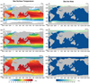 |
Fig. 5 One hundred-Earth-year sea surface temperature (left column) and sea ice fraction (right column) in the experiments with the default diffusivity (a−b), and 10 times(c−d) and 100 times (e−f) the default diffusivity. |
Water vapor feedback
When the atmosphere becomes warmer, more water vapor can be maintained in the atmosphere due to the Clausius-Clapeyron relation (e.g., Hartmann 2015, Chap. 1). As shown in Fig. 6b, the vertically integrated water vapor amount in the atmosphere increases greatly with larger Kt. Acting as an effective greenhouse gas, the increased water vapor further warms the planetary surface.
4 Summary and discussion
In this paper, we present three coupled global atmosphere-ocean numerical experiments that demonstrate the effect of varying vertical diffusivity on the climate of planets in the habitable zone. The main findings of this study are summarized in Fig. 7. Stronger tidal mixing intensifies MOC in the ocean, transporting more heat poleward. The enhanced ocean heat transport melts the polar sea ice and reduces the surface albedo, increasing the sea surface temperature. Other feedback processes associated with clouds and water vapor act to further warm the global surface. This study confirms a connection between planetary orbit, tidal mixing, ocean circulation, and planetary climate. The change of MOC due to larger vertical diffusivity could further influence the partition of CO2 between the atmosphere and ocean, as well as the spatial distributions of O2 and nutrients in the ocean.
The trend that we find, namely warming surface temperature with larger vertical diffusivity, and the responses of atmospheric circulation, clouds, and water vapor to increased oceanic heat transport are qualitatively consistent with previous studies of Earth’s climate in the past and future (Rind & Chandler 1991; Herweijer et al. 2005; Barreiro et al. 2011; Rose & Ferreira 2012; Koll & Abbot 2013; Knietzsch et al. 2015; Rencurrel & Rose 2018; Hilgenbrink & Hartmann 2018). However, in previous investigations, the change in vertical diffusivity was much smaller than that employed here and the magnitude of surface warming was also smaller.
The conclusion of this study is based on the simulations using Earth’s orbit and land–sea distribution. Further studies are required for planets with different continents. For Earth, strong tidal mixing is concentrated at the regions close to the ocean ridges(e.g., Waterhouse et al. 2014), and so the effect of tidal mixing on the planetary climate should also depend on the height, roughness, and spatial distribution of the topographic features of the seafloor. If the bottom of the ocean were flat, the tidal mixing would be weaker. Additionally, if the ocean were so deep that near-bottomocean mixing were not able to influence the upper ocean, the effect of tide-induced warming would also be smaller than that shown in this paper. The vertical diffusivity in this work is fixed in time and is assumed to be horizontally uniform. Future work is required to employ an ocean tide model (e.g., St. Laurent et al. 2002; Egbert et al. 2004; Green et al. 2019) to calculate the spatial pattern of the oceanic tides on different types of potentially habitable exoplanets, and to use high-resolution ocean general circulation models (e.g., Jansen 2016) to resolve the strength and spatial pattern of tidal mixing. The present computational speed and resources do not allow for this kind of simulation with a global-scale domain. Moreover, the effect of tidal heating, which can directly heat the ocean bottom (Mashayek et al. 2013), has not been considered in this work and should be included in the future.
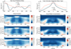 |
Fig. 6 One hundred-Earth-year and zonal mean net (shortwave plus longwave) cloud radiative effect at the top of the atmosphere (a), total (vertically integrated) water vapor amount in the atmosphere (b), cloud fraction (c, e, g), and cloud water concentration including liquid water and ice water (d, f, h) in three experiments with the default diffusivity (c−d), and 10 times(e−f) and 100 times (g−h) the default diffusivity. |
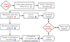 |
Fig. 7 Schematic showing how stronger tidal mixing leads to global surface warming. The stronger tidal mixing enhances the oceanic MOC and thereby the meridional ocean heat transport. As a result, the polar sea ice coverage decreases, and the ice-albedo feedback warms the surface. The stronger ocean heat transport also decreases the meridional temperature gradient and weakens the atmospheric convergence and baroclinic instability of the atmosphere, and the cloud feedback further warms the surface. In addition, water vapor feedback also acts to warm the planetary surface. |
Acknowledgements
J.Y. is supported by the National Natural Science Foundation of China under the grants 42075046 and 41888101. Y.S. acknowledges the scholarship provided by China Scholarship Council that supports her study at UCLA. The authorsthank Mingyu Yan for her help in preparing the manuscript. The authors sincerely appreciate the reviewer and editors for their insightful comments and suggestions, which have greatly improved the manuscript.
Appendix A Estimating the tidal mixing strength on potentially habitable planets around low-mass stars
In this Appendix, we roughly estimate the background vertical diffusivity Kt on potentially habitable planets around low-mass stars based on an analytic estimation of energy flux from ocean tides to internal waves (Bell 1975) and the equilibrium tide theory.
A.1 The energy flux from ocean tides to internal waves
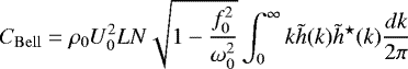
First, we introduce the energy flux from ocean tides to internal waves, which can be used to quantify the strength of ocean tidal mixing. Theoretically, this energy flux can be estimated as (Bell 1975; Smith & Young 2002):
 (A.1)
(A.1)
in units of Watts, where ρ0, U0, N, and f0 are the mean density of seawater, the amplitude of the barotropic tidal current, the buoyancy frequency, and the Coriolis frequency, respectively, ω0 is the fundamental tidal frequency, which we describe in Appendix A.3, L denotes the horizontal scale of the bottom topography,  is the Fourier transform of the topography, k is the wavenumber of the topography, and the star symbol denotes the complex conjugate. This equation is based on three assumptions: the fluid is unlimited in the vertical direction; the topography varies only in one direction; the buoyancy frequency is uniform in the ocean (Bell 1975; Smith & Young 2002; Nycander 2005). In the following sections, we provide our scalings of U0 and ω0 in order to estimate CBell and thus the background vertical diffusivity Kt on the potentially habitable exoplanets.
A.2 The maximum tidal height and barotropic tidal current amplitude
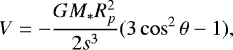
In this section, we estimate the tide-generating force and maximum tidal height, and then estimate the amplitude of the barotropic tidal current from the conversion between the potential energy and kinetic energy. In the equilibrium tide theory, the tide-generating potential is:
 (A.2)
(A.2)
where G is the gravitational constant, M* is the stellar mass,Rp is the planetary radius, s is the orbital distance, and θ is approximately equal to the zenith angle of the star (MacDonald 1964). The horizontal component of the tide-generating force is:
 (A.3)
(A.3)
The maximum tidal height (Kantha & Clayson 2000; Lv 2012) is expressed as:
 (A.4)
(A.4)
with the spherical triangle θ defined as
 (A.5)
(A.5)
where δ is the declination, φ0 is the latitude of the observer, and T1 is the hour angle. For an M dwarf–exoplanet system with a typical stellar mass M* = 0.3 Msun, typical orbital distance of planet in thehabitable zone s = 0.1 AU, Earth-like planetary radius Rp = REarth, and planetary mass Mp = MEarth, the horizontal tidal force F∥ and maximum tidal height ηmax are about 300 times those on Earth from the Sun (Eqs. A.3 and A.4), and 100 times those on Earth contributed by both the Sun and the Moon.
Tidal energy contains kinetic energy in tidal currents, and potential energy due to the rise and fallof water levels. During a tidal cycle, the maximum tidal potential energy is mgηmax, where m is the mass of seawater and g is the gravitational acceleration. The total kinetic energy of the tidal current can be scaled as the kinetic energy of the barotropic tides  , because most of the tidal energy comes from the barotropic tides (Carter et al. 2008), the velocity of which is vertically uniform. Assuming that all the tidal potential energy is eventually transferred into kinetic energy, the squared barotropic tidal current amplitude (
 ) is proportional to the maximum tidal height (ηmax). From the aforementioned discussion,
  in Eq. A.1 on such an exoplanet is about 100 times that on Earth.
A.3 The fundamental tidal frequency
In this section, we provide the method to scale ω0, the fundamental tidal frequency in Eq. A.1. Fundamental frequency refers to the lowest frequency of oscillatory flows, which is typically the frequency of external forcing. Waves are generated at the fundamental frequency, as well as at higher harmonics. In quasistatic fluid, the energy conversion from linear barotropic tides to internal waves is predominantly into the fundamental tidal frequency ω0 (Smith & Young 2002; Bell 1975). For barotropic tides,
 (A.6)
(A.6)
where  is the period of the maximum tidal height (e.g., Table 17.1 of Stewart 2008), and is the same as the period of the tide-generating potential (Doodson 1921; Stewart 2008). In Eq. A.5, the latitude of the observer φ0 is constant, and the declination δ changes very slowly over time. Therefore, the period of the spherical triangle θ is determined by the period of the hour angle T1, which is the least common multiple of Tr and To (denoted as lcm {Tr, To}) for slowly rotating planets. We therefore have ω0 ≈ 4π∕lcm{Tr, To}, based on Eqs. A.4, A.5, and A.6.
The Coriolis frequency at the latitude φ0 is
 (A.7)
(A.7)
where Tr is the rotation period of the planet. In middle latitudes where φ0 ≈ 1∕2, f0 ≈ 2π∕Tr.
Therefore, the term  in Eq. A.1 is approximately
  for a slowly rotating exoplanet. When
  , higher harmonics of tidal frequency (e.g., 2ω0, 3ω0,...) need to be considered. Here, we make a rough assumption that in Eq. A.1, the term
  is within the same order of magnitude as that of the present-day Earth. (For the present-day Earth–Moon system, the frequency of M2 tide is about two times the Coriolis frequency in middle latitudes, i.e.,
  .)
.)
A.4 Compare Kt and CBell on Earth and exoplanets
To estimate the magnitude of CBell on the asynchronously rotating planets around low-mass dwarfs, we assume that ρ0, L, and the integration related to the bottom topography in Eq. A.1 remain the same orders of magnitude as that on Earth. Based on the analysis and assumptions in sections A.2 and A.3, on such an exoplanet,  is around 100 times that on Earth, and
  does not change significantly for slowly rotating exoplanets. We further assume that in Eq. A.1 the buoyancy frequency on such an exoplanet is similar to that on Earth. In our experiments with varying background vertical diffusivities, the global mean buoyancy frequency remains within the same order of magnitude (Fig. 2).
Therefore, the energy flux from tides to internal waves on such an exoplanet is approximately 100 times that on Earth. With the assumption that there is a linear relation between Kt and CBell (Nycander 2005), the oceanic background vertical diffusivity Kt on rocky planets in the habitable zone of low-mass stars may be 100 times that on Earth.
This estimate has a lot of caveats because there are so many unknowns of exoplanets. It oversimplifies many factors that could make a difference to the scaling, such as bottom topography, spherical triangle, orbital period, rotation period, and different ocean stratification. A more accurate way to estimate the strength of tidal mixing is to employ a numerical tidal model such as that used in Green et al. (2019), but it would be much more expensive.
Appendix B Vertical profiles of background diffusivity
In this work, the key parameter is the background vertical thermal/salinity diffusivity in the ocean model. The K-Profile Parameterization (Large et al. 1994) is used to parameterize the unresolved vertical mixing. The background vertical thermal/salinity diffusivity (Kt) is
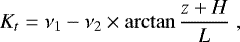 (B.1)
(B.1)
where ν1 = 5.24 × 10⁻⁵ m2 s−1 and ν2 = 3.13 × 10⁻⁵ m2 s−1 by default, z is the model vertical coordinate (z is positive upwards, and z = 0 for the mean sea level), H = 1000 m is the depth at which background vertical diffusivity is v1, L is the length scale where the transition in Kt takes place and 1∕L = 4.5 × 10⁻³ m−1 (Smith & Gent 2004). Figure B.1 shows the three vertical profiles of Kt employed in this study. The parameterizations of other types of mixing, including shear instability, convective instability, double diffusion, and boundary mixing, were not modified in any of the experiments.
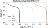 |
Fig. B.1 Profiles of the vertical thermal/salinity diffusivity Kt in the model CCSM3. The black line denotes default diffusivity Kt0, the blue line denotes 10 times the default diffusivity, and the red line denotes 100 times the default diffusivity. The ocean depth is the absolute value of z in Eq. B.1. |
References
- Auclair-Desrotour, P., Mathis, S., Laskar, J., & Leconte, J. 2018, A&A, 615, A23 [EDP Sciences] [Google Scholar]
- Barnes, R. 2017, Celest. Mech. Dyn. Astron., 129, 509 [Google Scholar]
- Barnes, R., & Deitrick, R. 2018, Handbook of Exoplanets (Berlin: Springer), 1 [Google Scholar]
- Barnes, R., Jackson, B., Greenberg, R., & Raymond, S. N. 2009, ApJ, 700, L30 [CrossRef] [Google Scholar]
- Barnes, R., Mullins, K., Goldblatt, C., et al. 2013, Astrobiology, 13, 225 [Google Scholar]
- Barreiro, M., Cherchi, A., & Masina, S. 2011, J. Clim., 24, 5015 [CrossRef] [Google Scholar]
- Bell, T. 1975, J. Fluid Mech., 67, 705 [NASA ADS] [CrossRef] [Google Scholar]
- Bjerknes, J. 1964, Adv. Geophys., 10, 1 [NASA ADS] [CrossRef] [Google Scholar]
- Boccaletti, G., Ferrari, R., Adcroft, A., Ferreira, D., & Marshall, J. 2005, Geophys. Res. Lett., 32, 10 [CrossRef] [Google Scholar]
- Briegleb, B., Bitz, C., Hunke, E., et al. 2004, Scientific description of the sea ice component in the Community Climate System Model, Technical Report, NCAR [Google Scholar]
- Bryan, F. 1987, J. Phys. Oceanogr., 17, 970 [NASA ADS] [CrossRef] [Google Scholar]
- Cael, B., & Ferrari, R. 2017, Geophys. Res. Lett., 44, 1886 [CrossRef] [Google Scholar]
- Carter, G. S., Merrifield, M., Becker, J. M., et al. 2008, J. Phys. Oceanogr., 38, 2205 [NASA ADS] [CrossRef] [Google Scholar]
- Checlair, J. H., Olson, S. L., Jansen, M. F., & Abbot, D. S. 2019, ApJ, 884, 1 [Google Scholar]
- Collins, W. D., Rasch, P. J., Boville, B. A., et al. 2004, Description of the NCAR community atmosphere model (CAM 3.0), Technical Report, NCAR [Google Scholar]
- Collins, W. D., Bitz, C. M., Blackmon, M. L., et al. 2006, J. Clim., 19, 2122 [CrossRef] [Google Scholar]
- Cullum, J., Stevens, D. P., & Joshi, M. M. 2016, Proc. Natl. Acad. Sci., 113, 4278 [NASA ADS] [CrossRef] [Google Scholar]
- Danabasoglu, G., Bates, S. C., Briegleb, B. P., et al. 2012, J. Clim., 25, 1361 [NASA ADS] [CrossRef] [Google Scholar]
- Del Genio, A. D., Way, M. J., Amundsen, D. S., et al. 2019, Astrobiology, 19, 99 [Google Scholar]
- Doodson, A. T. 1921, Proc. R. Soc. London Ser. A, 100, 305 [NASA ADS] [CrossRef] [Google Scholar]
- Driscoll, P., & Barnes, R. 2015, Astrobiology, 15, 739 [NASA ADS] [CrossRef] [Google Scholar]
- Egbert, G. D., Ray, R. D., & Bills, B. G. 2004, J. Geophys. Res. Oceans, 109, 1 [CrossRef] [Google Scholar]
- Ferrari, R., & Ferreira, D. 2011, Ocean Modell., 38, 171 [NASA ADS] [CrossRef] [Google Scholar]
- Gold, T., & Soter, S. 1969, Icarus, 11, 356 [NASA ADS] [CrossRef] [Google Scholar]
- Green, J. M., Way, M. J., & Barnes, R. 2019, ApJ, 876, L22 [NASA ADS] [CrossRef] [Google Scholar]
- Griffies, S. M. 2014, GFDL Ocean Group Technical Report No. 7, 1 [Google Scholar]
- Haqq-Misra, J., & Heller, R. 2018, MNRAS, 479, 3477 [NASA ADS] [CrossRef] [Google Scholar]
- Haqq-Misra, J., & Kopparapu, R. K. 2014, MNRAS, 446, 428 [Google Scholar]
- Hartmann, D. L. 2015, Global Physical Climatology (Amsterdam: Elsevier), 103 [Google Scholar]
- Heller, R., Leconte, J., & Barnes, R. 2011, A&A, 528, A27 [NASA ADS] [CrossRef] [EDP Sciences] [Google Scholar]
- Herweijer, C., Seager, R., Winton, M., & Clement, A. 2005, Tellus A Dyn. Meteorol. Oceanogr., 57, 662 [Google Scholar]
- Hilgenbrink, C. C., & Hartmann, D. L. 2018, J. Clim., 31, 9753 [NASA ADS] [CrossRef] [Google Scholar]
- Hu, Y., & Yang, J. 2014, Proc. Natl. Acad. Sci., 111, 629 [NASA ADS] [CrossRef] [Google Scholar]
- Ingersoll, A. P., & Dobrovolskis, A. R. 1978, Nature, 275, 37 [CrossRef] [Google Scholar]
- Jackson, B., Greenberg, R., & Barnes, R. 2008, ApJ, 681, 1631 [NASA ADS] [CrossRef] [Google Scholar]
- Jansen, M. F. 2016, J. Phys. Oceanogr., 46, 1917 [NASA ADS] [CrossRef] [Google Scholar]
- Jithin, A., Subeesh, M., Francis, P., & Ramakrishna, S. S. 2020, Sci. Rep., 10, 1 [NASA ADS] [CrossRef] [Google Scholar]
- Kantha, L. H., & Clayson, C. A. 2000, Numerical Models of Oceans and Oceanic Processes (Amsterdam: Elsevier), 66 [Google Scholar]
- Kasting, J. F., Whitmire, D. P., & Reynolds, R. T. 1993, Icarus, 101, 108 [Google Scholar]
- King, B., Stone, M., Zhang, H., et al. 2012, J. Geophys. Res. Oceans, 117, C4 [Google Scholar]
- Klymak, J. M., Legg, S. M., & Pinkel, R. 2010, J. Fluid Mech., 644, 321 [NASA ADS] [CrossRef] [Google Scholar]
- Knietzsch, M.-A., Schröder, A., Lucarini, V., & Lunkeit, F. 2015, Earth Syst. Dyn., 6, 591 [NASA ADS] [CrossRef] [Google Scholar]
- Koll, D. D., & Abbot, D. S. 2013, J. Clim., 26, 6742 [CrossRef] [Google Scholar]
- Lamb, K. G. 2014, Ann. Rev. Fluid Mech., 46, 231 [NASA ADS] [CrossRef] [Google Scholar]
- Large, W. G., McWilliams, J. C., & Doney, S. C. 1994, Rev. Geophys., 32, 363 [CrossRef] [Google Scholar]
- Leconte, J., Wu, H., Menou, K., & Murray, N. 2015, Science, 347, 632 [NASA ADS] [CrossRef] [Google Scholar]
- Lingam, M., & Loeb, A. 2018, Astrobiology, 18, 967 [NASA ADS] [CrossRef] [Google Scholar]
- Lohmann, U., Luond, F., & Fabian, M. 2016, An Introduction to Clouds: from the Microscale to Climate (Cambridge: Cambridge University Press), 399 [Google Scholar]
- Lv, H. 2012, Fundamentals of Physical Oceanography (China: China Ocean Press) [Google Scholar]
- MacDonald, G. J. 1964, Rev. Geophys., 2, 467 [NASA ADS] [CrossRef] [Google Scholar]
- MacKinnon, J. 2013, Nature, 501, 321 [NASA ADS] [CrossRef] [Google Scholar]
- Marshall, J., & Speer, K. 2012, Nat. Geosci., 5, 171 [NASA ADS] [CrossRef] [Google Scholar]
- Mashayek, A., Ferrari, R., Vettoretti, G., & Peltier, W. 2013, Geophys. Res. Lett., 40, 3144 [NASA ADS] [CrossRef] [Google Scholar]
- Munk, W. H. 1966, Deep Sea Res., 13, 707 [NASA ADS] [Google Scholar]
- Munk, W. H., & Wunsch, C. 1998, Deep Sea Res. Part I Oceanogr. Res. Papers, 45, 1977 [Google Scholar]
- Nikurashin, M., & Ferrari, R. 2013, Geophys. Res. Lett., 40, 3133 [NASA ADS] [CrossRef] [Google Scholar]
- Nikurashin, M., & Vallis, G. K. 2012, J. Phys. Oceanogr., 42, 1652 [NASA ADS] [CrossRef] [Google Scholar]
- Nycander, J. 2005, J. Geophys. Res. Oceans, 110, C10 [NASA ADS] [CrossRef] [Google Scholar]
- Oleson, K., Dai, Y., Bonan, B., et al. 2004, Technical description of the community land model (CLM), Technical Report, NCAR [Google Scholar]
- Olson, S. L., Jansen, M., & Abbot, D. S. 2020, ApJ, 895, 19 [NASA ADS] [CrossRef] [Google Scholar]
- Peters, H., Gregg, M. C., & Toole, J. M. 1988, J. Geophys. Res. Oceans, 93, 1199 [NASA ADS] [CrossRef] [Google Scholar]
- Rencurrel, M. C., & Rose, B. E. 2018, J. Clim., 31, 6299 [NASA ADS] [CrossRef] [Google Scholar]
- Rind, D., & Chandler, M. 1991, J. Geophys. Res. Atmos., 96, 7437 [NASA ADS] [CrossRef] [Google Scholar]
- Rose, B. E., & Ferreira, D. 2012, J. Clim., 26, 2117 [CrossRef] [Google Scholar]
- Saenko, O. A., & Merryfield, W. J. 2006, Geophys. Res. lett., 33, 6 [Google Scholar]
- Salehipour, H., Peltier, W., & Mashayek, A. 2015, J. Fluid Mech., 773, 178 [NASA ADS] [CrossRef] [Google Scholar]
- Schmittner, A., Green, J., & Wilmes, S.-B. 2015, Geophys. Res. Lett., 42, 4014 [NASA ADS] [CrossRef] [Google Scholar]
- Smith, R., & Gent, P. 2004, Reference Manual for the parallel ocean program (POP): ocean component of the community climate system model (CCSM2.0 and 3.0), Technical Report, NCAR [Google Scholar]
- Smith, S. G. L., & Young, W. R. 2002, J. Phys. Oceanogr., 32, 1554 [NASA ADS] [CrossRef] [Google Scholar]
- St. Laurent, L., Simmons, H., & Jayne, S. 2002, Geophys. Res. Lett., 29, 21 [Google Scholar]
- Stewart, R. H. 2008, Introduction to Physical Oceanography (USA: Texas A & M University) [Google Scholar]
- Stone, P. H. 1978, Dyn. Atm. Oceans, 2, 123 [NASA ADS] [CrossRef] [Google Scholar]
- Talley, L. D. 2011, Descriptive Physical Oceanography: an Introduction (Cambridge: Academic press) [Google Scholar]
- Vallis, G. K. 2000, J. Phys. Oceanogr., 30, 933 [NASA ADS] [CrossRef] [Google Scholar]
- Vallis, G. K. 2017, Atm. Oceanic Fluid Dyn. (Cambridge: Cambridge University Press) [CrossRef] [Google Scholar]
- Waterhouse, A. F., MacKinnon, J. A., Nash, J. D., et al. 2014, J. Phys. Oceanogr., 44, 1854 [NASA ADS] [CrossRef] [Google Scholar]
- Way, M. J., Del Genio, A. D., Aleinov, I., et al. 2018, ApJS, 239, 24 [NASA ADS] [CrossRef] [Google Scholar]
- Weber, T., & Thomas, M. 2017, Global Planet. Change, 158, 173 [Google Scholar]
- Welander, P. 1971, Phil. Trans. R. Soc. London, 270, 415 [CrossRef] [Google Scholar]
- Wilmes, S.-B., Schmittner, A., & Green, J. M. 2019, Paleoceanogr. Paleoclimatol., 34(8), 1437 [NASA ADS] [CrossRef] [Google Scholar]
- Wunsch, C., & Ferrari, R. 2004, Ann. Rev. Fluid Mech., 36, 281 [NASA ADS] [CrossRef] [Google Scholar]
- Yang, H., Wang, Y., & Liu, Z. 2013a, Tellus A, 65, 18480 [NASA ADS] [CrossRef] [Google Scholar]
- Yang, J., Cowan, N. B., & Abbot, D. S. 2013b, ApJ, 771, 771 [NASA ADS] [Google Scholar]
- Yang, J., Liu, Y., Hu, Y., & Abbot, D. S. 2014, ApJ, 796, L22 [CrossRef] [Google Scholar]
- Yang, H., Zhao, Y., & Liu, Z. 2016, J. Clim., 29, 2145 [CrossRef] [Google Scholar]
- Yang, J., Abbot, D. S., Koll, D. D., Hu, Y., & Showman, A. P. 2019a, ApJ, 871, 29 [NASA ADS] [CrossRef] [Google Scholar]
- Yang, J., Weiwen, J., & Yaoxuan, Z. 2020, Nat. Astron., 4, 58 [CrossRef] [Google Scholar]
- Zeng, Y., & Yang, J. 2021, ApJ, in press [Google Scholar]
Lee waves are internal gravity waves generated when large-scale quasi-steady ocean flows encounter relatively small-scale bathymetric features, such as sea mountains (e.g., Bell 1975). Figure 1 of MacKinnon (2013) is a nice visualization of lee waves in the ocean. The breaking of lee waves has been shown to be important for turbulent mixing at deep ocean (Nikurashin & Ferrari 2013; MacKinnon 2013).
The value of the Prandtl number ranges from slightly below 1 to about 10 for the ocean and is supposed to be dependent on the ocean state in terms of Renolds number and Richardson number (e.g., Salehipour et al. 2015). However, the turbulent Prandtl number is assumed to be a constant in most modern large-scale ocean models, although different values may be adopted in different models. For example, the Modular Ocean Model version 5 (MOM5, Griffies 2014) and the MIT General Circulation Model (MITgcm, Klymak et al. 2010) assume a turbulent Prandtl number of 1, while the Parallel Ocean Program (POP) assumes a value of 10 (Danabasoglu et al. 2012) based on field observations (Peters et al. 1988).
All Tables
Global and one hundred-Earth-year mean characteristics of the simulated climate in three experiments with varying vertical diffusivity.
All Figures
|
Fig. 1 One hundred-Earth-year mean streamfunction of oceanic meridional overturning circulation (MOC, left column) and atmospheric meridional circulation (right column) in the experiments with the default diffusivity (a− b), and 10 times(c−d) and 100 times (e−f) the defaultdiffusivity. The positive values represent the clockwise cells, and the negative values represent the anti-clockwise cells. The color bar in (e) is different from that in (a) and (c). |
| In the text | |
|
Fig. 2 Global and 100-Earth-year mean buoyancy frequency N |
| In the text | |
|
Fig. 3 One hundred-Earth-year mean meridional (south-to-north) ocean heat transport (OHT, a), atmospheric heat transport (AHT, b), and total heat transport (c) in three experiments. |
| In the text | |
|
Fig. 4 One hundred-Earth-year and zonal mean ocean potential temperature (left) and air temperature (right) in the experiments with the default diffusivity (a− b), and 10 times(c−d) and 100 times (e−f) the default diffusivity. |
| In the text | |
|
Fig. 5 One hundred-Earth-year sea surface temperature (left column) and sea ice fraction (right column) in the experiments with the default diffusivity (a−b), and 10 times(c−d) and 100 times (e−f) the default diffusivity. |
| In the text | |
|
Fig. 6 One hundred-Earth-year and zonal mean net (shortwave plus longwave) cloud radiative effect at the top of the atmosphere (a), total (vertically integrated) water vapor amount in the atmosphere (b), cloud fraction (c, e, g), and cloud water concentration including liquid water and ice water (d, f, h) in three experiments with the default diffusivity (c−d), and 10 times(e−f) and 100 times (g−h) the default diffusivity. |
| In the text | |
|
Fig. 7 Schematic showing how stronger tidal mixing leads to global surface warming. The stronger tidal mixing enhances the oceanic MOC and thereby the meridional ocean heat transport. As a result, the polar sea ice coverage decreases, and the ice-albedo feedback warms the surface. The stronger ocean heat transport also decreases the meridional temperature gradient and weakens the atmospheric convergence and baroclinic instability of the atmosphere, and the cloud feedback further warms the surface. In addition, water vapor feedback also acts to warm the planetary surface. |
| In the text | |
|
Fig. B.1 Profiles of the vertical thermal/salinity diffusivity Kt in the model CCSM3. The black line denotes default diffusivity Kt0, the blue line denotes 10 times the default diffusivity, and the red line denotes 100 times the default diffusivity. The ocean depth is the absolute value of z in Eq. B.1. |
| In the text | |
Current usage metrics show cumulative count of Article Views (full-text article views including HTML views, PDF and ePub downloads, according to the available data) and Abstracts Views on Vision4Press platform.
Data correspond to usage on the plateform after 2015. The current usage metrics is available 48-96 hours after online publication and is updated daily on week days.
Initial download of the metrics may take a while.