| Issue |
A&A
Volume 649, May 2021
|
|
|---|---|---|
| Article Number | A65 | |
| Number of page(s) | 10 | |
| Section | Cosmology (including clusters of galaxies) | |
| DOI | https://doi.org/10.1051/0004-6361/202140386 | |
| Published online | 13 May 2021 | |
Cosmography by orthogonalized logarithmic polynomials
1
Scuola Superiore Meridionale, Largo S. Marcellino 10, 80138 Napoli, Italy
e-mail: This email address is being protected from spambots. You need JavaScript enabled to view it.
2
Dipartimento di Fisica e Astronomia, Università degli Studi di Firenze, Via G. Sansone 1, 50019 Sesto Fiorentino, Firenze, Italy
3
Istituto Nazionale di Astrofisica (INAF) – Osservatorio Astrofisico di Arcetri, 50125 Florence, Italy
4
Dipartimento di Fisica “E. Pancini”, Università degli Studi di Napoli Federico II, Complesso Univ. Monte S. Angelo, Via Cinthia 9, 80126 Napoli, Italy
5
Istituto Nazionale di Fisica Nucleare (INFN), Sez. di Napoli, Complesso Univ. Monte S. Angelo, Via Cinthia 9, 80126 Napoli, Italy
6
Laboratory for Theoretical Cosmology, Tomsk State University of Control Systems and Radioelectronics (TUSUR), 634050 Tomsk, Russia
Received:
20
January
2021
Accepted:
15
February
2021
Abstract
Cosmography is a powerful tool for investigating the Universe kinematic and then for reconstructing the dynamics in a model-independent way. However, recent new measurements of supernovae Ia and quasars have populated the Hubble diagram up to high redshifts (z ∼ 7.5) and the application of the traditional cosmographic approach has become less straightforward due to the large redshifts implied. Here we investigate this issue through an expansion of the luminosity distance–redshift relation in terms of orthogonal logarithmic polynomials. In particular, we point out the advantages of a new procedure called orthogonalization, and we show that such an expansion provides a very good fit in the whole z = 0 ÷ 7.5 range to both real and mock data obtained assuming various cosmological models. Moreover, although the cosmographic series is tested well beyond its convergence radius, the parameters obtained expanding the luminosity distance–redshift relation for the Lambda cold dark matter (ΛCDM) model are broadly consistent with the results from a fit of mock data obtained with the same cosmological model. This provides a method for testing the reliability of a cosmographic function to study cosmological models at high redshifts, and it demonstrates that the logarithmic polynomial series can be used to test the consistency of the ΛCDM model with the current Hubble diagram of quasars and supernovae Ia. We confirm a strong tension (at > 4σ) between the concordance cosmological model and the Hubble diagram at z > 1.5. This tension is dominated by the contribution of quasars at z > 2 and also starts to be present in the few supernovae Ia observed at z > 1.
Key words: cosmology: theory / cosmological parameters / methods: analytical / methods: statistical / methods: observational
© ESO 2021
1. Introduction
The Universe is in a phase of accelerated expansion, as observed by cosmological probes such as local type Ia supernovae (SNe Ia; see e.g. Riess et al. 1998; Perlmutter et al. 1999) and the combination of SNe Ia, baryonic acoustic oscillations (BAOs), cosmic microwave background (CMB), and lensing provided by Planck Collaboration VI (2020). This acceleration is generally ascribed to the so-called dark energy. According to the concordance Lambda cold dark matter (ΛCDM) model, this dark energy component is naively associated with a cosmological constant (Λ) generated, in principle, by the quantum fluctuations of vacuum (Sahni & Starobinsky 2000; Carroll 2001; Peebles & Ratra 2003) and represents ∼70% of the total energy, being dominant in the current Universe. However, the huge discrepancy between the vacuum fluctuations of the primordial universe and the observed value of Λ today dramatically poses the so-called Cosmological Constant Problem (Weinberg 1989). The flat ΛCDM model is the one that, based on the simplest theory, can reproduce a large number of observations. Nevertheless, it suffers from both theoretical (e.g. fine-tuning and coincidence problems) and observational issues (e.g. the missing satellites problems; Bullock 2010). As a further example of the latter, we note the recent tension regarding the Hubble constant H0, which is the local value of the Hubble parameter H(z). The value of H0 inferred from the CMB, through the assumption of the flat ΛCDM model, is in tension at more than 4σ with the value measured from local sources (Cepheids, SNe Ia), as reported in Riess et al. (2019), and with that obtained in Wong et al. (2020) from lensed quasars. If we rule out systematic errors in these measurements, new physics beyond the standard cosmological model is needed (e.g. time-dependent dark energy equation of state, modified gravity, additional relativistic particles; see Capozziello et al. 2019a, 2020a; Dhawan et al. 2020; Alestas et al. 2021, 2020; Renzi & Silvestri 2020).
Model-independent approaches have been proposed to investigate the correct form of dark energy without any assumptions about its physical origin or the constituents of the Universe. Among these techniques, cosmography (Weinberg 1972) is one of the most consolidated. It relies only on the homogeneity and isotropy of the Universe without requiring any explicit physical function for the scale factor a(t), but only an analytical expression for it. The major problem of cosmography is that, to detect possible deviations from the standard cosmological model, data at high redshifts (i.e. z > 2) are necessary and convergence issues emerge in this redshift range (Capozziello et al. 2020b). If the data exceed the limit t ∼ t0 (z ∼ 0), where t0 is the present epoch, it is not correct to apply a Taylor expansion around t0, the one traditionally used in the cosmographic approach for the analytical approximation of a(t) (Visser 2004; Capozziello et al. 2019a). By definition of the Taylor expansion, this standard cosmographic approach gives an approximation of the luminosity distance DL(z), which is correct only around t = t0, in the limit of z ≤ 1. As a consequence, the cosmographic Taylor expansion cannot be used to analyse data at z ≥ 1. This was not a problem until recently as the only standard candles in the Hubble diagram were SNe observed up to z ∼ 1 (Betoule et al. 2014) for which the Taylor approach was completely justified. However, new SNe have been observed up to z = 2.26 by the Pantheon survey (Scolnic et al. 2018) and our research group has developed a method to turn quasars into standard candles (Risaliti & Lusso 2015, 2019; Salvestrini et al. 2019; Lusso & Risaliti 2016; Lusso et al. 2020) extending the Hubble diagram up to z ∼ 7.5 (Bañados et al. 2018). Thanks to this extended redshift range, the joint sample of quasars and SNe allows us to effectively look for discrepancies between the data and the standard cosmological model (see e.g. Rezaei et al. 2020), but this analysis would be possible only by solving the convergence issues described above. Some techniques have been recently proposed to alleviate this problem. In particular, using rational polynomials improves the convergence radius, which can then be used to approach higher redshift ranges, as in the case of the Padé and Chebyshev polynomials (see e.g. Aviles et al. 2014; Capozziello et al. 2018; Demianski et al. 2017; Zamora Munõz & Escamilla-Rivera 2020).
In this paper, we propose a novel technique. We try to overcome the weakness of cosmography at high redshifts by substituting the Taylor expansion with a new analytical function. We expand the luminosity distance in orthogonal polynomials of logarithmic functions. We investigate the advantages of this cosmographic technique in reproducing and testing cosmological models, and fitting the Hubble diagram of quasars and SNe. Once the robustness of the method has been proved, we also apply it to test the flat ΛCDM model.
The paper is structured as follows. In Sect. 2 we introduce the main features of cosmography, our logarithmic expansion and the “orthogonalization” procedure we are going to apply. Section 3 is focused on the basic demands of cosmography and on how the logarithmic expansion functions with them. This accurate analysis is also motivated by other cosmographic studies on the logarithmic approach (see e.g. Banerjee et al. 2020; Yang et al. 2020). The aim of this section is to demonstrate that, in the redshift range analysed in this work, our approach can be used to give a correct analytical reproduction of data and cosmological models and to test physical models. We then use this method as a cosmographic test of cosmological models in Sect. 4. In particular, we test the flat ΛCDM model through a joint fit1 of the Hubble diagram of quasars and SNe, confirming the tension with the flat ΛCDM at more than 4σ. Finally, in Sect. 5 we draw our conclusions, and present perspectives of our work. In Appendix A we explain how to properly perform the ortoghonalization procedure in the logarithmic function. In Appendix B we give the complete formulae for the fourth- and fifth-order logarithmic expansions in relation with a flat ΛCDM model.
Throughout the paper we use natural units with c = 1. Moreover, we assume a curvature k = 0 consistently with the most recent cosmological observations on CMB (Planck Collaboration VI 2020).
2. Cosmographic approach
The cosmographic approach is based only on the isotropy and homogeneity of the Universe through the assumption of the Friedmann-Lemaître-Robertson-Walker (FLRW) metric (Weinberg 1972). This is a purely geometrical description of the Universe kinematic in which all the physics is hidden in the scale factor a(t). A cosmographic approach does not depend on any cosmological assumption, except for the Cosmological Principle, as it does not require any equation of state of the cosmic fluid postulated a priori but only an analytical expression for the scale factor a(t) in the FLRW metric. This technique allows us to study the evolution of the Universe in a completely model-independent way.
In general, such an approach has two main advantages. First, if the adopted expansion is sufficiently flexible, it is able to fit the observational data with high accuracy, and second, the cosmographic parameters can be used to test any cosmological model (Capozziello et al. 2018; Escamilla-Rivera & Capozziello 2019). This is done by expanding the chosen cosmological model and the cosmographic series, which gives the relations between the physical parameters of the model and the cosmographic parameters (Aviles et al. 2014; Capozziello et al. 2019a; Benetti & Capozziello 2019). Then the values of these parameters are compared with the results of the cosmographic fit. An example of this approach is the fit of the Hubble diagram of SNe with a second-order Taylor expansion, whose free parameters are the Hubble constant H0 and the deceleration parameter q0 (Riess et al. 2004). The negative value of q0 obtained in this analysis provides the fundamental information on the present acceleration of the expansion of the Universe. Moreover, when q0 is expressed as a function of ΩM, 0 in a flat ΛCDM model, we obtain ΩM, 0 ∼ 0.3, and therefore ΩΛ, 0 ∼ 0.7. A further step in this approach is the inclusion of a third-order term in the cosmographic expansion, where the additional free parameter is called the “jerk” (Visser 2004) which is expected to be equal to 1 in a flat ΛCDM model. The fit of this third-order polynomial not only provides a more precise determination of q0, but it is also a test for the model itself: any significant deviation from 1 of the best-fit value of the jerk would be an indication of a tension between the data and the flat ΛCDM model (see e.g. Demianski et al. 2017).
In principle, this method can be used to test any cosmological model. However, as already stated in the previous section, in the past few years its application has become less straightforward due the increased redshift range of the observational data. This has introduced two new problems. First, the number of terms needed to reproduce the observational data with a cosmographic expansion has increased to four or even five (Demianski et al. 2017; Capozziello et al. 2020b; Benetti & Capozziello 2019), which makes the estimate of the significance of each parameter (and the comparison with the expectations of physical models) complicated due to the degeneracy among the cosmographic parameters. Second, even if the degeneracy issues are solved, it is not guaranteed that the results of a cosmographic fit can be compared with the theoretical prediction of a given physical model which is calculated around z = 0 (see e.g. Capozziello et al. 2019b).
The work we present in this paper is aimed at investigating and solving these two issues, in order to apply the cosmographic method to the complete Hubble diagram of SNe and quasars. In this section we introduce a cosmographic function consisting of orthogonal logarithmic polynomials, which solves the first problem. In Sect. 3, we discuss the second problem and validate our method in the whole z = 0 − 7.5 redshift range.
2.1. Cosmographic logarithmic approach and orthogonalization procedure
The cosmographic technique we propose is an extension of the one already described in some previous works (Risaliti & Lusso 2019; Lusso et al. 2019). It is based on an expansion of the luminosity distance as a power series of the quantity log10(1 + z). With respect to our previous works, we modified the expression of DL(z) to make the cosmographic coefficients orthogonal2. This makes our method unique: in the other cosmographic approaches all the coefficients are correlated as they are combinations of the ones at lower orders. The main advantage of the orthogonal polynomials is that a change in the truncation order of the series does not change the values of the cosmographic coefficients ai as they are uncorrelated. This allows us to test the significance of a possible additional term in the expansion (through its deviation from zero) and to evaluate the tension of the cosmographic fit with a given point in the parameter space without taking into account the correlation amongst free parameters.
We estimated the fifth-order for the orthogonal logarithmic polynomial expansion as3
![Mathematical equation: $$ \begin{aligned} D_{\rm L}(z)&= \frac{\mathrm{ln}(10)}{H_{0}} \Bigg \{ \mathrm{log}(1+z) + a_{2} \mathrm{log}^{2}(1+z) \nonumber \\&\quad + a_{3} \Bigg [ k_{32} \mathrm{log}^{2}(1+z) + \mathrm{log}^{3}(1+z)\Bigg ] \nonumber \\&\quad + a_{4} \Bigg [ k_{42} \mathrm{log}^{2}(1+z) + k_{43} \mathrm{log}^{3}(1+z) +\mathrm{log}^{4}(1+z) \Bigg ] \nonumber \\&\quad + a_{5} \Bigg [ k_{52} \mathrm{log}^{2}(1+z) + k_{53} \mathrm{log}^{3}(1+z) \nonumber \\&\quad + k_{54} \mathrm{log}^{4}(1+z) + \mathrm{log}^{5}(1+z) \Bigg ] \Bigg \} . \end{aligned} $$](/articles/aa/full_html/2021/05/aa40386-21/aa40386-21-eq1.gif) (1)
(1)
In our analysis, we tested the need for the different orders in this expansion proving the significance of the fifth-order (see Fig. 1 and the final comment of this section), while the sixth-order term turned out to be consistent with zero. This is the reason why we always consider an expansion to the fifth-order throughout the paper.
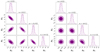 |
Fig. 1. Contour plots of the cosmographic free parameters ai for the non-orthogonal (left panel) and orthogonal (right panel) logarithmic fits to the fifth-order. Purple contours are the confidence levels at 1σ and 2σ. Best-fit values are very different in the two cases except for a5, which is consistent within the errors. This is expected from Eq. (1) as a5 is not multiplied by any factor kij and so must be equal to the same coefficient in the non-orthogonal formula. The apparent correlation in the (a3, a4) and (a4, a5) planes in the right panel is due to the prior DL > 0, which allows only specific values of ai. |
The terms  and a1 = 1 are needed to reproduce the Hubble law locally, that is
  . The coefficients kij in this formula are not free parameters, and depend on the data set we want to fit and, in particular, on its redshift distribution. They are determined through the step-by-step procedure described in detail in Appendix A. Nevertheless, our results are not affected by applying different sub-selections for the quasar sample. This is mainly because the quality filters employed in the selection of quasars produce a homogeneous sample of quasars (Lusso et al. 2020) and, as a consequence, a change in the final cleaned sample does not significantly modify the results even if the coefficients kij are formally sample dependent.
2.2. Data set and consequences of the orthogonalization procedure
Our data set consists of the sample of SNe from the Pantheon survey (Scolnic et al. 2018) and the sample of quasars described in Lusso et al. (2020) with the cutting at z > 0.7 (see Section 8 of the paper for an explanation of this selection filter). For a detailed description and validation of the procedure used to turn quasars into standard candles and for the fitting technique used to include them in the cosmological analysis, we refer to Risaliti & Lusso (2015, 2019), Salvestrini et al. (2019), Lusso & Risaliti (2016), and Lusso et al. (2020). Here we only point out that the non-linear relation between the X-ray and the UV emission of quasars used to turn them into standard candles depends on the luminosity distance, and so it requires the assumption of a specific cosmological model. We will discuss this point further when we explain the mocking procedure applied on quasars in Sect. 3.2.
Figure 1 shows the comparison between orthogonal and non-orthogonal4 cosmographic logarithmic fits to our data set (quasars + SNe). In the latter case, as we can see from the slanting contours (at 1σ and 2σ) in the parameter spaces of the left panel, the coefficients ai are correlated. As a consequence, a change in the order of the polynomial would modify the best-fit values of the parameters. We can see this directly by comparing the non-orthogonal fourth-order fit shown in Fig. 2 to the fifth-order fit in Fig. 1. Instead, in the case of the orthogonal polynomial (right panel of Fig. 1) there is no covariance at all between the parameters.
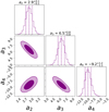 |
Fig. 2. Same as Fig. 1, but for the fourth-order non-orthogonal fit. The best-fit values of ai are different from those of the fifth-order non-orthogonal fit shown in Fig. 1, which is a consequence of the correlation between the parameters. These values are also inconsistent with those of the fifth-order orthogonal fit, except for a4 (as already explained for a5; see Fig. 1). |
As anticipated, the results of the fits in Fig. 1 show that the fifth-order is significant, with a deviation from zero of about 3σ, and so it is required to fit our set of data.
3. Validation of the cosmographic logarithmic approach
The cosmographic function is fitted over a redshift range much broader than the convergence radius of the logarithmic expansion. Therefore, we need to check if this expansion is still useful for testing physical models. We note that in this paper we are only interested in the validation of the cosmographic approach within the redshift range of the observational data, while we do not discuss the extrapolation of the model to higher redshifts or the related convergence issues.
In order to compare a cosmographic fit with the predictions of a physical model, we use the relations that hold between the cosmographic and physical free parameters, as described in Sect. 2. However, this technique is strictly valid only in a redshift range up to z ∼ 1 (due to the expansions centred in z = 0). The comparison with a fit on the whole redshift range may not be strictly correct. Nevertheless, it could be possible that the cosmographic expansion represents a good approximation even if the redshift range goes beyond the convergence radius just because its shape is similar to that of the cosmological model.
We investigated this issue in two ways: first we compared the cosmographic expansion of the flat ΛCDM model with the model itself for different values of ΩM, 0 (Sect. 3.1), then we compared the predictions of the cosmographic expansion with the fits of mock samples in the z = 0 − 7.5 range (Sect. 3.2).
3.1. Cosmographic expansion of physical models
In order to check whether the cosmographic logarithmic expansion is a good approximation of the ΛCDM model beyond the convergence radius, we analysed the ratio of the physical model to its logarithmic expansion, as a function of the redshift. The results are shown in Fig. 3 (which reproduces Fig. 1c of Banerjee et al. 2020). The parameter R represents the ratio of the luminosity distance estimated from the fifth-order cosmographic approximation of a specific flat ΛCDM model with H0 = 70 km s−1 Mpc−1 and five different choices of ΩM, 0 (ΩM, 0 = 0.1, 0.28, 0.5, 0.7, 0.9) to the luminosity distance from the corresponding cosmological model. The numerator of R is obtained using the relations between ai and ΩM, 0 calculated through the expansions in z = 0, as described above. These relations depend on the truncation order of the expansion and on the sample, due to the presence of the coefficients kij. We refer to Appendix B for the exact expressions of ai (ΩM, 0) in a logarithmic expansion at fourth- and fifth-order. The redshift range we considered in Fig. 3 corresponds to that spanned by our data, up to z ≃ 7.5.
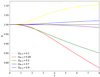 |
Fig. 3. Luminosity distance ratio (R) of a fifth-order cosmographic expansion of a flat ΛCDM model to the model itself, for different values of ΩM, 0. In each case the expansion very precisely reproduces the cosmological model for z < 1 (R = 1). The discrepancy from R = 1 at z > 1 depends on the specific value of ΩM, 0: the worst case is for ΩM, 0 = 0.28, while the best case is for ΩM, 0 = 0.9. |
From this analysis we conclude that in all the cases the cosmological model is well reproduced up to z ∼ 1. This implies that it is correct to compare the best-fit values of the cosmographic free parameters and the prediction of the cosmological model for these parameters only for fits at z ≤ 1. Moreover, the logarithmic expansion always shows a limited deviation from the ΛCDM model within the whole redshift range: the larger discrepancy from R = 1 is ∼0.2 at the maximum redshift z ∼ 7.5 for the case with ΩM, 0 = 0.28, which corresponds to a relative difference in distance modulus of 0.01. This implies that the logarithmic approximations and the reference cosmological models have the same shapes, that is to say the same trend with redshift.
3.2. Comparison with fits of mock samples
A direct way to check the applicability of a cosmographic analysis on a wide redshift range is through mock samples of data. Thanks to this procedure we can simulate sets of data that have the same redshift distribution, statistical errors, and intrinsic dispersion in distance modulus as the real sample and that follow a specific cosmological model. This sample is very different from the ideal one used in Fig. 3 where statistical errors and dispersion are not taken into account and where we have assumed an almost continuous distribution in redshift. As a consequence, a mock sample can be used to fit the cosmographic model on a real set of data that assumes a specific cosmological model, and this fit can be compared with the theoretical prediction obtained by the analytical expansion around z = 0. This approach allows to turn the qualitative comparison between DL(z) (as in Fig. 3) into a quantitatively comparison in the ai bi-dimensional spaces. This is the crucial test to investigate whether the prediction from an expansion at z = 0 can be extrapolated up to redshifts z ∼ 8.
We now explain in detail the procedure we followed starting from the creation of the mock samples of quasars and SNe. Regarding SNe, we calculated the mock distance moduli5 using the redshifts from the Pantheon sample and DL(z) from a flat ΛCDM model (DM(z) = 5 log(DL(z)(Mpc)) + 25) with H0 = 70 km s−1 Mpc−1 and two values of ΩM, 0: ΩM, 0 = 0.28 and ΩM, 0 = 0.7. We also included in the calculation of the distance moduli the contribution of a Gaussian distribution with an intrinsic dispersion around the central value of 0.16 dex. The statistical errors associated with the distance moduli are those from the real sample. The mock samples of quasars have the same redshifts and UV luminosity as the real set of data (Lusso et al. 2020) and X-ray fluxes obtained from the X-UV relation under the assumption of a flat ΛCDM model with the same values of H0 and ΩM, 0 assumed for the mock samples of SNe. As for SNe, we also took into account their intrinsic dispersion. Specifically, we assumed a Gaussian distribution in the distance modulus around 1.3 dex. Once again the statistical errors on the distance moduli are those from the real sample of data. The number of sources in these mock samples is increased (for both quasars and SNe) in order to constrain the free parameters of the fits with higher precision, leaving the relative statistical weight of quasars and SNe unchanged. For every redshift we generated 100 sources with slightly different distance moduli due to the Gaussian distribution of the intrinsic dispersion. Thanks to this, we improved the precision on the best fit of the free parameters by a factor 10 making the uncertainties negligible compared to those of the real data6.
Following this method we built two joint mock samples of quasars and SNe assuming ΩM, 0 = 0.28 and ΩM, 0 = 0.7, respectively. These choices are justified by the fact that, looking at Fig. 3, these are the cases in which the cosmological model is worst and best (just after ΩM, 0 = 0.9) reproduced by the expansion around z = 0, respectively. The conclusions we obtain for these two extreme cases can be generalized to all the other intermediate cases. Moreover, ΩM, 0 = 0.28 is the value actually favoured by several cosmological probes, and so it is of common interest to test our method on this specific value.
As a self-consistency check, we first recover the cosmological parameters through a direct fit of a flat ΛCDM model to the mock data. The inferred best-fit values of ΩM, 0 and H0 are shown in Table 1. This test quantifies the degree of randomness introduced in the mocking procedure and confirms that the data are fully consistent with the specific flat ΛCDM model assumed.
Best-fit values of ΩM, 0 and H0 from the mock samples of data built according to the correspondent cosmological models.
The mock samples of quasars and SNe obtained in this way are fitted jointly with a fifth-order orthogonal logarithmic function. We study the two cases of ΩM, 0 = 0.28 and ΩM, 0 = 0.7 separately finding, in the end, some generalized conclusions.
Figure 4 summarizes the results for the case with ΩM, 0 = 0.28. Each panel in this figure shows a bi-dimensional free parameter space of ai in which the confidence levels from 1σ to 4σ refer to the cosmographic analysis on the real set of data of quasars from Lusso et al. (2020) and SNe from the Pantheon survey (and are exactly the ones already shown on the right side of Fig. 1), the red point is the best fit from the mock sample, while the green star is the analytic prediction from the expansion of the standard model around z = 0 (Eq. (B.2) for ΩM, 0 = 0.28).
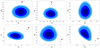 |
Fig. 4. Bi-dimensional spaces for the cosmographic free parameters ai. In each panel, the blue contours are the confidence levels at 1σ, 2σ, 3σ, and 4σ for the best fit on the real set of data (quasars+SNe), the red point is the best fit from the mock sample with ΩM, 0 = 0.28 and the green star corresponds to the prediction of the corresponding ΛCDM model from the expansion in z = 0. |
Focusing on the comparison between the red point and the green star, we see that they perfectly match on the parameter a2, while the green star underestimates the discrepancy from observational data of 0.7σ in a3 and 1.5σ in a4 and overestimates the same discrepancy of 1σ in a5. This means that the prediction in the limit z < 1 is in good agreement with the correct results also when evaluated over the whole redshift range. Furthermore, this analysis shows something more interesting under a deeper insight. The discrepancy between the data and the ΛCDM model with ΩM, 0 = 0.28 (green star) is at more than 6σ and 7σ for a3 and a4, respectively. Moreover, for these two parameters, the prediction of the expansion at z = 0 (green star) affects the results with an underestimation of the discrepancy if compared to the fit on the mock sample (red point). As a consequence, the claim for the existence of a tension coming from the comparison between data and analytic prediction would be correct and confirmed at even more sigmas by the use of mock samples. The results on the parameter a5, instead, require a more complex interpretation. In this case, the discrepancy of the data with the red point (the best fit from the mock sample) and the green star (the prediction from the expansion) is at 2.7σ and 3.8σ, respectively. Nevertheless, we need to consider that a5 is the less significant parameter, and that it is less constrained because of the high errors. So, if a larger sample of quasars at high redshifts (where this term is dominant) were available, we expect that a5 could be constrained better leading to a much more significant discrepancy from the cosmological model, such as those observed in a3 and a4. If this happens the argument on a3 and a4 could also be generalized to this parameter. From this last point it is evident that future observations of quasars at high redshifts could play a crucial role, which could certainly make this analysis easier and clearer.
The complexity of this analysis and the care needed to take every aspects into account lead us, in the end, to demonstrate the great advantages of the logarithmic approach. On the one hand, the fifth-order orthogonal logarithmic function can precisely reproduce the given physical model, as proved by the fit on the mock data. On the other hand, as we are only interested in comparing the data with cosmological models to test for a possible tension, we can directly compare the fit in the whole redshift range with the prediction from the expansion at z = 0 without the need of mock samples as the approximation introduced with this method is negligible.
We demonstrated it for ΩM, 0 = 0.28, but as already pointed out this is the case in which the analytic prediction has the maximum deviation from the model (Fig. 3), and so these conclusions can be generalized to all the other flat ΛCDM models with values of ΩM, 0 between 0.1 and 0.9. Moreover, in all the other cases we expect a better agreement of the theoretical prediction and a solid confirmation of the results described above.
As an example of this statement, we show in Fig. 5 the same analysis for a flat ΛCDM model with ΩM, 0 = 0.7. The key result is that the green star and the red point completely overlap in each of the parameter spaces leading to a perfect match between the physical model and the prediction at z = 0.
This is strong evidence that the cosmographic extrapolation can be used at redshifts z > 1. This allows us to avoid fitting mock samples for every possible value of ΩM, 0 to reproduce the curve predicted by a flat ΛCDM model in the parameter spaces substituting this long-time computational procedure with the simple analytic calculation at z ∼ 0.
Summarizing, we have studied in detail the features of our cosmographic approach showing that the logarithmic function has excellent properties and can reproduce physical models over the whole redshift range of the data considered. As a consequence, we can use this method to describe the Hubble diagram of quasars and SNe analytically, and to compare it with the predictions of cosmological models.
The method we have just described is completely general and can be applied to any cosmographic function to test whether its theoretical prediction at z = 0 can be compared to the cosmographic fit over the whole redshift range. This gives us an unbiased measure of the usefulness and the power of different cosmographic approaches.
4. Test of the flat ΛCDM model
Once we have demonstrated the robustness of the cosmographic logarithmic technique, the next step is to use it as a test for cosmological models. We have proved that our cosmographic function gives a reliable reproduction of a flat ΛCDM model if we assume this model as the reference one, but we can also compare the prediction of the standard cosmological model with the observational data taking advantage of the degrees of freedom and the flexibility of the logarithmic function. This means fitting the data with both cosmological and cosmographic models with the purpose of studying the following: (1) the deviations of the distance moduli; (2) the different trends of the two best-fit curves in the Hubble diagram; and (3) the discrepancy between the best-fit values of ai and the values of ai predicted by the cosmological model. Regarding this last point, we have already shown (see previous section) that it is correct to compare the findings obtained with the data over the whole redshift range with the theoretically predicted values of ai(ΩM, 0) obtained by the expansion around z = 0.
An analysis of this kind is possible only because we have defined a model that has good convergence properties and that guarantees a purely analytical reconstruction of the data as it does not rely on any physical assumptions on the evolution of the Universe or on the nature of its constituents (except for the assumption of the FLRW metric). In principle, this cosmographic model can be used as a test for any cosmological model, but in this paper, we focus only on a flat ΛCDM model, while the study of other cosmological models will be developed in forthcoming dedicated publications.
As the first step we fitted the distance moduli of the joint sample of quasars (Lusso et al. 2020) and SNe Ia (Scolnic et al. 2018) with the cosmographic logarithmic orthogonal expansion to the fifth-order (Eq. (1) with the coefficients kij fixed for this sample through the procedure described in Appendix A) and with a flat ΛCDM model. The fit of the flat ΛCDM model is performed not only on the whole redshift range of the data, but also in the restricted interval with z < 1.1, where SNe are predominant, to get a deeper insight into the comparison between this cosmological model and the observational data.
In Fig. 6, we plot the redshift-averaged sigma deviations between the cosmographic distance moduli of quasars (yellow bars) and SNe (blue bars) and the best-fit ΛCDM model up to z = 1.1 and extrapolated to higher redshifts. The discrepancy between the ΛCDM model and the data is clearly due to a deviation from the Hubble diagram of quasars at z > 1. This tension increases with redshift, reaching a peak at z = 2 − 3 and remaining statistically significant up to the highest redshifts. This is a step forward from the results presented in Lusso et al. (2019) where the same discrepancy reaches a peak at z ∼ 3, the redshift of high-quality pointed observations, but it almost vanishes at z > 3 where the data quality is lower (see their Fig. 5). The authors already suggested that observations of quasars at z ∼ 4 were required to verify this trend. In our sample of quasars new observations at z > 4 have been included with a tension that is still high at these redshifts, confirming the discrepancy at high redshifts. As a final comment, it should be noted that quasars are not the only objects responsible for this discrepancy. In fact, SNe at z > 1 (∼23 SNe) already display the same trend and the same evidence of a deviation. As SNe are the most powerful and reliable standard candles in the cosmological analysis, this is a very strong piece of evidence for the existence of a tension between the ΛCDM model and the observations. These results, already mentioned in Risaliti & Lusso (2019) and Lusso et al. (2019), are now confirmed with greater statistical significance thanks to our new sample of quasars.
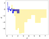 |
Fig. 6. Deviations (in unity of σ) of the cosmographic distance moduli of quasars (yellow bars) and SNe (blue bars) from the best-fit ΛCDM model up to z = 1.1 and extrapolated to higher redshifts. The values of σ are redshift-averaged in narrow logarithmic bins. A discrepancy between the data and the model emerges at z ≥ 1 and it remains significant at higher redshifts. This proves the tension between the ΛCDM model and the observations. |
These considerations are reinforced if we analyse the fit of the ΛCDM model on the whole redshift range. In Fig. 7 we show the Hubble diagram of quasars (yellow points) and SNe (cyan points) and the best-fit curves of the logarithmic function (continuous black line) and the flat ΛCDM model (dashed magenta line) over the whole range of z. As the fitting technique requires both the marginalization over all free parameters and the sigma-clipping procedure7 on the quasar sample (see Lusso et al. 2020 for more details), we decided to plot the values of the distance moduli computed through the cosmographic fit. The points corresponding to the ΛCDM best-fit model would be different in terms of the number of quasars (due to the sigma-clipping) and the distance moduli (due to the marginalization), but this difference is very small and graphically not significant. There are only four more quasars, not removed by the sigma-clipping, in the sample produced by the best-fit ΛCDM model; the mean value of the difference between the distance moduli (DMΛCDM − DMlog) is ∼0.3 with an absolute maximum difference of about 1.3 at z ∼ 3. This is the reason why, for visual clarity, we have decided to plot both the best-fit curves on the same Hubble diagram (that from the cosmographic fit), even if this is not formally correct.
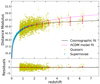 |
Fig. 7. Top panel: hubble diagram of SNe (cyan points) and quasars (yellow points). The red points are averages (along with their uncertainties) of the distance moduli of quasars in narrow (logarithmic) redshift intervals and they are shown for visualization purposes only, without any statistical application. Dashed magenta and continuous black lines show respectively the best-fit curves of the flat ΛCDM and the logarithmic models over the whole redshift range. Bottom panel: residuals with respect to the cosmographic fit for quasars and averages of the residuals over the same redshift intervals. |
The main difference from the previous analysis is that the ΛCDM model is fitted over the entire redshift range. Compared with the analysis on the data at z < 1.1 we note that the best-fit values of ΩM, 0 are consistent within the error bars (ΩM, 0 = 0.281 ± 0.013 for z < 1.1 and ΩM, 0 = 0.296 ± 0.013 over the whole range of z) and the best-fit curves on the Hubble diagram are indistinguishable with a maximum absolute difference in distance modulus of 0.04.
The best-fit curves of the cosmological and cosmographic models shown in Fig. 7 are completely overlapping in the low-redshift region at z < 1, whilst the tension becomes significant at z > 1.5, where the prediction of the ΛCDM model is much steeper than that of cosmography.
To quantify the discrepancy between these two curves we can compare the best-fit values of ai from the cosmographic fit with those predicted from the ΛCDM model (see Appendix B, relations B.2). This comparison is exactly the one between the blue contours and the green star8 already shown in Fig. 4 for the concordance model (ΩM, 0 = 0.28) and in Fig. 5 for the case with ΩM, 0 = 0.7. Focusing on the concordance model (Fig. 4), as it is the most accepted and successful one, we note that there is no tension on a2, the dominant term at low redshifts. This is further evidence of the agreement between the ΛCDM model and the data up to z ∼ 1 already shown in the analysis above. Nevertheless, due to the increasing discrepancy on the other parameters and so at higher redshifts, the overall tension between the cosmographic fit and the cosmological model is much greater than 4σ. This confirms the results of Risaliti & Lusso (2019) and Lusso et al. (2019) with evidence of an increased discrepancy between the standard cosmological model and the data.
5. Conclusions
We critically analysed the role of cosmography and its potential issues focusing on the problems that emerge when observational data go beyond z ∼ 1. We also discussed the possibility to reproduce and fit the data and the standard cosmological model with the final aim of developing a completely model-independent technique to test any cosmological models. Here we presented a new cosmographic technique based on a polynomial logarithmic function.
Firstly, we showed that the new orthogonalization procedure allows us to quantify the discrepancy between the cosmographic fit and any given point in the free parameter spaces without taking into account the possible correlation amongst the free parameters. Moreover, we proved that a fifth-order in the logarithmic polynomial is needed to fit data up to the maximum redshifts of quasars (z ∼ 7.5), while a sixth-order would not be significant. Then, we studied the behaviour of the logarithmic function in the local range z ∼ 0 through an expansion centred at z = 0, and we checked for the possibility to compare this cosmographic function with the prediction of a flat ΛCDM model in the same redshift range. The main result was that this expansion is convergent and correctly reconstructs the model. As a consequence, it can be used to fit data and test cosmological models if we set a limit of z ≤ 1. After that, we extended this study to the highest redshifts observed (z ∼ 7.5) through the use of mock samples as we are not interested in the asymptotic limit where data are not currently available. This analysis showed that an extrapolation to z > 1 of the logarithmic polynomial with coefficients obtained by the expansion at z = 0 is robust if we are only interested in a possible tension between the data and the flat ΛCDM model. The precision of the cosmographic prediction in the redshift interval z = 1 − 7.5 depends on the value of ΩM, 0 considered, but it always allows a direct comparison between the cosmographic fit and the prediction of flat ΛCDM models with any physical values of ΩM, 0. Summarizing this first part of the work, for a cosmographic analysis of the Hubble diagram of quasars and SNe we need to use the orthogonal logarithmic approach to obtain a reliable reconstruction of data at z > 1 that can be compared with the predictions of cosmological models.
In the second part of the work we fitted the Hubble diagram of quasars and SNe with a fifth-order orthogonal logarithmic function and a flat ΛCDM model. The main results are the following:
-
the Hubble diagram is well reproduced by the ΛCDM model up to z ∼ 1;
-
a discrepancy emerges at higher redshifts mainly due to quasars, but also due to SNe at z > 1, even if with less statistical significance, and it increases with redshift;
-
the overall tension between cosmographic and cosmological fits is greater than 4σ.
In conclusion, we proved that the orthogonalized logarithmic approach we developed is a powerful and reliable tool that reproduces analytically the Hubble diagram of quasars and SNe at least up to z ∼ 7.5 and that tests the predictions of cosmological models.
As we have already pointed out, this work is mainly methodological and it opens the way to analyse the suitability of other cosmographic approaches. In a forthcoming paper we will apply the method developed to some Padè polynomials (see Benetti & Capozziello 2019 and Capozziello et al. 2020b). In this case it would also be possible to include a study on the convergence features of these series at high redshifts, while the convergence of our logarithmic function was already expected due to the logarithmic shape.
Moreover, in this paper we only considered a flat ΛCDM model as a first application of the orthogonalized cosmographic logarithmic technique. Future works will focus on testing other cosmological models, especially those with an evolving dark energy contribution and with a possible interaction between dark energy and dark matter (i.e. interacting dark energy models) or models coming from modified gravity (Capozziello et al. 2019a).
A further step would be to extend the sample used in the cosmological analysis (only quasars and SNe) including other cosmological probes (e.g. CMB, BAO) to study the relationship between early- and late-time Universe dynamics in the framework of a specific cosmological model.
The fits presented in this work were all obtained by employing a fully Bayesian Markov chain Monte Carlo (MCMC) approach. Specifically, we considered the affine-invariance MCMC Python package emcee (Foreman-Mackey et al. 2013), where the estimated uncertainties on the parameters are taken into account. This technique has already been adopted in Capozziello et al. (2011).
Through this paper we use the term “orthogonal” to mean “with no covariance”.
For sake of simplicity we use log instead of log10 and ln instead of loge.
The formula for DL in the fifth-order non-orthogonal case is simply
![Mathematical equation: $$ \begin{aligned} D_{\rm L}(z)=&\frac{\mathrm{ln}(10)}{H_{0}} \Bigg [\mathrm{log}(1+z) + a_{2} \mathrm{log}^{2}(1+z)\nonumber \\&+ a_{3}\mathrm{log}^{3}(1+z)+ a_{4}\mathrm{log}^{4}(1+z)+ a_{5} \mathrm{log}^{5}(1+z) \Bigg ].\end{aligned} $$](/articles/aa/full_html/2021/05/aa40386-21/aa40386-21-eq6.gif) (2)
(2)
Throughout the paper the abbreviation “DM” used in equations stands for the distance modulus and not for the dark matter component.
This is a method commonly used to remove possible outliers in the data set. Specifically, it consists of discarding every source that has a discrepancy of more than a specific number of σ (in our case 3σ) from the best-fit model. The iteration of this procedure guarantees a better estimation of the free parameters of the model.
As proved in Sect. 3.2, we are allowed to use the green star instead of the red point as the reference for the prediction of the cosmological model.
References
- Alestas, G., Kazantzidis, L., & Perivolaropoulos, L. 2020, Phys. Rev. D, 101, 3516 [Google Scholar]
- Alestas, G., Kazantzidis, L., & Perivolaropoulos, L. 2021, Phys. Rev. D, 103, 3517 [Google Scholar]
- Aviles, A., Bravetti, A., Capozziello, S., & Luongo, O. 2014, Phys. Rev. D, 90, 043531 [NASA ADS] [CrossRef] [Google Scholar]
- Bañados, E., Venemans, B. P., Mazzucchelli, C., et al. 2018, Nature, 553, 473 [NASA ADS] [CrossRef] [Google Scholar]
- Banerjee, A., Colgáin, E., Sasaki, M., Sheikh-Jabbari, M. M., & Yang, T. 2020, ArXiv e-prints [arXiv:2009.04109] [Google Scholar]
- Benetti, M., & Capozziello, S. 2019, JCAP, 1912, 008 [Google Scholar]
- Betoule, M., Kessler, R., Guy, J., et al. 2014, A&A, 568, A22 [NASA ADS] [CrossRef] [EDP Sciences] [Google Scholar]
- Bullock, J. S. 2010, ArXiv e-prints [arXiv:1009.4505] [Google Scholar]
- Capozziello, S., Lazkoz, R., & Salzano, V. 2011, Phys. Rev. D, 84, 124061 [NASA ADS] [CrossRef] [Google Scholar]
- Capozziello, S., D’Agostino, R., & Luongo, O. 2018, MNRAS, 476, 3924 [CrossRef] [Google Scholar]
- Capozziello, S., D’Agostino, R., & Luongo, O. 2019a, Int. J. Mod. Phys. D, 28, 1930016 [CrossRef] [Google Scholar]
- Capozziello, S., Ruchika, S., & Sen, A. A. 2019b, MNRAS, 484, 4484 [NASA ADS] [CrossRef] [Google Scholar]
- Capozziello, S., Benetti, M., & Spallicci, A. D. A. M. 2020a, Found. Phys., 50, 893 [NASA ADS] [CrossRef] [Google Scholar]
- Capozziello, S., D’Agostino, R., & Luongo, O. 2020b, MNRAS, 494, 2576 [CrossRef] [Google Scholar]
- Carroll, S. M. 2001, Liv. Rev. Relativ., 4, 1 [Google Scholar]
- Demianski, M., Piedipalumbo, E., Sawant, D., & Amati, L. 2017, A&A, 598, A113 [CrossRef] [EDP Sciences] [Google Scholar]
- Dhawan, S., Brout, D., Scolnic, D., et al. 2020, ApJ, 894, 54 [Google Scholar]
- Escamilla-Rivera, C., & Capozziello, S. 2019, Int. J. Mod. Phys. D, 28, 1950154 [NASA ADS] [CrossRef] [Google Scholar]
- Foreman-Mackey, D., Hogg, D. W., Lang, D., & Goodman, J. 2013, PASP, 125, 306 [Google Scholar]
- Lusso, E., & Risaliti, G. 2016, ApJ, 819, 154 [NASA ADS] [CrossRef] [Google Scholar]
- Lusso, E., Piedipalumbo, E., Risaliti, G., et al. 2019, A&A, 628, L4 [NASA ADS] [CrossRef] [EDP Sciences] [Google Scholar]
- Lusso, E., Risaliti, G., Nardini, E., et al. 2020, A&A, 642, A150 [NASA ADS] [CrossRef] [EDP Sciences] [Google Scholar]
- Peebles, P. J., & Ratra, B. 2003, Rev. Mod. Phys., 75, 559 [NASA ADS] [CrossRef] [MathSciNet] [Google Scholar]
- Perlmutter, S., Aldering, G., Goldhaber, G., et al. 1999, ApJ, 517, 565 [NASA ADS] [CrossRef] [Google Scholar]
- Planck Collaboration VI. 2020, A&A, 641, A6 [NASA ADS] [CrossRef] [EDP Sciences] [Google Scholar]
- Renzi, F., & Silvestri, A. 2020, ArXiv e-prints [arXiv:2011.10559] [Google Scholar]
- Rezaei, M., Pour-Ojaghi, S., & Malekjani, M. 2020, ApJ, 900, 70 [NASA ADS] [CrossRef] [Google Scholar]
- Riess, A. G., Filippenko, A. V., Challis, P., et al. 1998, AJ, 116, 1009 [NASA ADS] [CrossRef] [Google Scholar]
- Riess, A. G., Strolger, L.-G., Tonry, J., et al. 2004, ApJ, 607, 665 [NASA ADS] [CrossRef] [Google Scholar]
- Riess, A. G., Casertano, S., Yuan, W., Macri, L. M., & Scolnic, D. 2019, ApJ, 876, 85 [Google Scholar]
- Risaliti, G., & Lusso, E. 2015, ApJ, 815, 33 [NASA ADS] [CrossRef] [Google Scholar]
- Risaliti, G., & Lusso, E. 2019, Nat. Astron., 195 [Google Scholar]
- Sahni, V., & Starobinsky, A. 2000, Int. J. Mod. Phys. D, 9, 373 [Google Scholar]
- Salvestrini, F., Risaliti, G., Bisogni, S., Lusso, E., & Vignali, C. 2019, A&A, 631, A120 [CrossRef] [EDP Sciences] [Google Scholar]
- Scolnic, D. M., Jones, D. O., Rest, A., et al. 2018, ApJ, 859, 101 [Google Scholar]
- Visser, M. 2004, Class. Quant. Grav., 21, 2603 [NASA ADS] [CrossRef] [Google Scholar]
- Weinberg, S. 1972, Gravitation and Cosmology: Principles and Applications of the General Theory of Relativity [Google Scholar]
- Weinberg, S. 1989, Rev. Mod. Phys., 61, 1 [NASA ADS] [CrossRef] [MathSciNet] [Google Scholar]
- Wong, K. C., Suyu, S. H., Chen, G. C. F., et al. 2020, MNRAS, 498, 1420 [Google Scholar]
- Yang, T., Banerjee, A., & Colgáin, E. Ó. 2020, Phys. Rev. D, 102, 123532 [NASA ADS] [CrossRef] [Google Scholar]
- Zamora Munõz, C., & Escamilla-Rivera, C. 2020, J. Cosmol. Astropart. Phys., 2020, 007 [Google Scholar]
Appendix A: Calculation of the coefficients kij
The following procedure is the one used to determine the coefficients kij in order to make all the ai in Eq. (1) uncorrelated.
Firstly, a fit of the data set is performed with a second-order non-orthogonal polynomial ![Mathematical equation: $ \displaystyle P_{2} = \frac{\mathrm{ln}(10)}{H_{0}}\Bigg[\mathrm{log}(1+z) + a{\prime}_{2}\mathrm{log}^{2}(1+z)\Bigg] $](/articles/aa/full_html/2021/05/aa40386-21/aa40386-21-eq7.gif) to obtain
to obtain  . Then, the same is performed with a third-order non-orthogonal polynomial
 ![Mathematical equation: $ \displaystyle P_{3} = \frac{\mathrm{ln}(10)}{H_{0}}\Bigg[\mathrm{log}(1+z) + a{{\prime\prime}}_{2}\mathrm{log}^{2}(1+z) + a{{\prime\prime}}_{3}\mathrm{log}^{3}(1+z)\Bigg] $](/articles/aa/full_html/2021/05/aa40386-21/aa40386-21-eq9.gif) to get
to get  and
and  . The comparison between the orthogonal and the non-orthogonal polynomial expressions leads to the constraint
  . This is a step-by-step construction of a polynomial that is formally equivalent to the non-orthogonal polynomial already used in our previous works (Risaliti & Lusso 2019; Lusso et al. 2019), but it has the great advantage of having all the coefficients uncorrelated. Going further with the fourth-order non-orthogonal polynomial
 ![Mathematical equation: $ \displaystyle P_{4} = \frac{\mathrm{ln}(10)}{H_{0}}\Bigg[\mathrm{log}(1+z) + a^{\prime\prime\prime}_{2}\mathrm{log}^{2}(1+z) + a^{\prime\prime\prime}_{3}\mathrm{log}^{3}(1+z) + a^{\prime\prime\prime}_{4}\mathrm{log}^{4}(1+z)\Bigg] $](/articles/aa/full_html/2021/05/aa40386-21/aa40386-21-eq13.gif) we determine
we determine  ,
,  , and
, and  , and with the fifth-order non-orthogonal polynomial
 ![Mathematical equation: $ \displaystyle P_{5} = \frac{\mathrm{ln}(10)}{H_{0}}\Bigg[\mathrm{log}(1+z) + a^{\prime\prime\prime\prime}_{2}\mathrm{log}^{2}(1+z) + a^{\prime\prime\prime\prime}_{3}\mathrm{log}^{3}(1+z) + a^{\prime\prime\prime\prime}_{4}\mathrm{log}^{4}(1+z) + a^{\prime\prime\prime\prime}_{5}\mathrm{log}^{5}(1+z)\Bigg] $](/articles/aa/full_html/2021/05/aa40386-21/aa40386-21-eq17.gif) we obtain
we obtain  ,
,  ,
,  , and
, and  , so we require that
 (A.1)
(A.1)
 (A.2)
(A.2)
 (A.3)
(A.3)
 (A.4)
(A.4)
 (A.5)
(A.5)
The solutions to these six equations are the six unknown kij. The same procedure can be applied to determine the coefficients kij of the logarithmic orthogonal expansion at any order (not only the fifth one).
As this method makes use of the fits on the data set, the fixed coefficients kij depend on the specific sample considered and the procedure should be repeated for every different sample considered. Nevertheless, as noted in the main text, this is not a point of particular interest in our case.
Appendix B: Cosmographic logarithmic coefficients in a flat ΛCDM model
The relations between the free parameters ai of the fourth-order cosmographic logarithmic expansion and ΩM, 0 in a flat ΛCDM model are the following:
 (B.1a)
 (B.1b)
 (B.1c)
The extension to the fifth-order is given by
 (B.2a)
 (B.2b)
 (B.2c)
 (B.2d)
All Tables
Best-fit values of ΩM, 0 and H0 from the mock samples of data built according to the correspondent cosmological models.
All Figures
|
Fig. 1. Contour plots of the cosmographic free parameters ai for the non-orthogonal (left panel) and orthogonal (right panel) logarithmic fits to the fifth-order. Purple contours are the confidence levels at 1σ and 2σ. Best-fit values are very different in the two cases except for a5, which is consistent within the errors. This is expected from Eq. (1) as a5 is not multiplied by any factor kij and so must be equal to the same coefficient in the non-orthogonal formula. The apparent correlation in the (a3, a4) and (a4, a5) planes in the right panel is due to the prior DL > 0, which allows only specific values of ai. |
| In the text | |
|
Fig. 2. Same as Fig. 1, but for the fourth-order non-orthogonal fit. The best-fit values of ai are different from those of the fifth-order non-orthogonal fit shown in Fig. 1, which is a consequence of the correlation between the parameters. These values are also inconsistent with those of the fifth-order orthogonal fit, except for a4 (as already explained for a5; see Fig. 1). |
| In the text | |
|
Fig. 3. Luminosity distance ratio (R) of a fifth-order cosmographic expansion of a flat ΛCDM model to the model itself, for different values of ΩM, 0. In each case the expansion very precisely reproduces the cosmological model for z < 1 (R = 1). The discrepancy from R = 1 at z > 1 depends on the specific value of ΩM, 0: the worst case is for ΩM, 0 = 0.28, while the best case is for ΩM, 0 = 0.9. |
| In the text | |
|
Fig. 4. Bi-dimensional spaces for the cosmographic free parameters ai. In each panel, the blue contours are the confidence levels at 1σ, 2σ, 3σ, and 4σ for the best fit on the real set of data (quasars+SNe), the red point is the best fit from the mock sample with ΩM, 0 = 0.28 and the green star corresponds to the prediction of the corresponding ΛCDM model from the expansion in z = 0. |
| In the text | |
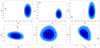 |
Fig. 5. Same as Fig. 4, but for a reference flat ΛCDM model with ΩM, 0 = 0.7. |
| In the text | |
|
Fig. 6. Deviations (in unity of σ) of the cosmographic distance moduli of quasars (yellow bars) and SNe (blue bars) from the best-fit ΛCDM model up to z = 1.1 and extrapolated to higher redshifts. The values of σ are redshift-averaged in narrow logarithmic bins. A discrepancy between the data and the model emerges at z ≥ 1 and it remains significant at higher redshifts. This proves the tension between the ΛCDM model and the observations. |
| In the text | |
|
Fig. 7. Top panel: hubble diagram of SNe (cyan points) and quasars (yellow points). The red points are averages (along with their uncertainties) of the distance moduli of quasars in narrow (logarithmic) redshift intervals and they are shown for visualization purposes only, without any statistical application. Dashed magenta and continuous black lines show respectively the best-fit curves of the flat ΛCDM and the logarithmic models over the whole redshift range. Bottom panel: residuals with respect to the cosmographic fit for quasars and averages of the residuals over the same redshift intervals. |
| In the text | |
Current usage metrics show cumulative count of Article Views (full-text article views including HTML views, PDF and ePub downloads, according to the available data) and Abstracts Views on Vision4Press platform.
Data correspond to usage on the plateform after 2015. The current usage metrics is available 48-96 hours after online publication and is updated daily on week days.
Initial download of the metrics may take a while.