| Issue |
A&A
Volume 649, May 2021
|
|
|---|---|---|
| Article Number | A91 | |
| Number of page(s) | 9 | |
| Section | Stellar structure and evolution | |
| DOI | https://doi.org/10.1051/0004-6361/202040149 | |
| Published online | 18 May 2021 | |
KMT-2019-BLG-0797: Binary-lensing event occurring on a binary stellar system
1
Department of Physics, Chungbuk National University, Cheongju 28644, Republic of Korea
e-mail: This email address is being protected from spambots. You need JavaScript enabled to view it.
2
Korea Astronomy and Space Science Institute, Daejon 34055, Republic of Korea
3
University of Canterbury, Department of Physics and Astronomy, Private Bag 4800, Christchurch 8020, New Zealand
4
Korea University of Science and Technology, 217 Gajeong-ro, Yuseong-gu, Daejeon 34113, Republic of Korea
5
Max Planck Institute for Astronomy, Königstuhl 17, 69117 Heidelberg, Germany
6
Department of Astronomy, The Ohio State University, 140 W. 18th Ave., Columbus, OH 43210, USA
7
Department of Particle Physics and Astrophysics, Weizmann Institute of Science, Rehovot 76100, Israel
8
Center for Astrophysics | Harvard & Smithsonian, 60 Garden St., Cambridge, MA 02138, USA
9
Department of Astronomy, Tsinghua University, Beijing 100084, PR China
10
School of Space Research, Kyung Hee University, Yongin, Kyeonggi 17104, Republic of Korea
Received:
16
December
2020
Accepted:
2
February
2021
Abstract
Aims. We analyze the microlensing event KMT-2019-BLG-0797. The light curve of the event exhibits two anomalous features from a single-lens single-source model, and we aim to reveal the nature of the anomaly.
Methods. It is found that a model with two lenses plus a single source (2L1S model) can explain one feature of the anomaly, but the other feature cannot be explained. We test various models and find that both anomalous features can be explained by introducing an extra source to a 2L1S model (2L2S model), making the event the third confirmed case of a 2L2S event, following MOA-2010-BLG-117 and OGLE-2016-BLG-1003. It is estimated that the extra source comprises ∼4% of the I-band flux from the primary source.
Results. Interpreting the event is subject to a close–wide degeneracy. According to the close solution, the lens is a binary consisting of two brown dwarfs with masses (M1, M2) ∼ (0.034, 0.021) M⊙, and it is located at a distance of DL ∼ 8.2 kpc. According to the wide solution, on the other hand, the lens is composed of an object at the star–brown dwarf boundary and an M dwarf with masses (M1, M2) ∼ (0.06, 0.33) M⊙ located at DL ∼ 7.7 kpc. The source is composed of a late G dwarf to early K dwarf primary and an early-to-mid M dwarf companion.
Key words: gravitational lensing: micro
© ESO 2021
1. Introduction
Microlensing light curves can exhibit deviations from the smooth and symmetric form of a single-lens single-source (1L1S) event. The most common causes for these anomalies are the binary natures of the lens, 2L1S event (Mao & Paczyński 1991), and the source, 1L2S event (Griest & Hu 1992). Detections of such three-object (2L plus 1S or 1L plus 2S) events by the first-generation lensing experiments, for example, the MACHO LMC 1 (Dominik & Hirshfeld 1994) and OGLE 7 (Udalski et al. 1994) 2L1S events and the MACHO LMC 96-2 (Becker et al. 1997) 1L2S event, prompted theoretical studies on the lensing behavior under these lens system configurations. This led to the establishment of observational strategies for efficient detections of microlensing anomalies, such as survey plus follow-up mode observations for intensive coverage of short-lasting anomalies (Gould & Loeb 1992), and the development of methodologies for efficient analyses of anomalous lensing events, such as the ray-shooting method (Bond et al. 2002; Dong et al. 2009; Bennett et al. 2010) and the contour integration algorithm (Gould & Gaucherel 1997; Bozza et al. 2018). Thanks to accomplishments on both observational and theoretical sides, more than a hundred anomalous events are currently being detected each year, and they are promptly analyzed in almost real time with the progress of events (Ryu et al. 2010; Bozza et al. 2012).
With the great increase in the event detection rate together with the dense coverage of lensing light curves by the high-cadence lensing surveys, for example, the fourth phase of the Optical Gravitational Lensing Experiment (OGLE-IV: Udalski et al. 2015), the Microlensing Observations in Astrophysics survey (MOA: Bond et al. 2001), and the Korea Microlensing Telescope Network survey (KMTNet: Kim et al. 2016), one is occasionally confronted with events for which observed lensing light curves cannot be explained via interpretations with three objects. At the time of writing this article, there exist 13 confirmed cases of events for which at least four objects (lenses plus sources) are required to interpret observed light curves. These events are listed in Table 1. Nine of these are 3L1S events, in which the lensing system is composed of three lens masses and a single source star. Among them, the lenses of six events (OGLE-2008-BLG-092, OGLE-2007-BLG-349, OGLE-2013-BLG-0341, OGLE-2016-BLG-0613, OGLE-2018-BLG-1700, and OGLE-2019-BLG-0304) are planets in binaries, and the lenses of the other three events (OGLE-2006-BLG-109, OGLE-2012-BLG-0026, and OGLE-2018-BLG-1011) are systems containing two planets. The lensing event OGLE-2015-BLG-1459 was identified as a 1L3S event, in which a single-lens mass was involved with three source stars. The events MOA-2010-BLG-117 and OGLE-2016-BLG-1003 were very rare cases, in which both the lens and source are binaries. Interpretation of the event KMT-2019-BLG-1715 is even more complex and requires five objects, in which the lens is composed of three masses (a planet plus two stars) and the source consists of two stars, that is, a 3L2S event. Besides these events, there exist three additional events (OGLE-2014-BLG-1722, OGLE-2018-BLG-0532, and KMT-2019-BLG-1953) for which four-object modeling is required to explain the observed light curves, but unique solutions cannot be firmly specified due to either degeneracies among different interpretations or an insufficient coverage of signals. Accumulation of knowledge from modeling these multi-body events is important for future interpretations of lensing light curves with complex anomalous features.
Microlensing events with more than four bodies.
In this paper, we present the analysis of the lensing event KMT-2019-BLG-0797. The light curve of the event exhibits two anomalous features that cannot be explained by a usual 2L1S or 1L2S model. We test various four-object models, in which an extra lens or source are considered in the interpretation of the event.
The anomalous nature of KMT-2019-BLG-0797 was found from a project conducted to reanalyze previous KMTNet events detected in and before the 2019 season. In the first part of this project, Han et al. (2020c) investigated events involving with faint source stars and found four planetary events (KMT-2016-BLG-2364, KMT-2016-BLG-2397, OGLE-2017-BLG-0604, and OGLE-2017-BLG-1375) for which no detailed investigation had been conducted. The second part of the project was focused on high-magnification events, aiming to find subtle planetary signals, and this led to the discoveries of two planetary systems, KMT-2018-BLG-0748L (Han et al. 2020d) and KMT-2018-BLG-1025L (Han et al. 2021c). The event KMT-2019-BLG-0797 was closely examined as a part of the project investigating high-magnification events involving with faint source stars.
For the presentation of this work, we organize the paper as follows. In Sect. 2, we present the data of the lensing event analyzed in this work and describe the observations conducted to acquire the data. In Sect. 3, we depict the anomaly that appeared on the light curve and describe various tests conducted to interpret the anomaly. We estimate the angular Einstein radius of the lensing event in Sect. 4 and estimate the physical parameters of the lens and source in Sect. 5. We summarize the results and conclude in Sect. 6.
2. Observation and data
The lensing event KMT-2019-BLG-0797 occurred on a source lying toward the Galactic bulge. The equatorial and galactic coordinates of the source are (RA, Dec)J2000 = (17 : 53 : 48.09, −31 : 58 : 36.70) and  , respectively. The brightness of the source had remained constant with an apparent baseline brightness of Ibase ∼ 20.1, as measured on the KMTNet scale, before the lensing magnification. The lensing-induced magnification of the source flux lasted about 10 days as measured by the duration beyond the photometric scatter.
The event was detected on 2019 May 13 (HJD′≡HJD − 2 450 000 ∼ 8616.6) by the Alert Finder System (Kim et al. 2018) of the KMTNet survey. The survey uses three identical wide-field telescopes that are globally located on three continents. The locations of the individual telescopes are the Siding Spring Observatory (KMTA) in Australia, the Cerro Tololo Inter-American Observatory (KMTC) in South America, and the South African Astronomical Observatory (KMTS) in Africa. Each KMTNet telescope has a 1.6 m aperture and is equipped with a camera yielding a 2° ×2° field of view. Images of the source were mainly acquired in the I-band, and about one tenth of images were obtained in the V-band for the source color measurement. We will describe the detailed procedure of determining the source color in Sect. 4.
Figure 1 shows the lensing light curve of KMT-2019-BLG-0797. The curve plotted over the data points is a 1L1S model with (t0, u0, tE) ∼ (8617.06, 0.20, 4.6 days), where the individual lensing parameters indicate the peak time, impact parameter of the lens-source approach (normalized to the angular Einstein radius θE), and event timescale, respectively. The inset shows a zoomed-in view of the peak region, around which the data exhibit an anomaly relative to the 1L1S model. The date of the event alert approximately corresponds to the peak of the lensing magnification. The anomaly was already in progress at the time of the event alert, but it was not noticed due to the subtlety of the anomaly together with the considerable photometric uncertainties of data caused by the faintness of the source. As a result, little attention was paid to the event when it was found, and thus no alert for follow-up observations was issued. Nevertheless, the peak region of the light curve was densely and continuously covered because the source was located in the two overlapping KMTNet fields of BLG01 and BLG41, toward which observations were conducted most frequently. The observational cadence for each field was 30 min, and thus the event was covered with a combined cadence of 15 min.
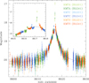 |
Fig. 1. Light curve of KMT-2019-BLG-0797. The curve drawn over the data points is a 1L1S model. The inset shows the region around the peak. The colors of the data points match those of the telescopes, marked in the legend, used to acquire the data. |
Photometry of the event was conducted utilizing the KMTNet pipeline (Albrow et al. 2009), which is a customized version of pySIS code developed on the basis of the difference imaging method (Tomaney & Crotts 1996; Alard & Lupton 1998). Additional photometry was conducted for a subset of KMTC I- and V-band data using the pyDIA software (Albrow 2017) to measure the color of the source and to construct a color-magnitude diagram (CMD) of ambient stars around the source. We readjusted error bars of data estimated from the pipeline following the standard routine described in Yee et al. (2012).
3. Anomaly
Figure 2 shows the detailed pattern of the anomaly in the peak region. It shows that the anomaly consists of two distinctive features. The first is the caustic-crossing feature, which is composed of two spikes at HJD′∼8616.3 and 8616.7 and a U-shape trough between the spikes. The other feature is the strong positive deviation from the 1L1S model centered at HJD′∼8617.2. The KMTA data partially cover the rising side of the second feature, but the falling side was not covered until almost the end of the anomaly.
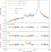 |
Fig. 2. Zoomed-in view around the peak of the light curve. Drawn over the data points are the 2L2S (wide), 3L1S, and 2L1S models. The lower three panels show the residuals from the individual models. |
3.1. 2L1S model
Considering that both anomalous features are likely to be involved with the source star’s crossing over or approaching a caustic, we first modeled the observed light curve under the assumption that the lens is a binary. In addition to the 1L1S lensing parameters, a 2L1S modeling requires the inclusion of the three additional parameters (s, q, α), which represent the projected separation (normalized to θE), the mass ratio between the binary lens components (M1 and M2), and the angle between the source trajectory and the M1 − M2 axis (source trajectory angle), respectively. In the 2L1S modeling, we conducted thorough grid searches for the binary parameters (s, q) with multiple starting points of α evenly distributed in the range of 0 ≤ α ≤ 2π. For the computations of finite-source magnifications, we used the ray-shooting method described in Dong et al. (2009). From our investigation, we find that the 2L1S modeling does not yield a plausible model explaining the observed anomalous features.
We then conducted another 2L1S modeling, this time by excluding the data around one of the two anomaly features. The modeling conducted by removing the data around the second anomalous feature does not yield a reasonable solution either1. However, the modeling with the exclusion of the first anomalous feature yields a solution that describes the second anomalous feature well.
The model curve of the 2L1S solution obtained by excluding the first anomalous feature is plotted over the data points in Fig. 2, and the lensing parameters of the solution are listed in Table 2. We find two sets of solutions: One has a binary separation smaller than unity (s < 1.0), and the other has a separation greater than unity (s > 1.0). We refer to the two solutions as the “close” and “wide” solutions, respectively. The binary parameters of the close and wide solutions are (s, q, α)close ∼ (0.52, 0.60, −6.6° ) and (s, q, α)wide ∼ (3.62, 5.75, −100.8° ), respectively. We note that M1 denotes the lens component located closer to the source trajectory, not the heavier mass component, and thus the mass ratio q of the wide solution is greater than unity. For the wide solution, we present additional parameters  , which represent the values scaled to the angular Einstein radius corresponding to M1,
  , and thus
  ,
,  , and ρ′=ρ(1 + q)1/2. We find that parameters
  of the wide solution are similar to the corresponding parameters of the close solution.
Best-fit parameters of 2L1S solutions.
Figure 3 shows the configuration of the lens system corresponding to the 2L1S solutions. The upper and lower panels are the configurations of the close and wide solutions, respectively. According to these solutions, the second feature of the anomaly is produced by the source crossing over the tip of the four-cusp caustic that was induced by a binary. We note that the binary separations of the lens, s ∼ 0.52 for the close solution and s ∼ 2.6 for the wide solution, are neither much smaller nor much greater than unity; thus, the lens system is not in the regime of Chang–Refsdal (C–R) lensing, which refers to the gravitational lensing of a point mass perturbed by a constant external shear (Chang & Refsdal 1979, 1984). As a result, the caustic slightly deviates from the symmetric astroid shape of the C–R lensing caustic. The source crosses the caustic tip located on the long side of the caustic.
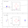 |
Fig. 3. Lens system configurations of the 2L1S solutions. The upper and lower panels are for the close and wide solutions, respectively. The inset in each panel shows the enlarged view around the caustic located close to the source trajectory (line with an arrow). The blue dots marked M1 and M2 denote the positions of the binary lens components, and the bigger dot represents the heavier lens mass. Lengths are scaled to the Einstein radius. The small magenta circle on the source trajectory represents the source size scaled to the Einstein radius: ρ = θ*/θE. |
3.2. 2L2S model
We conducted another modeling under the interpretation that both the lens and source are binaries (2L2S model). The lensing magnification of a 2L2S event is the superposition of those involved with the individual source stars, S1 and S2, that is,
 (1)
(1)
Here (FS1, FS2) and (A1, A2) denote the baseline flux values and the magnifications associated with the individual source stars, respectively, and qF = FS2/FS1 represents the flux ratio between the source stars. The consideration of an extra source requires the inclusion of additional parameters in modeling. These parameters are (t0, 2, u0, 2, ρ2, qF), which represent the time of the closest approach of S2 to the lens, the lens-source separation at that time, the normalized radius of S2, and the flux ratio between S1 and S2, respectively (Hwang et al. 2013). As initial values of the parameters related to S1, (t0, 1, u0, 1, tE, s, q, α, ρ1), we used the values obtained from the 2L1S modeling. We set the initial values of (t0, 2, u0, 2, ρ2, qF) considering the time and strength of the first anomaly feature.
We find that the 2L2S modeling yields solutions that describe the observed data well, including both anomalous features. We find two sets of solutions resulting from the close–wide degeneracy, and the best-fit lensing parameters of the individual solutions are listed in Table 3. The wide solution yields a slightly better fit to the data than the close solution, especially in the region around the second anomalous feature. However, the χ2 difference between the two solutions is merely Δχ2 = 5.5, and thus we consider the close solution as a viable model. The model curves of the wide solution and the residual from the model are shown in Fig. 2.
Best-fit parameters of 2L2S solutions.
In Fig. 4, we present the lens system configurations corresponding to the close (upper panel) and wide (lower panel) 2L2S solutions. From the comparison of the lensing parameters with those of the 2L1S solutions, presented in Table 2, it is found that the parameters related to S1 for the 2L1S and 2L2S solutions, (t0, 1, u0, 1, tE, s, q, α), are similar to each other. The main difference between the two solutions is the presence of an additional source, S2, which approaches M1 more closely than S1 does. The second source passes over the caustic, producing a caustic-crossing feature in the light curve, and this explains the first anomalous feature that could not be explained by the 2L1S model. According to the 2L2S solutions, the companion source comprises about 4% of the I-band flux from the primary source, that is, qF, I ∼ 0.04.
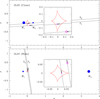 |
Fig. 4. Lens system configuration of the 2L2S model. Notations are same as those in Fig. 3 except that there is an additional source trajectory of the second source, S2. |
We note that the source trajectory of the event is well constrained despite the approximately symmetric shape of the caustic. For a binary lens in a C–R lensing regime, the induced caustic has a symmetric astroid shape with four cusps. In this case, the lensing light curves resulting from the source trajectory angles α and α ± 90° have a similar shape. An illustration of this degeneracy is shown in Fig. 4 of Hwang et al. (2010). We find that KMT-2019-BLG-0797 is not subject to this degeneracy because the source trajectory of the solution with α ± 90° is approximately aligned with the line connecting the central and peripheral caustics of the binary lens. To demonstrate this, in Fig. 5, we plot the lens system configurations of the solutions obtained by confining the source trajectory angle around ∼α ± 90° from the best-fit solution. It shows that these solutions result in source trajectories passing close to the peripheral caustic that lies away from the central caustic. The source approach to the peripheral caustic results in an additional bump in the lensing light curve before the main peak. To avoid such a bump, the source trajectory angle of these solutions has less freedom in α, and this leads to a worse fit than the solutions presented in Table 3.
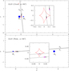 |
Fig. 5. Lens system configuration of the models obtained by confining the source trajectory angle around ∼α + 90° from the best-fit solutions with α. |
3.3. 3L1S model
We also tested a model in which the lens has three components (3L1S model). We tested this model because the anomalous features appear around the peak of the light curve, and thus a third mass, if it exists, may induce an additional caustic and explain the first anomalous feature that is not explained by a 2L1S model, for example OGLE-2016-BLG-0613 (Han et al. 2017), OGLE-2018-BLG-1700 (Han et al. 2020a), and OGLE-2019-BLG-0304 (Han et al. 2021b). In the 3L1S modeling, we conducted a thorough grid search for the parameters that describe the third lens mass, M3. These parameters include (s3, q3, ψ), which denote the normalized M1 − M3 separation, the mass ratio q3 = M3/M1, and the position angle of M3 as measured from the M1 − M2 axis and with a center at M1.
The 3L1S modeling also yields a solution that appears to depict both anomalous features. In Fig. 2, we present the model curve and residual in the peak region of the light curve. The best-fit lensing parameters of the model are listed in Table 4, and the corresponding lens system configuration is shown in Fig. 6. According to this solution, the first anomalous feature is produced by the crossing of the source over an additional caustic that is induced by a low-mass third-lens component. The estimated mass ratio of the third mass to the primary is q3 = M3/M1 = (2.75 ± 0.28) × 10−3, indicating that M3 is a planetary mass object. The planet is located close to the Einstein ring that corresponds to M1 + M2 with a position angle of ψ ∼ 64°. Due to the proximity of s3 to unity, the planet induces a single large resonant caustic and the source passes through the planet-induced caustic. This produces the first anomalous feature before it approaches the cusp of the binary-induced caustic, producing, in turn, the second anomalous feature.
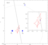 |
Fig. 6. Lens system configuration of the 3L1S model. We note that there are three lens components, marked M1, M2, and M3. The dotted circle with a radius unity and centered at the M1 − M2 barycenter represents the Einstein ring. |
Best-fit parameters of 3L1S solution.
Although the 3L1S model seemingly describes the anomalous features, it is found that the model fit is substantially worse than that of the 2L2S model. The difference in the fits between the two models as measured by the χ2 difference is  , indicating that the 2L2S model is strongly preferred over the 3L1S model. To show the difference in the fits, we present the cumulative distribution of Δχ2 between the two models in Fig. 7. The distribution shows that the 2L2S model provides a better fit than the 3L1S model not only in the region around the peak but also throughout the light curve during the lensing magnification.
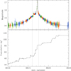 |
Fig. 7. Cumulative distribution of the χ2 difference between the 3L1S and 2L2S models, that is, |
4. Angular Einstein radius
In this section, we estimate the angular Einstein radius θE. In order to estimate θE, it is required to measure the normalized source radius, which is related to the angular Einstein radius by
 (2)
(2)
Here θ* represents the angular source radius. We find that the normalized source radii of both S1 and S2 are constrained, although the uncertainties are considerable due to a partial coverage of the caustic crossings. This can be seen in Fig. 8, in which we present scatter plots of the points in the Markov chain Monte Carlo (MCMC) chain on the ρ1 − ρ2 parameter plane for the close (left panel) and wide (right panel) solutions. We note that the uncertainty of ρ1 is greater than the uncertainty of ρ2 due to the fact that only the rising part of the second anomalous feature was covered by the data.
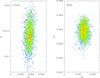 |
Fig. 8. Scatter plots in the MCMC chain on the ρ1 − ρ2 parameter plane for the close (left panel) and wide (right panel) solutions. The color coding is set to indicate points within 1σ (red), 2σ (yellow), 3σ (green), 4σ (cyan), and 5σ (blue). |
Another requirement for the θE measurement is an estimation of the angular source radius θ*. We estimated θ* from the color and brightness of the source. In order to estimate calibrated color and brightness from the instrumental values, we used the method in Yoo et al. (2004). In this method, the centroid of the red giant clump (RGC), with its known de-reddened color and magnitude, in the CMD serves as a reference for the color and magnitude calibration.
In the first step of the method, we estimated the combined (instrumental) flux from the source stars, FS, p = FS1, p + FS2, p, and the companion/primary flux ratio, qF, p, by fitting the KMTC photometry data set processed using the pyDIA code. Here the subscript “p” denotes the passband of observation. The measured values are (FS, I, FS, V) = (0.07751 ± 0.00060, 0.00909 ± 0.00032) and (qF, I, qF, V) = (0.0471 ± 0.0023, 0.0110 ± 0.0084). We note that the value of qF, I, which is derived from the pyDIA reduction, is slightly different (less than 1σ) from the value presented in Table 3, which is derived from the pySIS reduction, because they come from different reductions of the data. Then, the flux values from S1 and S2 were estimated by
 (3)
(3)
respectively. From the measured flux values in the I- and V-bands, we estimated the colors and magnitudes of S1 and S2 to be (V − I, I)S1 = (2.289 ± 0.043, 20.827 ± 0.010) and (V − I, I)S2 = (3.868 ± 0.831, 24.143 ± 0.053), respectively. In Fig. 9, we mark the locations of S1 and S2 with respect to the RGC centroid in the instrumental CMD that was constructed using the pyDIA photometry of the KMTC data (gray dots).
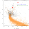 |
Fig. 9. Locations of the primary and companion source stars with respect to the centroid of the RGC in the instrumental CMD (gray dots). The determinations of the source positions and the construction of the CMD are based on the pyDIA photometry of the KMTC data set. We also present the Hubble Space Telescope CMD (Holtzman et al. 1998, brown dots) to show the source locations on the main-sequence branch. |
Although the V-band flux of S2 has a relatively large fractional (magnitude) error, it is strongly constrained to be faint in an absolute sense. In particular, we find
 (4)
(4)
(i.e., a 4.4σ difference). This serves as a second line of evidence that the 2L2S solution is correct. If, for example, we had somehow missed a 3L1S solution, and the derived 2L2S solutions were merely mimicking it, then qF, I − qF, V should be consistent with zero because there is only one source with just one color. However, according to Eq. (4), this possibility is excluded at 4.4σ.
In the second step, we calibrated the color and magnitude. With the measured instrumental color and brightness of the source, (V − I, I), and the RGC centroid, (V − I, I)RGC = (2.473, 16.918), together with the known de-reddened values of the RGC centroid, (V − I, I)RGC, 0 = (1.060, 14.509) (Bensby et al. 2013; Nataf et al. 2013), the reddening and extinction corrected color and magnitude of the source were estimated by
 (5)
(5)
where Δ(V − I, I) denote the offsets in the color and brightness of the source from the RGC centroid measured on the instrumental CMD. This results in
 (6)
(6)
In Table 5, we summarize the values of (V − I, I)RGC, (V − I, I)RGC, 0, (V − I, I), and (V − I, I)0 for the primary and companion source stars.
Source color and magnitude.
According to the estimated color and magnitude, the fainter source, S2, is clearly an early-to-mid M dwarf. On the other hand, the brighter source, S1, presents something of a puzzle because its best-fit position lies in a relatively unpopulated portion of the CMD (see Fig. 9). The most likely explanation is that its true position lies (1.5−2.0)σ blueward of the best-fit position. That is, it is most likely a very late G dwarf or a very early K dwarf. Because the position of S1 is consistent with lying in the normal bulge population at the (1−2)σ level, we evaluated its angular radius using the measured values and normal error propagation.
In the third step, we estimated the angular source radius using the measured source color and brightness. For this, we first converted V − I color into V − K color using the color–color relation from Bessell & Brett (1988) and then estimated θ* using the (V − K)−θ* relation from Kervella et al. (2004). This process yields an angular source radius of
 (7)
(7)
We note that the source radius of S2 is uncertain due to its large color uncertainty, and thus we used θ* of S1 for the θE estimation (i.e., θE = θ*, 1/ρ1). With the angular source radius, the angular Einstein radius was estimated using the relation in Eq. (2), which yields
 (8)
(8)
Here the angular Einstein radius of the wide solution is scaled to  . Together with the event timescale, the relative lens-source proper motion was estimated as
 (9)
(9)
In Table 6, we summarize the values of θ*, θE, and μ that correspond to the close and wide solutions.
Angular source radius, Einstein radius, and proper motion.
5. Physical parameters of the lens and source
For KMT-2019-BLG-0797, it is difficult to uniquely determine the physical lens parameters because the microlens parallax cannot be measured due to the short timescale of the event, which is ≲5 days. However, the lens parameters can still be constrained with the measured observables of the event timescale and angular Einstein radius because these observables are related to the lens parameters by
 (10)
(10)
Here κ = 4G/(c2AU), πrel denotes the relative lens-source parallax and DL and DS represent the distances to the lens and the source, respectively.
We estimated the physical lens parameters by conducting a Bayesian analysis. The analysis was done using the priors of the lens mass function and the physical and dynamical galactic models. We adopted the mass function models from Zhang et al. (2020) and Gould (2000); the former includes stellar and brown-dwarf lenses, and the latter accounts for stellar remnants. The locations and motions of lenses and source stars were assigned using the physical distribution model from Han & Gould (2003) and the dynamical distribution model from Han & Gould (1995), respectively. Based on these models, we produced a large number (4 × 10⁷) of artificial lensing events by conducting a Monte Carlo simulation and then constructed the distributions of the physical parameters. With the distributions, the representative values of the lens parameters were estimated as the median values of the distributions, and the uncertainties were estimated as the 16% and 84% ranges of the distributions.
Figure 10 shows the Bayesian posteriors of the primary lens mass and the distances to the lens and source. In Table 7, we list the estimated parameters M1, M2, DL, DS, aL, ⊥, and aS, ⊥. The last two parameters indicate the projected binary-lens and binary-source separations, that is,
 (11)
(11)
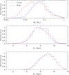 |
Fig. 10. Bayesian posteriors of the primary lens mass (M1) as well as distances to the lens (DL) and source (DS). Red and blue curves are distributions obtained from the close and wide solutions, respectively. |
Physical lens parameters.
where Δu = {[(t0, 1 − t0, 2)/tE]2 + (u0, 1 − u0, 2)2}1/2 is the instantaneous separation between S1 and S2 at the time of the lensing magnification.
According to the close solution, the lens is composed of two brown dwarfs with masses (M1, M2) ∼ (0.034, 0.021) M⊙ located in the bulge with a distance of  kpc. According to the wide solution, on the other hand, the lens is composed of an object at the star–brown dwarf boundary and an M dwarf with masses (M1, M2) ∼ (0.06, 0.33) M⊙, and it is located at a distance of
  kpc. The masses of M1 estimated from the close and wide solutions are similar to each other, although the wide solution prefers a somewhat larger mass due to the larger value of the estimated θE. On the other hand, the masses of M2 estimated from the two degenerate solutions differ widely. This is because M1 and M2 have similar masses, with q ∼ 0.6, according to the close solution, while M2, according to the wide solution, is much heavier than M1, with q ∼ 5.3. For both the close and wide solutions, the source is located slightly behind the galactic center at a distance of DS ∼ 9.1 kpc. This is because source stars located on the far side of the bulge have higher chances of being lensed than stars located on the front side. The projected separations between the lens and source components are (aL, ⊥, aS, ⊥) ∼ (0.26, 0.10) AU, according to the close solution, and ∼(2.68, 0.06) AU, according to the wide solution. We note that the expected orbital periods of the source, P ≳ 10.5 days for the close solution and P ≳ 5 days for the wide solution with the source mass of MS = MS1 + MS2 ∼ 0.9 M⊙ + 0.3 M⊙ ∼ 1.2 M⊙, is short, and thus the orbital motion of the source may affect the lensing light curve. However, it is difficult to constrain the orbital motion because, firstly, the duration of the anomaly, which is ∼1 day, is much shorter than the orbital period and, secondly, because the photometric precision in the wings of the light curve is not good enough to capture the small modulations induced by the source orbital motion.
6. Summary and conclusion
We investigated the lensing event KMT-2019-BLG-0797, for which the light curve was found to be anomalous from a reexamination of events detected in and before the 2019 season. For this event, we found that a 2L1S model could not explain the anomaly. From the tests with various models, we found that the anomaly could be explained by introducing an extra source star to a 2L1S model. This event is the third case of a confirmed 2L2S event, following MOA-2010-BLG-117 (Bennett et al. 2018) and OGLE-2016-BLG-1003 (Jung et al. 2017).
The interpretation of the light curve was subject to a close–wide degeneracy. According to the close solution, the lens is a binary consisting of two brown dwarfs with masses (M1, M2) ∼ (0.034, 0.021) M⊙, and it is located at a distance of DL ∼ 8.2 kpc. According to the wide solution, on the other hand, the lens is composed of an object at the star–brown dwarf boundary and an M dwarf with masses (M1, M2) ∼ (0.06, 0.33) M⊙ located at DL ∼ 7.7 kpc. The binary source comprises a primary near the G dwarf–K dwarf boundary and an early-to-mid M dwarf companion.
As we will show in the following subsection, the first anomalous feature is produced by an extra source. This source comprises a very minor fraction of the primary source, and the most flux comes from the primary source. As a result, the contribution of the second source to the lensing light curve is confined only to the time of the first anomaly, and thus the 2L1S modeling conducted excluding the second anomalous feature does not yield a model describing the overall light curve.
Acknowledgments
Work by C.H. was supported by the grants of National Research Foundation of Korea (2019R1A2C2085965 and 2020R1A4A2002885). This research has made use of the KMTNet system operated by the Korea Astronomy and Space Science Institute (KASI) and the data were obtained at three host sites of CTIO in Chile, SAAO in South Africa, and SSO in Australia.
References
- Alard, C., & Lupton, R. H. 1998, ApJ, 503, 325 [NASA ADS] [CrossRef] [Google Scholar]
- Albrow, M. 2017, https://doi.org/10.5281/zenodo.268049 [Google Scholar]
- Albrow, M., Horne, K., Bramich, D. M., et al. 2009, MNRAS, 397, 2099 [NASA ADS] [CrossRef] [Google Scholar]
- Becker, A., Alcock, C., Allsman, R., et al. 1997, BAAS, 29, 1347 [Google Scholar]
- Bennett, D. P., Rhie, S. H., Nikolaev, S., et al. 2010, ApJ, 713, 837 [NASA ADS] [CrossRef] [Google Scholar]
- Bennett, D. P., Rhie, S. H., Udalski, A., et al. 2016, AJ, 152, 125 [NASA ADS] [CrossRef] [Google Scholar]
- Bennett, D. P., Udalski, A., Han, C., et al. 2018, AJ, 155, 141 [Google Scholar]
- Bensby, T., Yee, J. C., Feltzing, S., et al. 2013, A&A, 549, A147 [NASA ADS] [CrossRef] [EDP Sciences] [Google Scholar]
- Bessell, M. S., & Brett, J. M. 1988, PASP, 100, 1134 [NASA ADS] [CrossRef] [Google Scholar]
- Bozza, V., Dominik, M., Rattenbury, N. J., et al. 2012, MNRAS, 424, 902 [NASA ADS] [CrossRef] [Google Scholar]
- Bozza, V., Bachelet, E., Bartolić, F., et al. 2018, MNRAS, 479, 5157 [Google Scholar]
- Bond, I. A., Abe, F., Dodd, R. J., et al. 2001, MNRAS, 327, 868 [Google Scholar]
- Bond, I. A., Rattenbury, N. J., Skuljan, J., et al. 2002, MNRAS, 333, 71 [NASA ADS] [CrossRef] [Google Scholar]
- Chang, K., & Refsdal, S. 1979, Nature, 282, 561 [Google Scholar]
- Chang, K., & Refsdal, S. 1984, A&A, 132, 168 [NASA ADS] [Google Scholar]
- Dominik, M., & Hirshfeld, A. C. 1994, A&A, 289, L31 [Google Scholar]
- Dong, S., Bond, I. A., Gould, A., et al. 2009, ApJ, 698, 1826 [NASA ADS] [CrossRef] [Google Scholar]
- Gaudi, B. S., Bennett, D. P., Udalski, A., et al. 2008, Science, 319, 927 [NASA ADS] [CrossRef] [PubMed] [Google Scholar]
- Gould, A. 2000, ApJ, 535, 928 [NASA ADS] [CrossRef] [Google Scholar]
- Gould, A., & Gaucherel, C. 1997, ApJ, 477, 580 [Google Scholar]
- Gould, A., & Loeb, A. 1992, ApJ, 396, 104 [NASA ADS] [CrossRef] [Google Scholar]
- Gould, A., Udalski, A., Shin, I.-G., et al. 2014, Science, 345, 46 [NASA ADS] [CrossRef] [Google Scholar]
- Griest, K., & Hu, W. 1992, ApJ, 397, 362 [NASA ADS] [CrossRef] [Google Scholar]
- Han, C., & Gould, A. 1995, ApJ, 447, 53 [NASA ADS] [CrossRef] [Google Scholar]
- Han, C., & Gould, A. 2003, ApJ, 592, 172 [NASA ADS] [CrossRef] [Google Scholar]
- Han, C., Udalski, A., Choi, J.-Y., et al. 2013, ApJ, 762, L28 [NASA ADS] [CrossRef] [Google Scholar]
- Han, C., Udalski, A., Gould, A., et al. 2017, AJ, 154, 223 [Google Scholar]
- Han, C., Bennett, D. P., Udalski, A., et al. 2019, AJ, 158, 114 [Google Scholar]
- Han, C., Lee, C.-U., Udalski, A., et al. 2020a, AJ, 159, 48 [Google Scholar]
- Han, C., Kim, D., Jung, Y. K., et al. 2020b, AJ, 160, 17 [Google Scholar]
- Han, C., Udalski, A., Kim, D., et al. 2020c, A&A, 642, A110 [EDP Sciences] [Google Scholar]
- Han, C., Shin, I.-G., Jung, Y. K., et al. 2020d, A&A, 641, A105 [CrossRef] [EDP Sciences] [Google Scholar]
- Han, C., Udalski, A., Kim, D., et al. 2021a, AJ, submitted [arXiv:2104.00293] [Google Scholar]
- Han, C., Udalski, A., Lee, C.-U., et al. 2021b, AJ, submitted [Google Scholar]
- Han, C., Udalski, A., Lee, C.-U., et al. 2021c, A&A, 649, A90 [EDP Sciences] [Google Scholar]
- Holtzman, J. A., Watson, A. M., Baum, W. A., et al. 1998, AJ, 115, 1946 [NASA ADS] [CrossRef] [Google Scholar]
- Hwang, K.-H., Han, C., Bond, I. A., et al. 2010, ApJ, 717, 435 [Google Scholar]
- Hwang, K.-H., Choi, J.-Y., Bond, I. A., et al. 2013, ApJ, 778, 55 [NASA ADS] [CrossRef] [Google Scholar]
- Hwang, K.-H., Udalski, A., Bond, I. A., et al. 2018, AJ, 155, 259 [Google Scholar]
- Jung, Y. K., Udalski, A., Bond, I. A., et al. 2017, ApJ, 841, 75 [Google Scholar]
- Kervella, P., Thévenin, F., Di Folco, E., & Ségransan, D. 2004, A&A, 426, 29 [Google Scholar]
- Kim, S.-L., Lee, C.-U., Park, B.-G., et al. 2016, J. Korean Astron. Soc., 49, 37 [Google Scholar]
- Kim, H.-W., Hwang, K.-H., Shvartzvald, Y., et al. 2018, AJ, 155, 76 [NASA ADS] [CrossRef] [Google Scholar]
- Mao, S., & Paczyński, B. 1991, ApJ, 374, L37 [Google Scholar]
- Nataf, D. M., Gould, A., Fouqué, P., et al. 2013, ApJ, 769, 88 [NASA ADS] [CrossRef] [Google Scholar]
- Poleski, R., Skowron, J., Udalski, A., et al. 2014, ApJ, 795, 42 [Google Scholar]
- Ryu, Y.-H., Han, C., Hwang, K.-H., et al. 2010, ApJ, 723, 81 [NASA ADS] [CrossRef] [Google Scholar]
- Ryu, Y.-H., Udalski, A., Yee, J. C., et al. 2020, AJ, 160, 183 [Google Scholar]
- Suzuki, D., Bennett, D. P., Udalski, A., et al. 2018, AJ, 155, 263 [Google Scholar]
- Tomaney, A. B., & Crotts, A. P. S. 1996, AJ, 112, 2872 [NASA ADS] [CrossRef] [Google Scholar]
- Udalski, A., Szymański, M., Mao, S., et al. 1994, ApJ, 436, L103 [NASA ADS] [CrossRef] [Google Scholar]
- Udalski, A., Szymański, M. K., & Szymański, G. 2015, Acta Astron., 65, 1 [NASA ADS] [Google Scholar]
- Yee, J. C., Shvartzvald, Y., Gal-Yam, A., et al. 2012, ApJ, 755, 102 [NASA ADS] [CrossRef] [Google Scholar]
- Yoo, J., DePoy, D. L., Gal-Yam, A., et al. 2004, ApJ, 603, 139 [Google Scholar]
- Zhang, X., Zang, W., Udalski, A., et al. 2020, AJ, 159, 116 [CrossRef] [Google Scholar]
All Tables
All Figures
|
Fig. 1. Light curve of KMT-2019-BLG-0797. The curve drawn over the data points is a 1L1S model. The inset shows the region around the peak. The colors of the data points match those of the telescopes, marked in the legend, used to acquire the data. |
| In the text | |
|
Fig. 2. Zoomed-in view around the peak of the light curve. Drawn over the data points are the 2L2S (wide), 3L1S, and 2L1S models. The lower three panels show the residuals from the individual models. |
| In the text | |
|
Fig. 3. Lens system configurations of the 2L1S solutions. The upper and lower panels are for the close and wide solutions, respectively. The inset in each panel shows the enlarged view around the caustic located close to the source trajectory (line with an arrow). The blue dots marked M1 and M2 denote the positions of the binary lens components, and the bigger dot represents the heavier lens mass. Lengths are scaled to the Einstein radius. The small magenta circle on the source trajectory represents the source size scaled to the Einstein radius: ρ = θ*/θE. |
| In the text | |
|
Fig. 4. Lens system configuration of the 2L2S model. Notations are same as those in Fig. 3 except that there is an additional source trajectory of the second source, S2. |
| In the text | |
|
Fig. 5. Lens system configuration of the models obtained by confining the source trajectory angle around ∼α + 90° from the best-fit solutions with α. |
| In the text | |
|
Fig. 6. Lens system configuration of the 3L1S model. We note that there are three lens components, marked M1, M2, and M3. The dotted circle with a radius unity and centered at the M1 − M2 barycenter represents the Einstein ring. |
| In the text | |
|
Fig. 7. Cumulative distribution of the χ2 difference between the 3L1S and 2L2S models, that is, |
| In the text | |
|
Fig. 8. Scatter plots in the MCMC chain on the ρ1 − ρ2 parameter plane for the close (left panel) and wide (right panel) solutions. The color coding is set to indicate points within 1σ (red), 2σ (yellow), 3σ (green), 4σ (cyan), and 5σ (blue). |
| In the text | |
|
Fig. 9. Locations of the primary and companion source stars with respect to the centroid of the RGC in the instrumental CMD (gray dots). The determinations of the source positions and the construction of the CMD are based on the pyDIA photometry of the KMTC data set. We also present the Hubble Space Telescope CMD (Holtzman et al. 1998, brown dots) to show the source locations on the main-sequence branch. |
| In the text | |
|
Fig. 10. Bayesian posteriors of the primary lens mass (M1) as well as distances to the lens (DL) and source (DS). Red and blue curves are distributions obtained from the close and wide solutions, respectively. |
| In the text | |
Current usage metrics show cumulative count of Article Views (full-text article views including HTML views, PDF and ePub downloads, according to the available data) and Abstracts Views on Vision4Press platform.
Data correspond to usage on the plateform after 2015. The current usage metrics is available 48-96 hours after online publication and is updated daily on week days.
Initial download of the metrics may take a while.